Article

A Remote Sensing Method for Crop Mapping Based on Multiscale Neighborhood Feature Extraction

1
School of Resources and Environmental Engineering, Anhui University, Hefei 230601, China
2
School of Artificial Intelligence, Anhui University, Hefei 230601, China
3
Information Materials and Intelligent Sensing Laboratory of Anhui Province, Hefei 230601, China
4
Anhui Engineering Research Center for Geographical Information Intelligent Technology, Hefei 230601, China
5
Engineering Center for Geographic Information of Anhui Province, Hefei 230601, China
6
Institutes of Physical Science and Information Technology, Anhui University, Hefei 230601, China
*
Author to whom correspondence should be addressed.
Remote Sens. 2023, 15(1), 47; https://doi.org/10.3390/rs15010047
Submission received: 3 December 2022 / Revised: 16 December 2022 / Accepted: 17 December 2022 / Published: 22 December 2022
(This article belongs to the Special Issue Remote Sensing of Vegetation Biochemical and Biophysical Parameters)

Abstract

:
Obtaining accurate and timely crop mapping is essential for refined agricultural refinement and food security. Due to the spectral similarity between different crops, the influence of image resolution, the boundary blur and spatial inconsistency that often occur in remotely sensed crop mapping, remotely sensed crop mapping still faces great challenges. In this article, we propose to extend a neighborhood window centered on the target pixel to enhance the receptive field of our model and extract the spatial and spectral features of different neighborhood sizes through a multiscale network. In addition, we also designed a coordinate convolutional module and a convolutional block attention module to further enhance the spatial information and spectral features in the neighborhoods. Our experimental results show that this method allowed us to obtain accuracy scores of 0.9481, 0.9115, 0.9307 and 0.8729 for OA, kappa coefficient, F1 score and IOU, respectively, which were better than those obtained using other methods (Resnet-18, MLP and RFC). The comparison of the experimental results obtained from different neighborhood window sizes shows that the spatial inconsistency and boundary blurring in crop mapping could be effectively reduced by extending the neighborhood windows. It was also shown in the ablation experiments that the coordinate convolutional and convolutional block attention modules played active roles in the network. Therefore, the method proposed in this article could provide reliable technical support for remotely sensed crop mapping.

1. Introduction

With the growing population, global food security is under tremendous pressure, and there is an urgent need for sustainable agricultural production management methods to meet the increasing demand for food [1,2,3]. The rapid and accurate classification and mapping of farmland using time-series remote sensing (RS) imagery are essential for agricultural refinement management and food security [4,5]. However, due to the spectral similarity between different crops and the influence of image resolution, the boundary blur and spatial inconsistency that often occur in remotely sensed crop mapping, remotely sensed crop mapping still faces great challenges.
Due to the different scales of classification units, crop-classification methods using algorithms for remote sensing images can be divided into segmentation-based and pixel-based classification methods. Segmentation-based crop-classification methods first segment the images using certain information (such as spectral, shape, grayscale variation, and texture features) and then use algorithms to classify the segmented results [6,7,8], or the parcels can be divided and classified simultaneously using the panoramic segmentation method. The classification depends on the quality of the image segmentation [9], which requires the images to provide accurate and detailed shape and texture information. However, sensors typically used for crop classification (Sentinel-2, Landsat and Modis) have a coarser spatial resolution (10m per pixel) than typical agricultural texture information (furrows or tree rows) [10,11]. Due to the difficulty in obtaining agricultural texture information from coarse resolutions, Garnot et al. proposed replacing the convolutional layers with encoders operating on unordered sets of pixels to exploit the typical coarse resolution of publicly available satellite images. Additionally, they used a custom neural architecture based on self-attention instead of recurrent networks to extract temporal features [11]. Alganci et al. discussed the effects of resolution on the classification accuracy of object-oriented methods and showed that the accuracy decreased with a decreasing image resolution, with object-oriented classification methods being less accurate for images below 10 m of resolution than pixel-based classification methods [12]. Garnot et al. proposed a model of U-TAE that used a panoramic segmentation approach to simultaneously segment and classify parcels, obtaining a segmentation quality (SQ) of 81.3, but recognition quality (RQ) of only 49.2. They noted that although the network was able to correctly detect and classify most parcels, the task was still difficult. In particular, the combination of blur boundaries and hard-to-classify parcel contents constitutes a challenging segmentation problem [13]. However, most of the large-scale crop-mapping methods utilized at present use multispectral low- and medium-resolution remote sensing images to meet the efficiency and temporal resolution requirements of large-scale monitoring (for example, the USDA’s Farmland Data Layer and the annual crop inventory from Agriculture and Agri-Food Canada [14,15]). It is difficult to accurately segment objects using object-oriented methods due to low image resolutions, unclear textures, blended image elements and other problems that cause blurred boundaries [16,17].
Obtaining the accurate boundary information of plots is more difficult compared to investigating plot types, especially in areas where cultivated land is highly fragmented, and it is often difficult to obtain a high number of semantic segmentation samples with high accuracy values when receiving mixed-pixel at a 10-meter resolution scale, which in turn causes the problem of the difficult convergence of semantic segmentation models during the training process. For pixel-based classification, it is sufficient to add some pixels with labels to the sample images in a particular scene. Pixel-based classification can be sampled by field markers, which allows pixel-based classification systems to be rapidly and easily adapted to new field situations [18]. Thus, sampling labels at the pixel level allows us to retrain the classification more regularly, thus keeping the classifier knowledge up-to-date and making the classification more robust to changes occurring in specific situations. In contrast to object-oriented classification methods, pixel-based classification methods take a single image pixel as the basic processing unit and classify crops mainly based on the spectral information presented by that image pixel, which does not require high-resolution data and a large number of samples with detailed boundary information, so they are widely used for remotely sensed crop-mapping tasks [19].
Pixel-based classification methods are divided into machine-learning methods and deep-learning methods. Traditional pixel-based classification methods usually perform supervised classification based on the spectral information of single image elements, for example, using spectral features to extract the spatial distribution and acreage of major crops within a study area using a support vector machine classifier [20]. Yang et al. compared five different supervised classification methods and showed that SPOT 5 multispectral images combined with the maximum likelihood and SVM classification techniques could be used to identify crop types and estimate crop areas [21]. These traditional classification methods are simple and effective when applied to scenarios in which there are significant spectral differences between features, such as the coarse classification of land cover. However, for crop-classification scenarios in which crops are spectrally similar to each other, especially in areas with complex cropping structures, it is difficult to effectively distinguish between different crop types using spectral features alone [22]. Therefore, numerous vegetation time-series index-based methods and remote sensing time-series data-based methods have been proposed in the research. Zhang et al. used an SVM classifier combined with MODIS-EVI time-series data and crop phenology information to develop a method for the large-scale extraction of crop acreage and the mapping of maize distributions in northeastern China [23]. Blickensdörfer et al. used a random forest classifier for annual large-scale crop mapping using combined time-series data obtained from Sentinel-1, Sentinel-2 and Landsat 8, which closely matched agricultural statistics at the national level [24]. Preidl et al. used a random forest classifier (RFC) to develop a pixel-based synthesis and classification method for regionalized land-cover mapping [25]. However, with the addition of time-series data, feature vectors increase linearly and traditional supervised classification methods rely on manual feature engineering designs, which makes it difficult for them to learn effective classifiers from the large amounts of data to fully exploit the associations between the time-series data, and they also lack generalization capabilities [26].
Using the deep-learning method to extract the spectral and temporal features of remote sensing time-series data to improve the differentiation of different crops is the main means of crop classification at present [27,28]. Unlike traditional machine-learning methods, deep learning has stronger feature-learning and feature-expression capabilities and is used to date in advanced methods for remote sensing image analysis [29,30]. The deep-learning frameworks that are commonly used at present for remotely sensed crop mapping mainly include convolutional neural networks (CNNs), recurrent neural networks (RNNs) and attention models and their variants. Luo et al. proposed a deep spatiotemporal spectral feature learning network (CropNet) that used a CNN to learn spectral features and long short-term memory (LSTM) to learn temporal spectral features for improved crop classification using time-series images [30]. Xu et al. proposed a deep-learning method called deep crop mapping (DCM) based on a long short-term memory structure with an attention mechanism, which integrated multitemporal and multispectral remote sensing data for large-scale dynamic maize and soybean mapping [31]. Martinez et al. proposed a deep network architecture for crop identification in the tropics that incorporated a fully convolutional network (FCN) for modeling spatial contexts at multiple levels and a bidirectional recurrent neural network to explore temporal contexts [32]. With the application of a transformer [33] in natural language processing (NLP), computer vision (CV) and speech recognition (SR), the application of attention mechanisms in temporal data has also triggered a vast response. The work of Xu et al. showed that the transformer network could extract temporal dependencies that contribute important information to advanced feature learning [34]. The learned features contain more effective and detailed information than the original input features and, therefore, are more suitable for time-series crop classification. Rußwurm et al. quantitatively and qualitatively analyzed the application of self-attention to multitemporal earth observations, observing that self-attention allows neural networks to extract features from specific temporal instances of the original optical satellite time series [35]. Rußwurm et al. constructed a vegetation classification model based on Sentinel 2 time series using an encoder structure with a convolutional recursive layer. The results show that the convolutional recurrent network can suppress temporal noise caused by cloud cover and consistently extract features relevant for classification in the absence of dedicated cloud labels [36,37].
Deep-learning methods perform strongly in spectral and temporal feature extractions, but pixel-based classification methods present some inherent shortcomings that can lead to unsatisfactory mapping results. The main shortcomings are as follows: (1) pixel-based classification methods cannot take into account the spectral information of surrounding pixels and only use the spectral information of isolated pixels, which leads to an increased amount of salt and pepper noise in the mapping, and (2) pixel-based classification methods cannot take into account spatial context information; therefore, mixed-image elements that are located at plot boundaries and field ridges are not judged well, resulting in blurred boundaries and boundary distortion.
The spatial neighborhood of a target pixel provides further information about the target pixel than the pixel itself [8]. Multiscale convolution windows are established centered on the target pixel and crops are mapped by sliding windows, taking into account the multiscale neighborhood relationships and spectral information of surrounding pixels, which can effectively reduce the phenomenon of salt and pepper noise [38]. The neighborhood window of pixels at the boundary contains large spatial inconsistencies; this inconsistency is not chaotic, but has directional changes. For example, the left side is soybean, the right side is corn; or the upper side is soybean, the underside is the background and the central pixel is located between two different categories. Coordinate convolution is implemented not only to perceive the spatial consistency in the neighborhood, but also to better understand the directional changes in the neighborhood space of the center pixel and the differences on both sides of the center pixel by adding coordinate inputs. For pixels inside the cultivated field, the pixels within the 5 × 5 neighborhood window present some spatial consistencies, and the central pixel is surrounded by “homogeneous” pixels. Therefore, the coordinates of the central pixel in the window as a classification target are critical, and the target pixel needs to perceive the consistency and non-coherence of its position with the surrounding pixels in order to determine its properties. During the convolution and down-sampling stages, it is essential to sense the position of the target pixel in the window to facilitate the acquisition of the spatial position of the central pixel in relation to the surrounding pixels. Traditional convolution methods cannot perceive the position of a target pixel within these windows; therefore, to enable the convolution to perceive the spatial information, the coordinate convolution adds two coordinate channels in two directions to the traditional convolution, thus making the convolution process perceive the spatial information of feature maps [39]. In the present study, we use coordinate convolution to sense the change in spatial context location information due to the change occurring in the center pixel position during down-sampling, and thus to strengthen the model’s ability to sense spatial context. In addition, convolutional attention modules (CBAMs) [40] can effectively capture temporal and spatial relationships presented in multitemporal data through channel and spatial attention mechanisms. They are widely used for target detection and classification tasks because of their high degrees of lightness and versatility [41]. Therefore, in this study, we use coordinate convolution and a CBAM combined with multiscale convolution to enhance the effective spatial contextual information and spectral feature information of the target pixel neighborhood to improve classification consistencies, reduce spatial inconsistencies in the mapping process and enhance the distinction between plot boundaries and field ridges.
Therefore, to overcome the problems of pixel-based crop-mapping methods (i.e., spatial inconsistency and unclear boundaries), we designed a multiscale attention convolutional network (MACN). We used eastern Hulunbuir as the study area and, based on farm sampling data, we expanded pixel-level samples into windows of different sizes for modeling purposes. We also built residual networks (Resnets), multilayer perceptron (MLP) and RFC models, which are commonly used at present for crop classification, and compared them to the method proposed in this paper. We then conducted classification tests on soybean and corn in four measurement areas within the study area to verify the accuracy of the proposed method. To further explore the effectiveness of the method proposed in this paper, we explore different sizes for the extended windows and afterwards we visualize the convolutional feature maps and analyze the interpretability of the model structure.
Specifically, the main contributions of this paper are as follows:
(1)
A multiscale attentional convolutional network for crop mapping that uses multiscale convolution to obtain spatial and spectral features in target pixel domains and reduces the spatial inconsistency and boundary ambiguity problems of pixel-based crop-mapping methods;
(2)
An analysis of the influence of neighborhood size on the salt and pepper noise phenomenon and boundary ambiguity in crop mapping;
(3)
Coordinate convolution that can be used to enhance the spatial features of a target pixel field and a CBAM that can be used to enhance the spectral and temporal features of a target pixel field.

2. Study Area and Dataset

2.1. Study Area and Reference Data
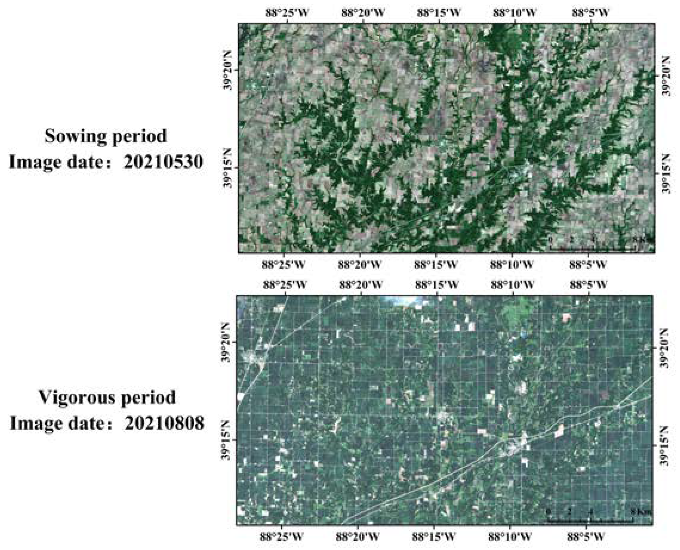
The geographical location of the study area is shown in Figure 1. The study area was located in the eastern part of Hulunbuir City, including the four regions of Molidawa Daur Autonomous Banner, Oroqen Autonomous Banner, Arong Banner and Zalantun City. The eastern part of the study area was bordered by the Nenjiang River and Heilongjiang Province, while the western part was bordered by the Daxinganling Mountains. The study area had an altitude of 200–500 m, an annual precipitation rate of 500–800 mm, fertile soil and high natural fertility, forming an agricultural economic zone that is mainly used for planting, with soybean and corn being the main crop types. The geographical location of the study area is shown in Figure 1.
We surveyed plot crop types at 2292 coordinate points in the study area, but did not include plot boundary information, and we sampled within and at the boundaries of these plots, using the sampled pixel points to produce training samples. In total, we sampled 90,000 soybean pixels, 130,000 corn pixels, and 320,000 pixels of other background samples. The training samples were centered on the sampled pixel points and we expanded their 5 × 5 neighborhood windows as training patches, where only the central pixel was labeled and the other pixels within the window were unlabeled and used to provide spatial information and more spectral information to the central target pixel. The validation data were based on the surveyed plot types as well as manual visual interpretations, combined with the full pixel labels manually outlined by the images, which were used to validate the model’s accuracy. The distribution of the reference data sites is shown in Figure 2.

2.2. Image Dataset

Sentinel-2 is a high-resolution multispectral imaging satellite that is divided into two satellites (A and B), which can cover 13 spectral bands with spatial resolutions of 10, 20 and 60 m. The A and B satellites operate simultaneously, with revisit cycles of up to 5–8 days, and can take multiple images during each crop-growth stage. Among the optical data, Sentinel-2 satellite data are the only data that contain three bands in the red edge range, which are very effective for monitoring vegetation health and predicting food production rates [27]. Therefore, we used Sentinel-2’s atmospherically corrected level 2A product as the input image.
Due to the influence of weather, image quality and revisit interval, it was difficult to obtain images during all phenological stages of crop growth; therefore, the requirement for the temporal resolution of images needed to be reduced. In this study, the notion of change detection was utilized in the selection of the time-series data to enhance the differentiation between crops and between crops and other vegetation using the two most different phenological periods: the sowing and vigorous periods. According to the analysis of soybean and corn phenology conducted in the study area, they have similar phenological periods [42]. During the sowing period, the soybean and corn had just been sown and there were no obvious features on the remote sensing images; therefore, the target farmland was bare ground. During this time window, the cultivated land used for the target crops clearly contrasted with the other non-target vegetation, such as woodland and grassland. During the vigorous period, NDVI reached its peak, crop leaf area reached its maximum and photosynthesis was strong. The crop characteristics were obvious in the remote sensing images and the differences between the different crops were clear; therefore, this was the most favorable period to distinguish different crops. Therefore, after analyzing the crop phenology within the study area, the two key time windows that presented the greatest differences in characteristics and the most obvious and stable characteristics were the sowing and vigorous periods [42,43]. The images obtained from these time windows within the study area were used as inputs to build our model, as shown in Figure 2.

3. Methodology

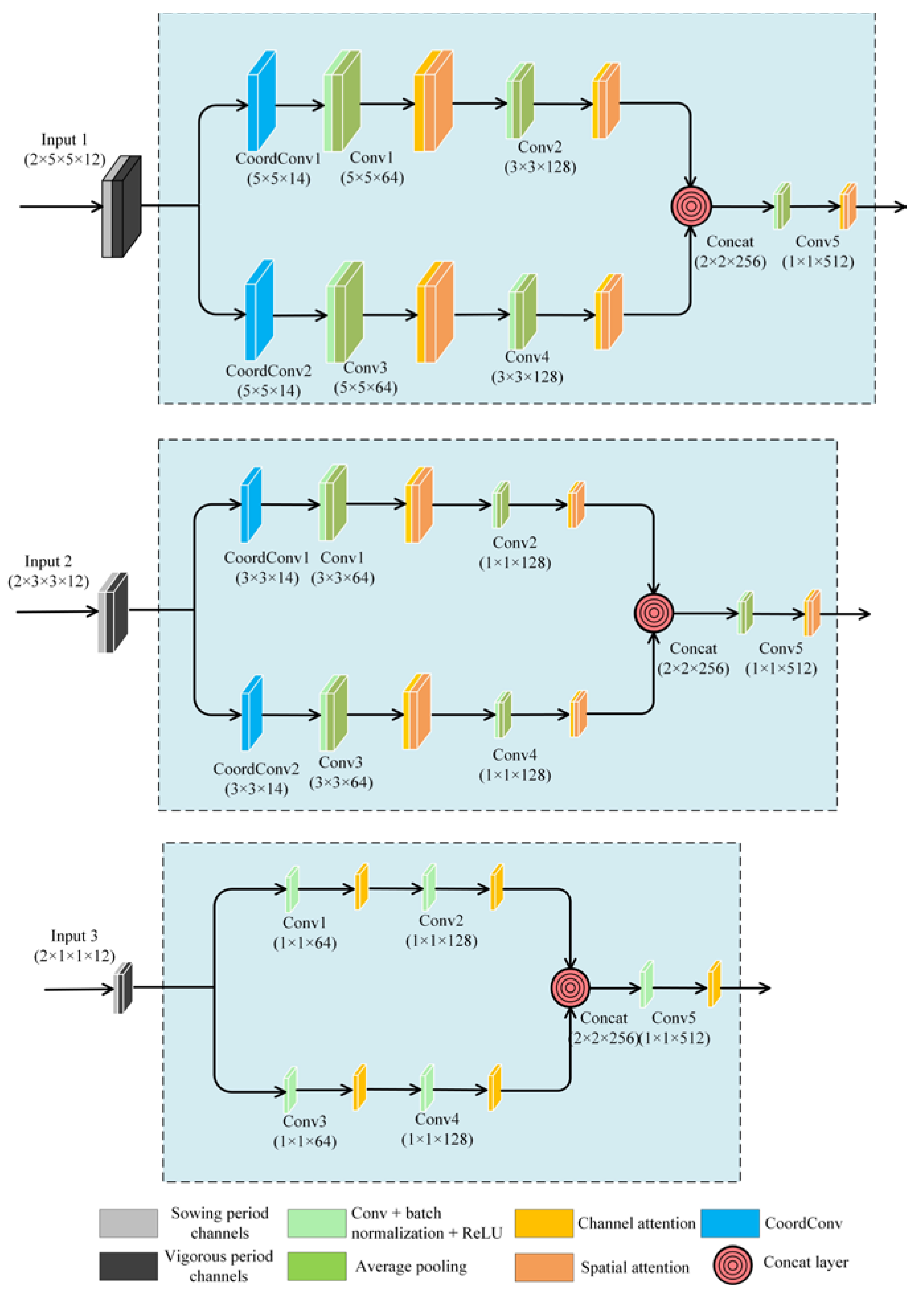
3.1. Network Structure

When pixel-level samples are used as inputs for convolutional networks, one-dimensional convolution often only learns the spectral information of a single pixel in isolation. However, without considering the spatial correlations between neighboring pixels, the generated crop thematic maps may present a considerable amount of salt and pepper noise. In addition, mixed pixels on different plot boundaries may cause the edges between them to appear unclear. To address these problems, we used a pixel sample with annotations as the central pixel, extended its surrounding 5 × 5 neighborhood window to be used as the model input and designed a multiscale attentional convolutional network (MACN). The spatial and spectral features at 1 × 1, 3 × 3 and 5 × 5 scales were extracted using multiscale network extraction. The network structure is shown in Figure 3.
Specifically, a dual-temporal 5 × 5 sample input was divided into three scales (1 × 1, 3 × 3 and 5 × 5) centered on the target pixel, and then multiple parallel-connected branching networks were used to learn the spatial and spectral features of different sizes and fuse them, as shown in Figure 4. For the mixed pixels at the edge of the plot, the consistency of the pixels within the neighborhood window dramatically changed. Therefore, we introduced coordinate convolution to the input layers of 3 × 3 and 5 × 5 branches to enhance the spatial relationship between the central and neighboring pixels to perceive the change in pixels occurring at the edge of the cultivated plots from crop to non-cultivated plots, so that the model could perceive the boundary information of cultivated plots and constrain the attention to the interior of the cultivated plots. In each branch network, mixed spatial and spectral information was extracted using a convolutional layer, followed by the CBAM, which processed the feature maps containing the mixed information. The CBAM was adjusted for the different network branches within the MACN. For the 3 × 3 and 5 × 5 branches, the channel attention module was used to enhance the interactions between spectral and temporal channels (sowing- and vigorous-period channels) and actively learn the spectral variation patterns under different temporal sequences. The vigorous- and sowing-period channels were convolved separately for the feature extraction of their respective periods and were fused after two layers of convolution. Then, co-convolution was performed to extract the phenological difference and crop features. Then, the spatial attention module was used to capture the contribution weights of the pixel information in the neighborhoods around the central pixel. For the 1 × 1 branch, only the channel attention module was used to capture the relationships between the different temporal channels. Finally, the multiscale features that were extracted from the different branches were combined. The fusion of the different-scale feature channels was completed by the convolutional attention module and the classification results for the target pixel were produced by a double-layer fully connected layer and a Softmax classifier.

3.2. Coordinate Convolution

In practical crop mapping, the accuracy of crop-plot boundaries is of great significance for crop-yield estimations and agricultural-refinement management. Due to the resolution, plot boundaries have a high number of mixed pixels and the traditional pixel-based crop-classification methods cannot use spatial information effectively to determine plot boundaries. In this study, we used a 5 × 5 neighborhood window to provide spatial information for target pixels to solve the problem of missing spatial information in other pixel-based methods. In addition, ordinary convolution cannot effectively extract spatial-feature location information because the lack of coordinate information for input features leads to the loss of a large amount of spatial-location information, especially boundary- and fine-feature information, at multiple scales by successive convolutional operations. Therefore, Liu et al. [39] proposed a coordinate transformation module to solve the problem of difficult coordinate transformation by ordinary convolution. By using an additional coordinate channel, coordinate convolution can obtain the input coordinates of a target during the convolution process and extract the spatial-location information from the target features as an additional channel to be stitched with the original features. Specifically, the construction of CoordConv that was used in this study is shown in Figure 5. With the help of the coordinate convolution module, more spatial-information features could be used in the next convolution step, thus increasing the detail and reducing information loss.

3.3. Convolutional Block Attention Module

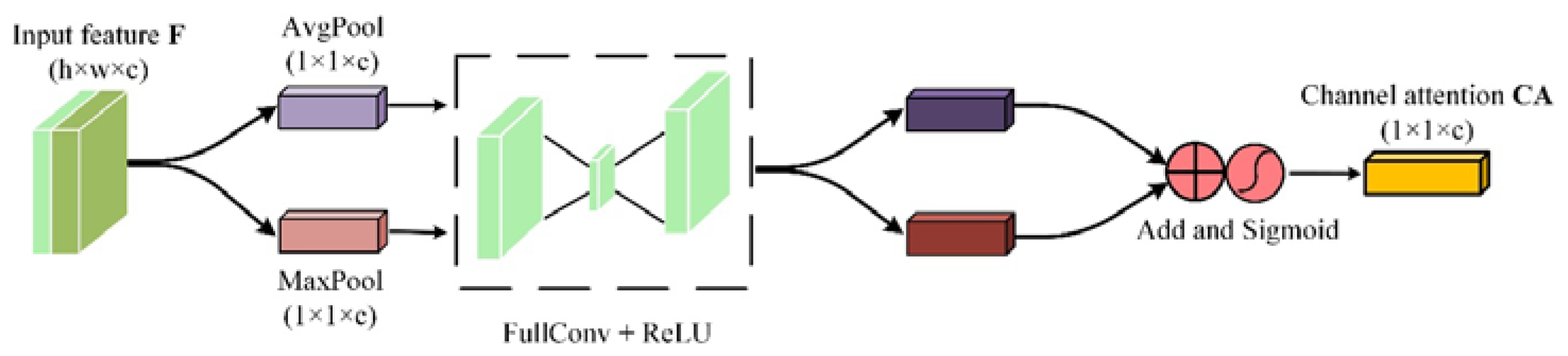
3.3.1. Channel Convolutional Attention Module

The channel convolutional attention module was based on the channel attention module. Unlike the original channel attention module, the channel convolutional attention module replaced the two-layer MLP with two layers of full convolution. Full convolution was used to better fuse channel information and improve the interactions between different feature channels to improve the performance of deep neural networks. Specifically, our module consisted of two pooling layers, two layers of full convolution and an activation function. The process is shown in Figure 6. In this module, the input feature maps (h × w × c) were first squeezed by global and maximum pooling methods to obtain two (1 × 1 × c) vectors. Then, they were separately fed into the first layer of full convolution, and the size of the convolutional kernels was determined by the adaptive function, which was activated by the ReLu function following the convolution. Subsequently, they were fed into the second layer of full convolution. The squeezed and activated feature channels were reduced to (1 × 1 × c) to obtain two new (1 × 1 × c) feature vectors. Finally, the two obtained feature vectors were element-wise added and activated by the sigmoid function to obtain the final channel attention (CA) weights. The channel convolutional attention weights are calculated as
C A = σ ( F C ( A v g P o o l ( F ) ) + F C ( M a x P o o l ( F ) ) )
where σ is the sigmoid activation function, F is the input feature map and FC represents the fully convolutional network.

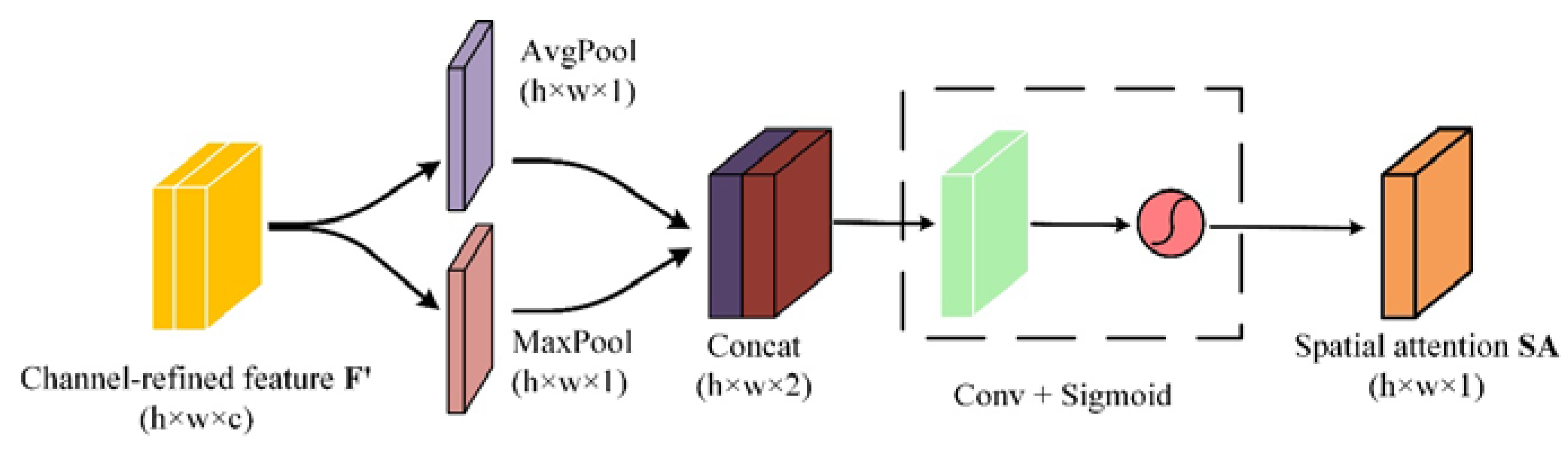
3.3.2. Spatial Convolutional Attention Module

The spatial convolutional attention module (SAM) consists of two pooling layers, a convolutional layer and a sigmoid activation function. The spatial feature information was used to capture the correlations between different local regions within the input image, and spatial attention maps were generated by learning the importance of different spatial locations within the neighborhood. The specific process is shown in Figure 7. Firstly, the input feature map was pooled at the mean and maximum values of the channel dimensions, then the squeezed spatial feature maps were merged and the merged feature maps were fused using a step size of 1 and a convolutional kernel size of 1 × 1. Finally, the spatial attention (SA) weights were obtained by activating the sigmoid function. The spatial convolutional attention weights are computed as
S A = σ ( C o n v 1 × 1 ( A v g P o o l ( F ) ; M a x P o o l ( F ) )
where σ is the sigmoid activation function, F is the channel-refined feature, and C o n v 1 × 1 represents the 1 × 1 convolutional network.

3.3.3. Multiscale Convolutional Block Attention Module

Our CBAM was an attention mechanism module that combined the channel and spatial attention modules in two dimensions. These two modules performed adaptive feature selection and the enhancement of the input feature maps in the channel and spatial directions, respectively, thereby highlighting the main features and suppressing irrelevant features. In the CBAM, as shown in Figure 8, the feature map 𝐹 that was outputted from the previous layer of convolution was converted into a one-dimensional channel attention (CA) map using the channel attention module. Then, the input feature map 𝐹 was element-wise multiplied by the CA map to obtain the salient feature map F in the channel direction. The spatial attention module then converted F’ into a two-dimensional spatial attention (SA) map. Finally, F was element-wise multiplied by the SA map to obtain the output feature map F , which is calculated as
F = C A × F
F = S A × F
In this study, multiscale convolution combined with CBAM was used to construct a multiscale attentional convolutional network structure. The CBAM was embedded for different convolutional scales, as well as different temporal channels, thus making the network pay more attention to the spectral and spatiotemporal information of target pixels to improve the accuracy of the crop mapping.

3.4. Implementation Details

In order to verify the effectiveness of the method in this paper, RFC [44], MLP [45] and Resnet [46] were selected as comparison models in this paper.
RFC: RFC is a supervised learning algorithm that uses an integrated learning algorithm with decision trees as the base learner and has the advantages of easy implementation and low computational overheads. Therefore, it is commonly used in simple crop-classification tasks or land-cover/land-use (LCLU) tasks [47].
MLP: MLP is the most classical artificial neural network (ANN), which contains input, hidden and output layers. The non-linear activation of the hidden layer by the activation function allows the neural network to learn from complex non-linear datasets. Recent studies have shown that MLP-based image-classification methods can achieve an image-classification performance comparable to CNN and a transformer without a convolution module and attention mechanism [48].
Resnet-18: Resnet is a classical CNN network. Resnet proposes the use of BN (batch normalization) layers to solve the problem of gradient disappearance or gradient explosion in CNNs. Resnet proposes a residual structure that artificially allows some layers of the neural network to skip the connection of the next layer of neurons to the deep network to alleviate the degradation problem. Resnet-18 is a network with seventeen convolutional layers and one fully connected layer.
The proposed model used TensorFlow 2.4 as the deep-learning framework and the development language was Python. This paper used an Adam optimizer to optimize the network and update the parameters with the initial learning rate set to 0.001. To better train the model, the learning rate was automatically adjusted as the training period increased to accelerate the convergence of the network combined with the optimization. This study used a multiclass cross-entropy loss function as the loss function. A total of 100 epochs were used in the training process and batch size was 2048. Additionally, to ensure a fair comparison of the different deep-learning methods, all compared deep-learning models presented the same learning rate, epoch and batch-size settings. The number of parameters of the MACN obtained from training was about 16.8M; the number of parameters of Resnet-18 was approximately 11.7M. The RFC used grid search and cross-validation methods for tuning, and the final RFC parameters were set as n estimators of 60, with max. features of 6 and max. depth of 13.

3.5. Pixel-Level Accuracy Evaluation Metrics
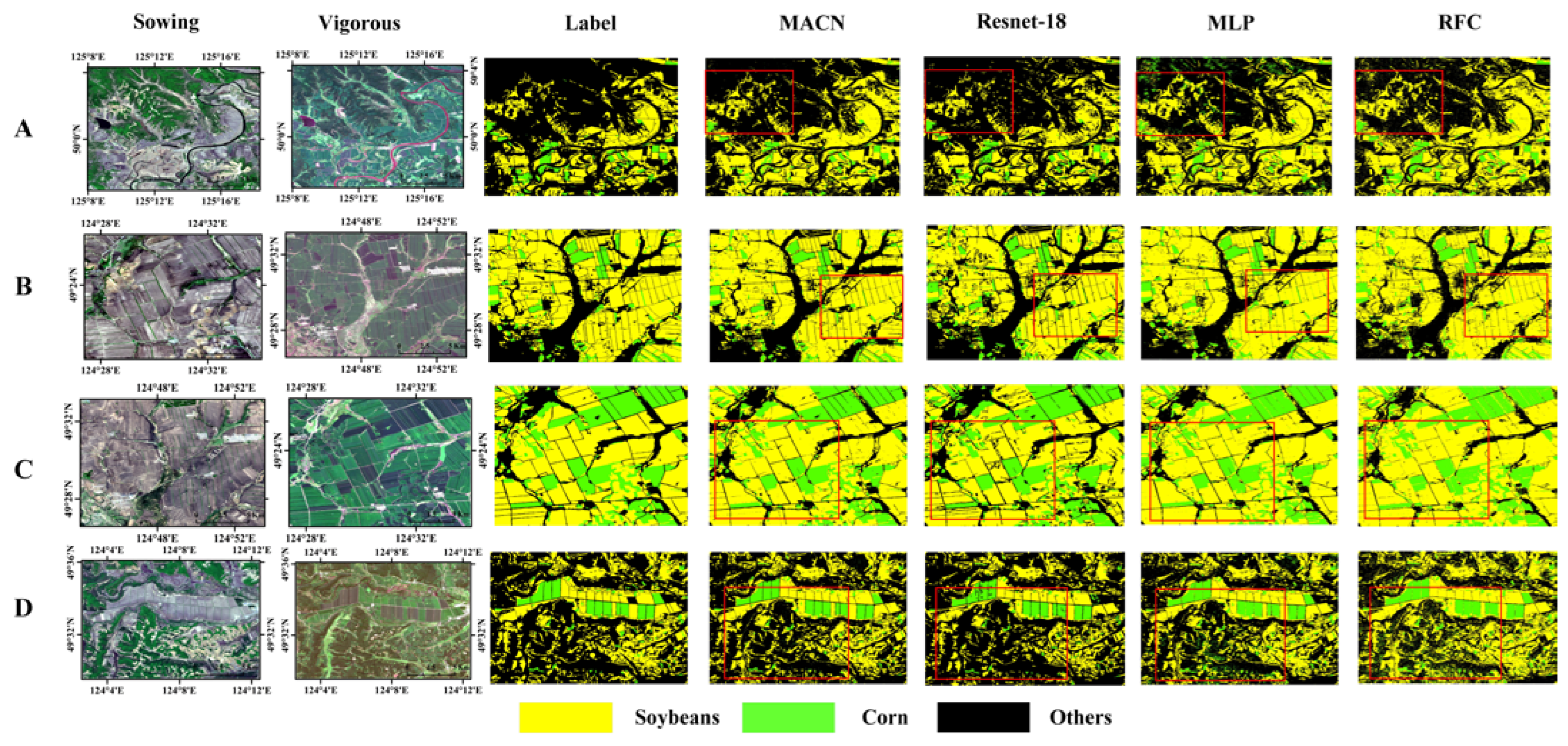
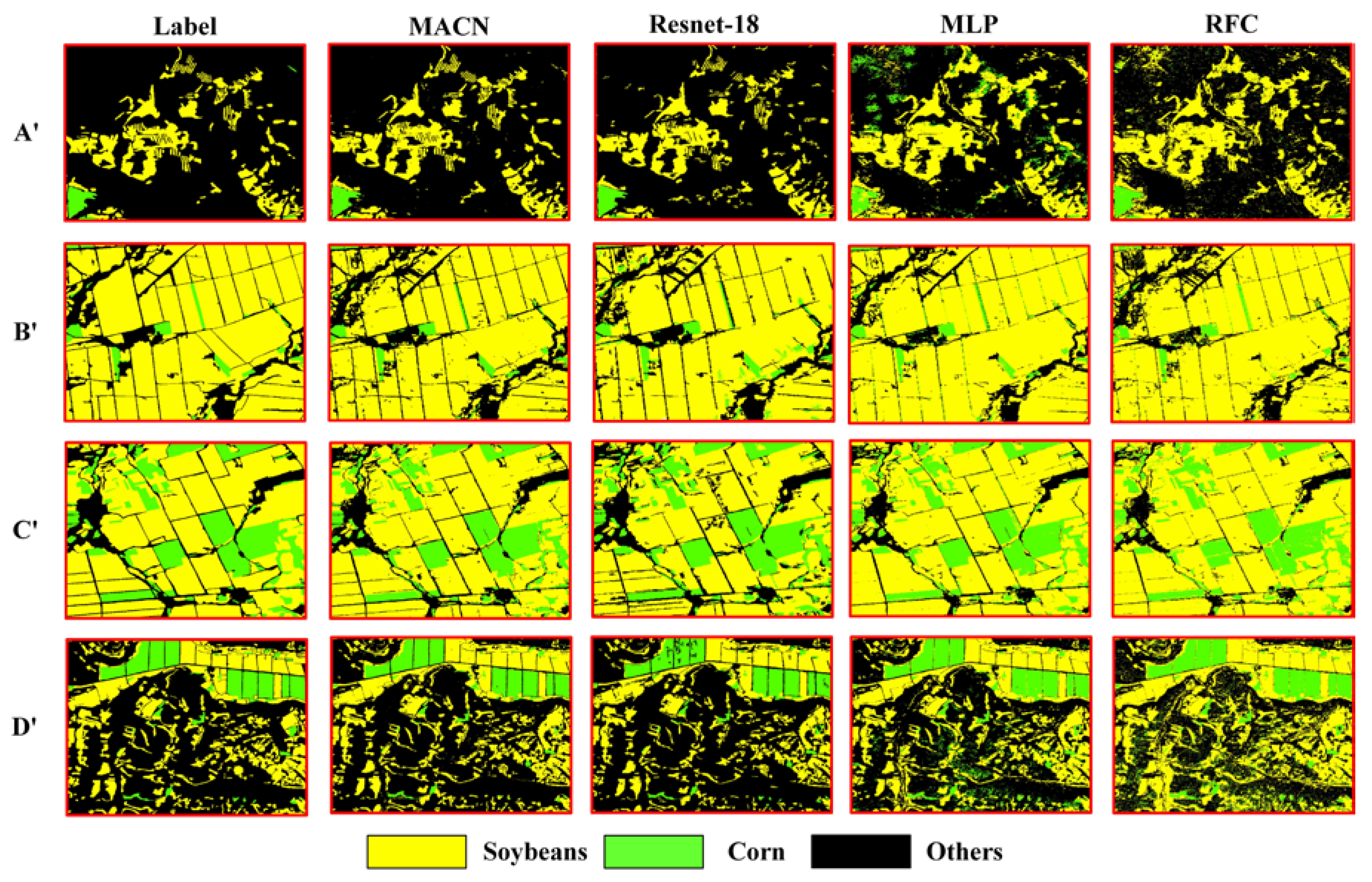
In this study, the accuracy of the crop-mapping results was evaluated using the overall accuracy (OA), the kappa coefficient, the F1 score and the intersection-over-union (IOU) ratio. OA refers to the ratio of the sum of the number of pixels in correctly identified categories to the total number of pixels in all of the identified categories within the test image. The kappa coefficient is a metric that is used for consistency testing, which can also be used to measure the effectiveness of classification practices. For classification problems, the so-called consistency refers to whether the model prediction results and actual classification results are consistent. Precision refers to the proportion of correct pixels in the prediction results and recall indicates the proportion of correct pixels in the ground truth results. The Recall [49], Precision [49], OA [49], F1 [50] score, IOU [51] and kappa [52] formulae are as follows:
O A = T P + T N N
P r e c i s i o n = T P T P + F P
R e c a l l = T P T P + F N
F 1 = 2 × P r e c i s i o n × R e c a l l P r e c i s i o n + R e c a l l
I O U = T P T P + F N + F P
P o = i = 1 C T i N
P e = i = 1 C ( a i × b i ) N × N
K a p p a = P o P e 1 P e
where TP represents true positive, FP represents false positive, TN represents true negative and FN represents false negative. N is the total number of samples and C is the total number of categories; then, the numbers of real samples in each category are a1, a2,..., aC and the predicted numbers of samples in each category are b1, b2,..., bC.

4. Results

The constructed model was tested on four areas that were not involved in its training, and the classification results were compared to those obtained from deep-learning and machine-learning models that are commonly used in crop-classification practices: Resnet-18, MLP and RFC. All the models were trained using the same training data and the input images and features were kept consistent. The accuracy evaluation of all experiments was based on all study areas, and the figures are shown as examples.
The overall extraction results from each model are shown in Figure 9. From the figure, it can be observed that among the four extraction methods, the overall extraction results obtained from the proposed method are the closest to the visual interpretation results, and the extraction results for the Resnet-18 and MLP are slightly worse than those of the proposed method. A qualitative analysis of the recognition results showed that all models performed well in the judgment of plot type and produced fewer misclassified and omitted plots, indicating that the two crop types could be effectively distinguished during the two phenological periods with the most significant differences in features. The red boxes in Figure 9 show the differences in the details between the results for the proposed method and other methods. Enlarged views of the red boxes are shown in Figure 10. In the enlarged views (Figure 10A’,D’) (which represent A and D in Figure 9), it can be observed that the MACN classification results present the least noise in the images out of the four algorithms and the plot shape is in high agreement with the real label. The RFC extraction results are the worst and there is a lot of noise in the images, indicating that the feature-extraction ability of RFC is slightly poorer than that of the other networks. The enlarged views (Figure 10B’,C’) (which represent B and C in Figure 9) show that it is difficult to consider low- and high-level spatial features comprehensively because of the model’s inability to consider spatial information and perceptual fields; therefore, the pixel-based Resnet-18, MLP and RFC models could not effectively distinguish between the mixed-image elements in plot-boundary ridges, and the plot boundaries were fuzzy. In contrast, the MACN could effectively distinguish between the ridges between plots and the plots themselves based on neighborhood windows, and the extracted plot boundaries were clearer.
To quantitatively validate the performance of the proposed method, the accuracy scores for the MACN were compared for the different types of crops in each test area (Table 1). As a whole, the OA scores of the extraction results for the four test areas are 0.9321, 0.9598, 0.9435 and 0.9569. The average OA, kappa coefficient, F1 score and IOU of the extraction results for the four test areas are 0.9481, 0.9115, 0.9307 and 0.8729, respectively. Specifically for each category, the extraction results for soybean and corn reached 0.9327 and 0.9286 in terms of the F1 score and 0.8761 and 0.8697 in terms of IOU, respectively.
Table 2 shows the average accuracy scores of the proposed method and the compared crop extraction methods (Resnet-18, MLP and FRC) for the four test areas. As can be observed in Table 2, compared to the more classical Resnet-18 network model for image-classification purposes, the proposed model presents nearly 3%, 6% and 4% improvements in the OA, kappa coefficient and F1 score, respectively. Compared to MLP, which has performed well in remote sensing time-series crop-classification tasks in recent years, the proposed model presents 13%, 24% and 5% improvements, respectively. In contrast, the average OA and kappa coefficients of the RFC method for the four measurement areas are 0.7846 and 0.6496, which demonstrate the worst performance among the four extraction methods. From the network perspective, the RFC network, which is suitable for performing simple feature extractions, was ineffective in learning the spatiotemporal variations in crop features after fusing the two image bands. In addition, the pixel-based Resnet-18 and MLP models could not take into account the spatial information of the target pixels; therefore, the proposed method scored 7–9% higher than the Resnet-18 and MLP methods in terms of IOU when evaluating the shape of the extraction results. In general, the proposed method outperformed the other deep-learning methods for crop-classification extraction, both in terms of type judgment and shape extraction.

5. Discussion

The results presented above show that our method significantly reduces the noise of the classification results by opening windows and introducing coordinate convolution and CBAM mechanisms, and the shape and boundaries of the plots are guaranteed.

5.1. Validity of Window Size

Figure 11 shows the multisize networks with different window sizes. It can be observed from the figure that the network that was based on the 1 × 1 window, which was based on the extraction results obtained from the pixels themselves, presents a considerable amount of noise and blurred boundaries. As the window size increases, the noise gradually decreases, the boundaries gradually become clearer and the accuracy scores gradually increase. When the window size is 5 × 5, the level of noise in the images is already very low, but when the window size continues to increase to 7 × 7 or 9 × 9, the mapping results no longer significantly improve.
The average accuracy scores of the networks at different scales for the four test areas are presented in Table 3. In terms of accuracy, the 1 × 1 window network also had the lowest accuracy evaluation metrics among all of the models. The OA and kappa coefficients were 0.9481 and 0.9115, respectively, when the window size was 5 × 5, which were the highest scores among the five scales. Moreover, as the window size and number of network branches increased, the parameters of the network also upgraded. Therefore, we observed that the 5 × 5 window was more suitable for crop-mapping tasks, and that it cannot only reduce the noise in the classification results, but also accurately extract the shape and boundary of the plot.
In addition to the discussion of the window size, we also discussed the effect of different branches of the MACN network. Figure 11 visualized the feature maps of three branches in the MACN, namely, MACN_1 × 1, MACN_3 × 3 and MACN_5 × 5 branches. From Figure 12, it can be observed that the different branches of interest are partially complementary. The 1 × 1 branch focuses on the furrow and tree row. The MACN_3 × 3 branch has a greater focus on soybean and a relatively lower focus on corn. The MACN_5 × 5 branch, on the other hand, is more concerned with corn and relatively less concerned with soybean. The feature map of the MACN with three scale branches is comprehensive and correct. The network focused its attention on the soybean and corn plots, and it showed less interest in the field ridges and furrows.
We performed branch reductions for the MACN with three branches. The role of different branches in the network was observed by continuously clipping the low-semantic branches. As can be observed from the extraction results (Figure 13), the classification results of the network that clipped out the 1 × 1 branch and contained 3 × 3 + 5 × 5 show some noise due to under-classification. The classification results of the network that clipped out the 1 × 1 and 3 × 3 branches and included only the 5 × 5 window show some missed scores of soybean plots, which may be related to the lack of 3 × 3 branch focus on soybean plots. The MACN with three scale branches can comprehensively take into account the features of different sizes and obtain multiscale feature information through different-sized perceptual fields, which effectively alleviates the phenomenon of crop omission and misclassification.
We present the accuracy of the ablation experiments in Table 4. In the quantitative accuracy evaluation, the network containing only a single 5 × 5 window branch has an overall accuracy (OA) of 0.9294 and a kappa coefficient of 0.8671, which is approximately 1.9% and 4.4% lower compared to the MACN, respectively, and an F1 score of 0.9054 for soybean, which is approximately 3% lower compared to the MACN. The MACN with three branches presents the highest performance value in each accuracy evaluation index. The OA and kappa coefficients gradually decrease as the number of branches decreases. This indicates that the MACN effectively combines the features of different scale branches by multiplexing and enhancing the multiscale features.

5.2. The Role of CBAM and Coordinate Convolution in MACN Networks

Furthermore, we explored the roles of coordinate convolution and the attention mechanisms in the network. We ablated the coordinate convolution by removing the coordinate channels of the input layer on top of the MACN. The attention mechanism was ablated by removing the CBAM module following each convolutional layer in the MACN. We named the experimental results as Missing CoordConv and Missing CBAM, respectively.
The feature maps of different models are shown in Figure 14, from which it can be observed that the different models are basically correct in judging the plots of crops grown. The network with a missing coordinate convolution is ambiguous in its interest in the boundary, and in the MACN network that includes coordinate convolution it can be observed that the feature maps obtained are relatively good in judging the shape of the plots, indicating that the coordinate convolution effectively constrains the model’s attention to the target plots. From the classification results (Figure 15), it can be observed that the network has a missing coordinate convolution, the judgment of plot boundaries is ambiguous, the plots are connected to each other, and many fine-field gullies are incorrectly classified as crops, while the MACN with a coordinate convolution included has clear boundaries between planted and non-planted plots in the classification results. For the network with Missing CBAM, the feature maps obtained presented low sensitivity to the target plots as a whole, and there was a considerable amount of noise and gaps inside the plots in the corresponding extraction results. For the MACN model incorporating the attention mechanism, the obtained feature maps presented high sensitivity to the cultivated land and low sensitivity to the non-cultivated land, with fewer voids and noises in the classification results.
As shown in Table 5, the MACN showed good results in terms of the OA and kappa coefficient. This indicated that CoordConv and CBAM were effective in extracting the crop features. The average IOU of MACN was 0.8729, which was higher than that of the Missing CoordConv with IOU = 0.8358, indicating that CoordConv effectively enhances the location information of map-edge pixels and strengthens the features of mixed pixels at the edge of the map, making the contours of cultivated land clear. However, the OA and kappa values of the Missing CoordConv network were lower than those of Missing CBAM. This may be due to the fact that the spatial up–down information of the target pixels was enhanced by the coordinate convolution, but not well utilized. The MACN performs well in various accuracy evaluation metrics, showing high accuracy values. This result suggests that both CBAM and coordinate convolution modules are essential for our network. The MACN could effectively utilize the attention mechanisms and coordinate convolution to improve classification and mapping accuracy.

5.3. Spatial Generalizability

Without adding samples, we tested the soybean–corn distribution in Cumberland County. Cumberland County is a county located in the US state of Illinois, located at 88°00′-88°28′W, 39°10′-39°22′N. We verified the accuracy using the cropland data layer (CDL), with data published by the USDA. Figure 16 shows the mapping results of the soybean–corn distribution and MACN in CDL data; from Figure 16, we can observe that our mapping results are similar to the CDL data and the consistency of judgment for plot type is high. Based on the CDL data, we calculated the classification accuracy of the MACN. The results of the accuracy evaluation are presented in Table 6. Relative to the CDL data, the overall accuracy (OA) of the MACN is 0.8466, the kappa coefficient is 0.7646, the mean F1 score for soybean–corn is 0.8483 and the mean IOU is 0.7367. This shows that our proposed network is not only energy efficient in extracting crop features using multiscale windows, but also ensures the spatial generalization of the method.

6. Conclusions

In order to overcome the problem that noise and unclear boundaries in the crop mapping of pixel-based classification methods caused by crop spectral similarity and mixed pixels, we designed a multiscale attentional convolutional network. In this network, the multiscale convolution was used to obtain the spatial–spectral features in target pixel domains and reduce the pretzel noise phenomenon and boundary-ambiguity problems of pixel-based crop-mapping methods, the coordinate convolution was used to enhance the spatial features of a target pixel field and a CBAM was used to enhance the spectral and temporal features of a target pixel field. The comparison experiment showed that our method significantly improved the noise and unclear boundaries in pixel-based crop mapping compared with other methods. In addition, the comparison of the experimental results obtained from different neighborhood window sizes shows that the noise and boundary blurring that occurs in crop mapping could be effectively reduced by extending the neighborhood windows. The ablation experiments showed that the coordinate convolution can effectively enhance the location information of the graph-edge pixels and enhance the features of the edge-blend pixels of the graph to create clear contours of the cultivated land; the attention mechanism also plays an active role in the network by enhancing the spectral and phenological features of the crops, reducing the noise that appears in the classification results. The generalization validation in 2021 in Cumberland, USA, shows that the method not only improves the accuracy, but also has spatial generalization. Therefore, the method proposed in this study could provide reliable technical support for remotely sensed crop mapping. Although the method in this paper improved the noise and boundaries in multitemporal remotely sensed crop mapping, there are still numerous challenges (plot size, low spatial resolution) for remotely sensed crop-mapping practices. In future research, we will focus on these influencing factors and attempt to obtain solutions.

Author Contributions

Conceptualization, Y.W. and H.Y.; methodology, Y.W.; validation, Y.W.; investigation, Y.W. and B.W.; resources, Y.W. and Y.W.; data curation, B.W.; writing—original draft preparation, Y.W.; writing—review and editing, Y.W. and H.Y.; funding acquisition, Y.W., H.Y. and B.W. All authors have read and agreed to the published version of the manuscript.

Funding

This research was funded by the National Natural Science Foundation of China (grant No. 42101381, 41901282 and 41971311), the National Natural Science Foundation of Anhui (grant No. 2008085QD188), the Science and Technology Major Project of Anhui Province (grant No. 201903a07020014) and the Anhui Provincial Key R&D International Cooperation Program (grant No. 202104b11020022).

Institutional Review Board Statement

“Not applicable” for studies not involving humans or animals.

Informed Consent Statement

“Not applicable” for studies not involving humans.

Data Availability Statement

The data presented in this study are available on request from the corresponding author. The data are not publicly available due to the permissions issues.

Conflicts of Interest

The authors declare no conflict of interest.

References

  1. Godfray, H.C.J.; Beddington, J.R.; Crute, I.R.; Haddad, L.; Lawrence, D.; Muir, J.F.; Pretty, J.; Robinson, S.; Thomas, S.M.; Toulmin, C. Food Security: The Challenge of Feeding 9 Billion People. Science (1979) 2010, 327, 812–818. [Google Scholar] [CrossRef] [PubMed] [Green Version]
  2. Foley, J.A.; Ramankutty, N.; Brauman, K.A.; Cassidy, E.S.; Gerber, J.S.; Johnston, M.; Mueller, N.D.; O’Connell, C.; Ray, D.K.; West, P.C.; et al. Solutions for a Cultivated Planet. Nature 2011, 478, 337–342. [Google Scholar] [CrossRef] [PubMed] [Green Version]
  3. Food Security, Farming, and Climate Change to 2050: Scenarios, Results, Policy Options; International Food Policy Research Institute: Washington, DC, USA, 2010.
  4. Rogan, J.; Franklin, J.; Roberts, D.A. A Comparison of Methods for Monitoring Multitemporal Vegetation Change Using Thematic Mapper Imagery. Remote Sens. Environ. 2002, 80, 143–156. [Google Scholar] [CrossRef]
  5. Scott, G.; Rajabifard, A. Sustainable Development and Geospatial Information: A Strategic Framework for Integrating a Global Policy Agenda into National Geospatial Capabilities. Geo-Spat. Inf. Sci. 2017, 20, 59–76. [Google Scholar] [CrossRef] [Green Version]
  6. Benz, U.C.; Hofmann, P.; Willhauck, G.; Lingenfelder, I.; Heynen, M. Multi-Resolution, Object-Oriented Fuzzy Analysis of Remote Sensing Data for GIS-Ready Information. ISPRS J. Photogramm. Remote Sens. 2004, 58, 239–258. [Google Scholar] [CrossRef]
  7. Luo, C.; Qi, B.; Liu, H.; Guo, D.; Lu, L.; Fu, Q.; Shao, Y. Using Time Series Sentinel-1 Images for Object-Oriented Crop Classification in Google Earth Engine. Remote Sens. 2021, 13, 561. [Google Scholar] [CrossRef]
  8. Garcia-Pedrero, A.; Lillo-Saavedra, M.; Rodriguez-Esparragon, D.; Gonzalo-Martin, C. Deep Learning for Automatic Outlining Agricultural Parcels: Exploiting the Land Parcel Identification System. IEEE Access 2019, 7, 158223–158236. [Google Scholar] [CrossRef]
  9. Jiao, X.; Kovacs, J.M.; Shang, J.; McNairn, H.; Walters, D.; Ma, B.; Geng, X. Object-Oriented Crop Mapping and Monitoring Using Multi-Temporal Polarimetric RADARSAT-2 Data. ISPRS J. Photogramm. Remote Sens. 2014, 96, 38–46. [Google Scholar] [CrossRef]
  10. Geirhos, R.; Michaelis, C.; Wichmann, F.A.; Rubisch, P.; Bethge, M.; Brendel, W. Imagenet-Trained CNNs Are Biased towards Texture; Increasing Shape Bias Improves Accuracy and Robustness. In Proceedings of the 7th International Conference on Learning Representations, ICLR 2019, New Orleans, LA, USA, 6–9 May 2019. [Google Scholar]
  11. sainte Fare Garnot, V.; Landrieu, L.; Giordano, S.; Chehata, N. Satellite Image Time Series Classification with Pixel-Set Encoders and Temporal Self-Attention. In Proceedings of the IEEE Computer Society Conference on Computer Vision and Pattern Recognition, Seattle, WA, USA, 13–19 June 2020. [Google Scholar]
  12. Alganci, U.; Sertel, E.; Ozdogan, M.; Ormeci, C. Parcel-Level Identification of Crop Types Using Different Classification Algorithms and Multi-Resolution Imagery in Southeastern Turkey. Photogramm. Eng. Remote Sens. 2013, 79, 1053–1065. [Google Scholar] [CrossRef]
  13. Garnot, V.S.F.; Landrieu, L. Panoptic Segmentation of Satellite Image Time Series with Convolutional Temporal Attention Networks. In Proceedings of the IEEE International Conference on Computer Vision, Montreal, QC, Canada, 10–17 October 2021. [Google Scholar]
  14. Boryan, C.; Yang, Z.; Mueller, R.; Craig, M. Monitoring US Agriculture: The US Department of Agriculture, National Agricultural Statistics Service, Cropland Data Layer Program. Geocarto Int. 2011, 26, 341–358. [Google Scholar] [CrossRef]
  15. Fisette, T.; Rollin, P.; Aly, Z.; Campbell, L.; Daneshfar, B.; Filyer, P.; Smith, A.; Davidson, A.; Shang, J.; Jarvis, I. AAFC Annual Crop Inventory. In 2013 Second International Conference on Agro-Geoinformatics (Agro-Geoinformatics); IEEE: New York, NY, USA, 2013; pp. 270–274. [Google Scholar]
  16. Matikainen, L.; Karila, K.; Litkey, P.; Ahokas, E.; Munck, A.; Karjalainen, M.; Hyyppä, J. The challenge of automated change detection: Developing a method for the updating of land parcels. ISPRS Ann. Photogramm. Remote Sens. Spatial Inf. Sci. 2012, I-4, 239–244. [Google Scholar] [CrossRef] [Green Version]
  17. Xu, L.; Ming, D.; Zhou, W.; Bao, H.; Chen, Y.; Ling, X. Farmland Extraction from High Spatial Resolution Remote Sensing Images Based on Stratified Scale Pre-Estimation. Remote Sens. 2019, 11, 108. [Google Scholar] [CrossRef] [Green Version]
  18. Strothmann, W.; Ruckelshausen, A.; Hertzberg, J.; Scholz, C.; Langsenkamp, F. Plant Classification with In-Field-Labeling for Crop/Weed Discrimination Using Spectral Features and 3D Surface Features from a Multi-Wavelength Laser Line Profile System. Comput. Electron. Agric. 2017, 134, 79–93. [Google Scholar] [CrossRef]
  19. Rufin, P.; Frantz, D.; Ernst, S.; Rabe, A.; Griffiths, P.; özdoğan, M.; Hostert, P. Mapping Cropping Practices on a National Scale Using Intra-Annual Landsat Time Series Binning. Remote Sens. 2019, 11, 232. [Google Scholar] [CrossRef] [Green Version]
  20. Mathur, A.; Foody, G.M. Crop Classification by Support Vector Machine with Intelligently Selected Training Data for an Operational Application. Int. J. Remote Sens. 2008, 29, 2227–2240. [Google Scholar] [CrossRef] [Green Version]
  21. Yang, C.; Everitt, J.H.; Murden, D. Evaluating High Resolution SPOT 5 Satellite Imagery for Crop Identification. Comput. Electron. Agric. 2011, 75, 347–354. [Google Scholar] [CrossRef]
  22. Hu, Q.; Wu, W.-b.; Song, Q.; Lu, M.; Chen, D.; Yu, Q.-y.; Tang, H.-j. How Do Temporal and Spectral Features Matter in Crop Classification in Heilongjiang Province, China? J. Integr. Agric. 2017, 16, 324–336. [Google Scholar] [CrossRef]
  23. Zhang, J.; Feng, L.; Yao, F. Improved Maize Cultivated Area Estimation over a Large Scale Combining MODIS-EVI Time Series Data and Crop Phenological Information. ISPRS J. Photogramm. Remote Sens. 2014, 94, 102–113. [Google Scholar] [CrossRef]
  24. Blickensdörfer, L.; Schwieder, M.; Pflugmacher, D.; Nendel, C.; Erasmi, S.; Hostert, P. Mapping of Crop Types and Crop Sequences with Combined Time Series of Sentinel-1, Sentinel-2 and Landsat 8 Data for Germany. Remote Sens. Environ. 2022, 269, 112831. [Google Scholar] [CrossRef]
  25. Preidl, S.; Lange, M.; Doktor, D. Introducing APiC for Regionalised Land Cover Mapping on the National Scale Using Sentinel-2A Imagery. Remote Sens. Environ. 2020, 240, 111673. [Google Scholar] [CrossRef]
  26. Zhong, L.; Hu, L.; Zhou, H. Deep Learning Based Multi-Temporal Crop Classification. Remote Sens. Environ. 2019, 221, 430–443. [Google Scholar] [CrossRef]
  27. Vuolo, F.; Neuwirth, M.; Immitzer, M.; Atzberger, C.; Ng, W.T. How Much Does Multi-Temporal Sentinel-2 Data Improve Crop Type Classification? Int. J. Appl. Earth Obs. Geoinf. 2018, 72, 122–130. [Google Scholar] [CrossRef]
  28. Ji, S.; Zhang, Z.; Zhang, C.; Wei, S.; Lu, M.; Duan, Y. Learning Discriminative Spatiotemporal Features for Precise Crop Classification from Multi-Temporal Satellite Images. Int. J. Remote Sens. 2020, 41, 3162–3174. [Google Scholar] [CrossRef]
  29. Yuan, Q.; Shen, H.; Li, T.; Li, Z.; Li, S.; Jiang, Y.; Xu, H.; Tan, W.; Yang, Q.; Wang, J.; et al. Deep Learning in Environmental Remote Sensing: Achievements and Challenges. Remote Sens. Environ. 2020, 241, 111716. [Google Scholar] [CrossRef]
  30. Luo, C.; Meng, S.; Hu, X.; Wang, X.; Zhong, Y. Cropnet: Deep Spatial-Temporal-Spectral Feature Learning Network for Crop Classification from Time-Series Multi-Spectral Images. In Proceedings of the International Geoscience and Remote Sensing Symposium (IGARSS), Virtual, 26 September–2 October 2020. [Google Scholar]
  31. Xu, J.; Zhu, Y.; Zhong, R.; Lin, Z.; Xu, J.; Jiang, H.; Huang, J.; Li, H.; Lin, T. DeepCropMapping: A Multi-Temporal Deep Learning Approach with Improved Spatial Generalizability for Dynamic Corn and Soybean Mapping. Remote Sens. Environ. 2020, 247, 111946. [Google Scholar] [CrossRef]
  32. Chamorro Martinez, J.A.; Cué La Rosa, L.E.; Feitosa, R.Q.; Sanches, I.D.A.; Happ, P.N. Fully Convolutional Recurrent Networks for Multidate Crop Recognition from Multitemporal Image Sequences. ISPRS J. Photogramm. Remote Sens. 2021, 171, 188–201. [Google Scholar] [CrossRef]
  33. Vaswani, A.; Shazeer, N.; Parmar, N.; Uszkoreit, J.; Jones, L.; Gomez, A.N.; Kaiser, Ł.; Polosukhin, I. Attention Is All You Need. In Proceedings of the Advances in Neural Information Processing Systems, Long Beach, CA, USA, 4–9 December 2017; Volume 2017. [Google Scholar]
  34. Xu, J.; Yang, J.; Xiong, X.; Li, H.; Huang, J.; Ting, K.C.; Ying, Y.; Lin, T. Towards Interpreting Multi-Temporal Deep Learning Models in Crop Mapping. Remote Sens. Environ. 2021, 264, 112599. [Google Scholar] [CrossRef]
  35. Rußwurm, M.; Körner, M. Self-Attention for Raw Optical Satellite Time Series Classification. ISPRS J. Photogramm. Remote Sens. 2020, 169, 421–435. [Google Scholar] [CrossRef]
  36. Rußwurm, M.; Körner, M. Convolutional LSTMs for Cloud-Robust Segmentation of Remote Sensing Imagery. In Proceedings of the 32nd Conference on Neural Information Processing Systems, Montreal, QC, Canada, 3–8 December 2018; pp. 1–8. [Google Scholar]
  37. Rußwurm, M.; Körner, M. Multi-Temporal Land Cover Classification with Sequential Recurrent Encoders. ISPRS Int. J. Geoinf. 2018, 7, 129. [Google Scholar] [CrossRef] [Green Version]
  38. Ren, J.; Wang, R.; Liu, G.; Wang, Y.; Wu, W. An Svm-Based Nested Sliding Window Approach for Spectral–Spatial Classification of Hyperspectral Images. Remote Sens. 2021, 13, 114. [Google Scholar] [CrossRef]
  39. Liu, R.; Lehman, J.; Molino, P.; Such, F.P.; Frank, E.; Sergeev, A.; Yosinski, J. An Intriguing Failing of Convolutional Neural Networks and the CoordConv Solution. In Proceedings of the Advances in Neural Information Processing Systems, Montreal, QC, Canada, 3–8 December 2018; Volume 2018. [Google Scholar]
  40. Woo, S.; Park, J.; Lee, J.Y.; Kweon, I.S. CBAM: Convolutional Block Attention Module. In Proceedings of the Computer Vision–ECCV 2018, Munich, Germany, 8–14 September 2018; Volume 11211. [Google Scholar]
  41. Wang, Y.; Zhang, Z.; Feng, L.; Ma, Y.; Du, Q. A New Attention-Based CNN Approach for Crop Mapping Using Time Series Sentinel-2 Images. Comput. Electron. Agric. 2021, 184, 106090. [Google Scholar] [CrossRef]
  42. Zhong, L.; Gong, P.; Biging, G.S. Efficient Corn and Soybean Mapping with Temporal Extendability: A Multi-Year Experiment Using Landsat Imagery. Remote Sens. Environ. 2014, 140, 1–13. [Google Scholar] [CrossRef]
  43. Zhou, Y.; Xiao, X.; Qin, Y.; Dong, J.; Zhang, G.; Kou, W.; Jin, C.; Wang, J.; Li, X. Mapping Paddy Rice Planting Area in Rice-Wetland Coexistent Areas through Analysis of Landsat 8 OLI and MODIS Images. Int. J. Appl. Earth Obs. Geoinf. 2016, 46, 1–12. [Google Scholar] [CrossRef] [PubMed] [Green Version]
  44. Breiman, L. Random Forests. Mach. Learn. 2001, 45, 5–32. [Google Scholar] [CrossRef] [Green Version]
  45. Tu, Z.; Talebi, H.; Zhang, H.; Yang, F.; Milanfar, P.; Bovik, A.; Li, Y. MAXIM: Multi-Axis MLP for Image Processing. In Proceedings of the 2022 IEEE Conference on Computer Vision and Pattern Recognition (CVPR), New Orleans, LA, USA, 19–24 June 2022; pp. 5759–5770. [Google Scholar] [CrossRef]
  46. He, K.; Zhang, X.; Ren, S.; Sun, J. Deep Residual Learning for Image Recognition. In Proceedings of the 2016 IEEE Conference on Computer Vision and Pattern Recognition (CVPR), Las Vegas, NV, USA, 27–30 June 2016; Volume 2016, pp. 770–778. [Google Scholar] [CrossRef] [Green Version]
  47. Nguyen, L.H.; Joshi, D.R.; Clay, D.E.; Henebry, G.M. Characterizing Land Cover/Land Use from Multiple Years of Lansat and MODIS Time Series: A Novel Approach Using Land Surface Phenology Modeling and Random Forest Classifier. Remote Sens. Environ. 2020, 238, 111017. [Google Scholar] [CrossRef]
  48. Tolstikhin, I.; Houlsby, N.; Kolesnikov, A.; Beyer, L.; Zhai, X.; Unterthiner, T.; Yung, J.; Steiner, A.; Keysers, D.; Uszkoreit, J.; et al. MLP-Mixer: An All-MLP Architecture for Vision. Adv. Neural Inf. Process. Syst. 2021, 29, 24261–24272. [Google Scholar]
  49. Powers, D.M.W. Evaluation: From Precision, Recall and F-Factor to ROC, Informedness, Markedness & Correlation; School of Informatics and Engineering Flinders University: Adelaide, Australia, 2007. [Google Scholar]
  50. Sasaki, Y. The Truth of the F-Measure. Teach. Tutor. Mater. 2007, 1–5. Available online: https://www.researchgate.net/publication/268185911 (accessed on 1 September 2022).
  51. Rahman, M.A.; Wang, Y. Optimizing Intersection-Over-Union in Deep. In Proceedings of the International Symposium on Visual Computing, Las Vegas, NV, USA, 12–14 December 2016; pp. 234–244. [Google Scholar] [CrossRef]
  52. Cohen, J. A Coefficient of Agreement for Nominal Scales. Educ. Psychol. Meas. 1960, 20, 37–46. [Google Scholar] [CrossRef]
Figure 1. The geographical location of the study area.
Remotesensing 15 00047 g001
Figure 2. Distribution of reference data sites. Sowing period image data (left); vigorous period image data (right).
Remotesensing 15 00047 g002
Figure 3. The structure of our MACN.
Remotesensing 15 00047 g003
Figure 4. The different network branches within the MACN.
Remotesensing 15 00047 g004
Figure 5. The CoordConv added to two coordinate channels after the feature map was inputted: one for i and one for j coordinates (h and w represent the sizes of the feature map).
Remotesensing 15 00047 g005
Figure 6. The channel convolutional attention module.
Remotesensing 15 00047 g006
Figure 7. The spatial convolutional attention module.
Remotesensing 15 00047 g007
Figure 8. The convolutional block attention module.
Remotesensing 15 00047 g008
Figure 9. The recognition results for the different models in the four test areas.
Remotesensing 15 00047 g009
Figure 10. Enlarged views of the red boxes from the four test areas in Figure 9 (A’ corresponds to A, etc.).
Remotesensing 15 00047 g010
Figure 11. The classification results obtained from the different window sizes.
Remotesensing 15 00047 g011
Figure 12. The feature maps of the three branches of MACN.
Remotesensing 15 00047 g012
Figure 13. Classification results for different number of branches in the ablation experiment.
Remotesensing 15 00047 g013
Figure 14. The feature maps of MACN, Missing CoordConv and Missing CBAM.
Remotesensing 15 00047 g014
Figure 15. The classification results of MACN, Missing CoordConv and Missing CBAM.
Remotesensing 15 00047 g015
Figure 16. Soybean–corn distribution in Cumberland, Illinois, USA, in 2021 from CDL data and MACN.
Remotesensing 15 00047 g016aRemotesensing 15 00047 g016b
Table 1. The classification accuracy of crop classification, based on the MACN.
ImageSoybeanCornAverageAverageOAKappa
F1IOUF1IOUF1IOU
A0.8715 0.7722 0.8555 0.7475 0.8635 0.7599 0.9321 0.8772
B0.9666 0.9354 0.9653 0.9330 0.9660 0.9342 0.9598 0.9337
C0.9548 0.9134 0.9550 0.9140 0.9549 0.9137 0.9435 0.9101
D0.9380 0.8832 0.9386 0.8842 0.9383 0.8837 0.9569 0.9251
Average0.9327 0.8761 0.9286 0.8697 0.9307 0.8729 0.9481 0.9115
Table 2. The classification accuracy of crop classification using the different methods.
ModelSoybeanCornAverage F1Average IOUOAKappa
F1IOUF1IOU
MACN0.9327 0.8761 0.9286 0.8697 0.9307 0.8729 0.9481 0.9115
Resnet-180.8922 0.8068 0.8905 0.8040 0.8913 0.8054 0.9162 0.8523
MLP0.8863 0.8005 0.8688 0.7745 0.8775 0.7875 0.8139 0.6714
RFC0.8478 0.7415 0.8489 0.7423 0.8483 0.7419 0.7846 0.6496
Table 3. The crop-classification accuracy using the different window sizes.
Max. Window
Size
SoybeanCornAverage F1Average IOUOAKappa
F1IOUF1IOU
1 × 10.90170.82390.89430.81180.89800.81790.91370.8555
3 × 30.92520.86250.92090.8560.92310.85920.94220.9017
5 × 5 (MACN)0.93270.87610.92860.86970.93070.87290.94810.9115
7 × 70.910.83890.90850.83660.90930.83780.93040.8825
9 × 90.91690.8490.91260.84190.91480.84550.93430.8882
Table 4. Accuracy of crop classification for different numbers of branches.
ModelSoybeanCornAverage F1Average IOUOAKappa
F1IOUF1IOU
1 × 1 + 3 × 3 + 5 × 5 (MACN)0.9327 0.8761 0.9286 0.8697 0.9307 0.8729 0.9481 0.9115
3 × 3 + 5 × 50.9218 0.85540.91710.83060.91450.84300.94130.8722
5 × 50.90540.84120.89630.82550.90090.83340.92940.8671
Table 5. Accuracy of crop classification for MACN, Missing CoordConv and Missing CBAM.
ModelSoybeanCornAverage F1Average IOUOAKappa
F1IOUF1IOU
MACN0.9327 0.8761 0.9286 0.8697 0.9307 0.8729 0.9481 0.9115
Missing CoordConv0.8992 0.8620 0.90790.85850.90350.85860.90310.8532
Missing CBAM0.90330.82620.91610.84550.90970.83580.90850.8627
Table 6. Classification accuracy of MACN calculated from CDL data.
SoybeanCornAverageAverageOAKappa
F1IOUF1IOUF1IOU
0.8457 0.7327 0.8510 0.7406 0.84830.7367 0.8466 0.7646
Disclaimer/Publisher’s Note: The statements, opinions and data contained in all publications are solely those of the individual author(s) and contributor(s) and not of MDPI and/or the editor(s). MDPI and/or the editor(s) disclaim responsibility for any injury to people or property resulting from any ideas, methods, instructions or products referred to in the content.

