
Multi-Mission Satellite Detection and Tracking of October 2019 Sabiti Oil Spill in the Red Sea

 , , and
Abstract
:
1. Introduction
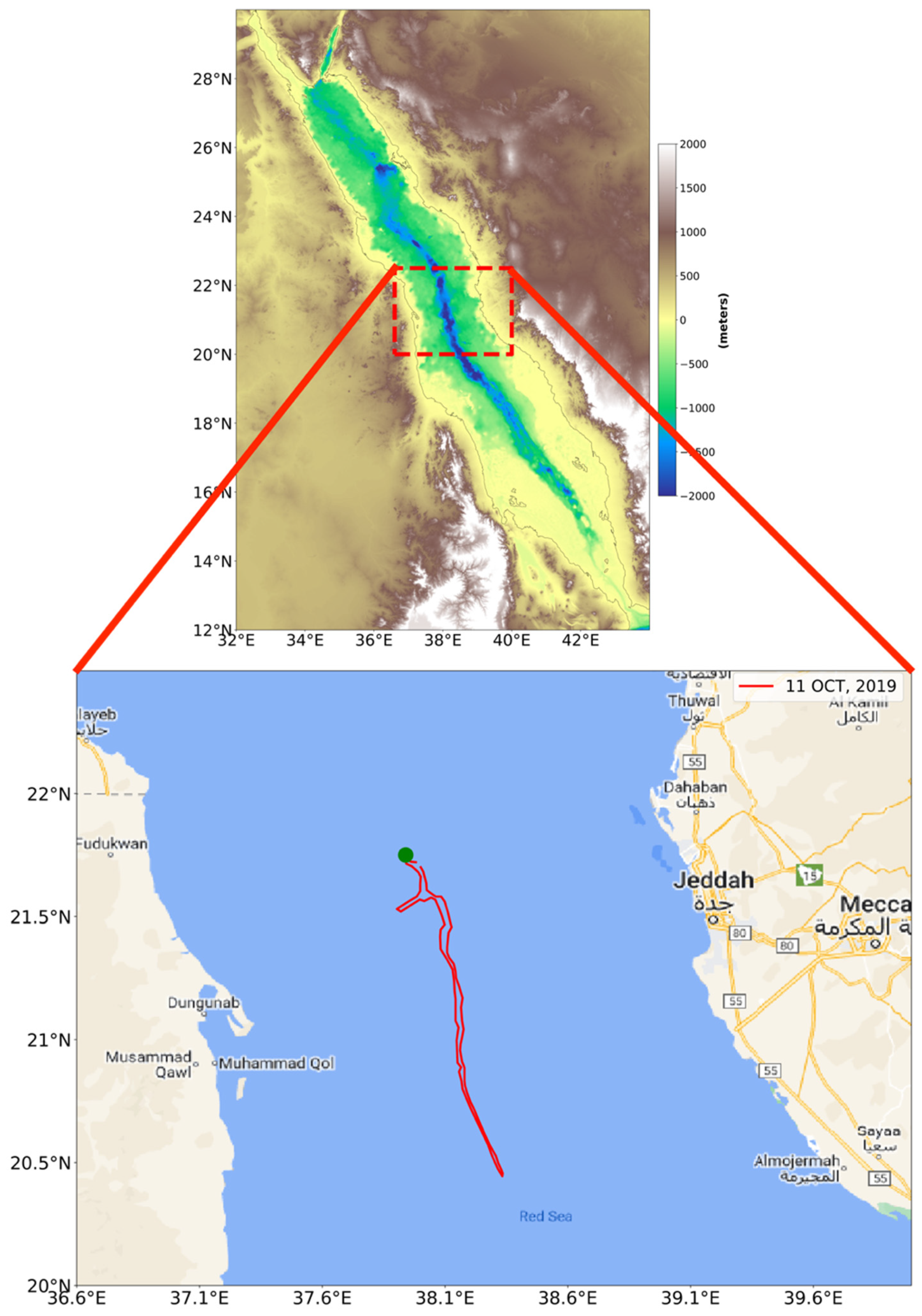
2. Data and Methods
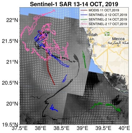
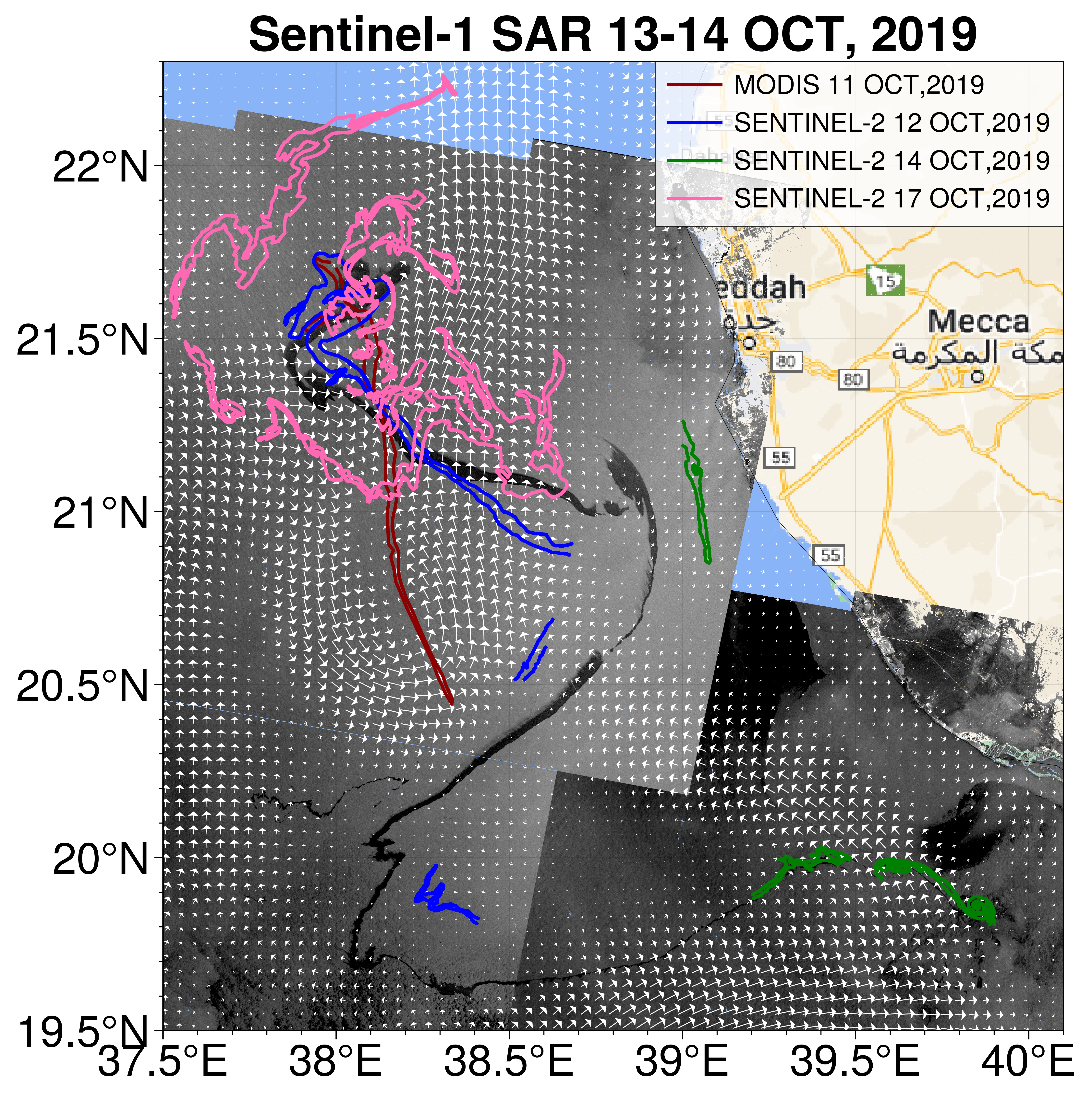
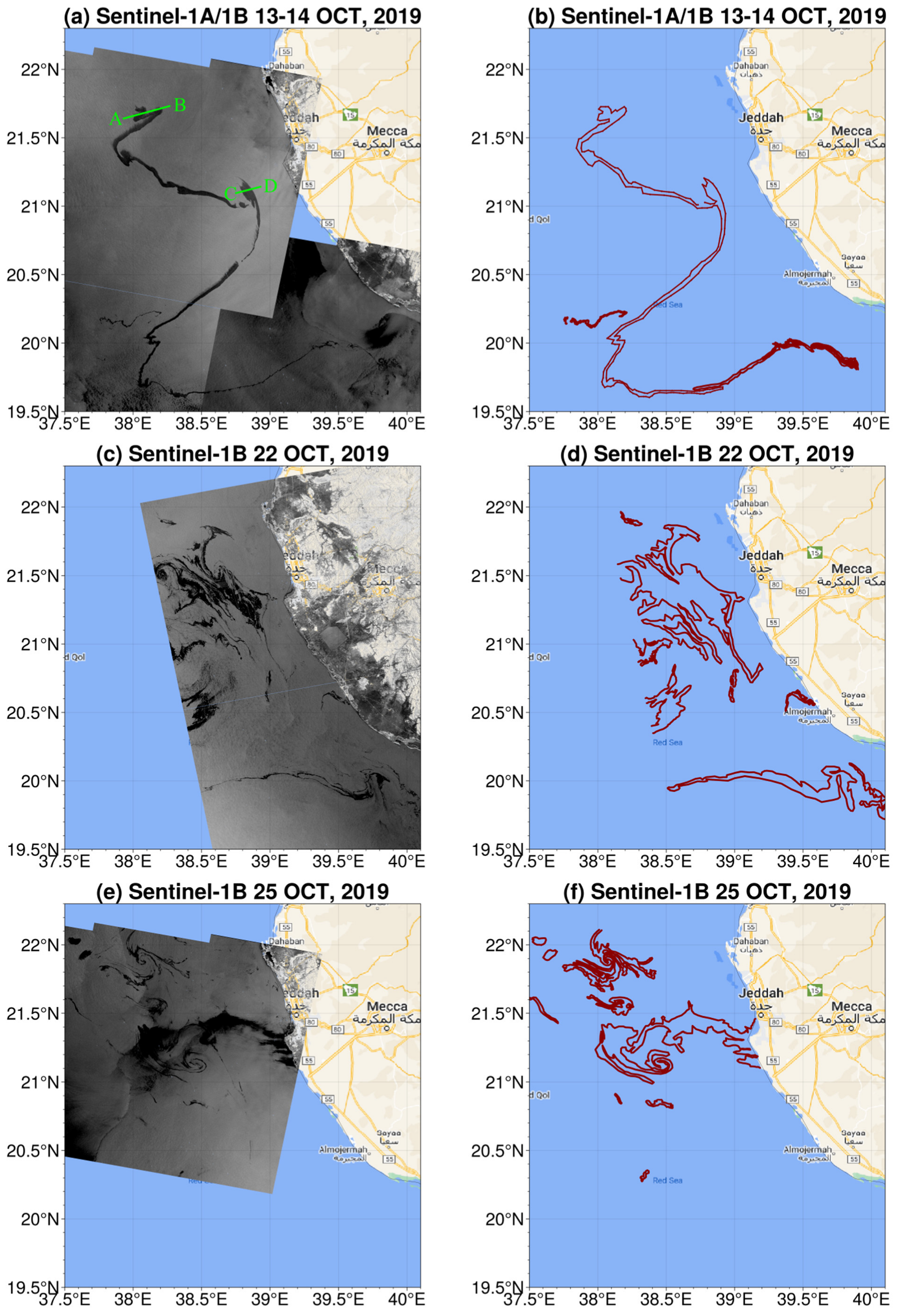
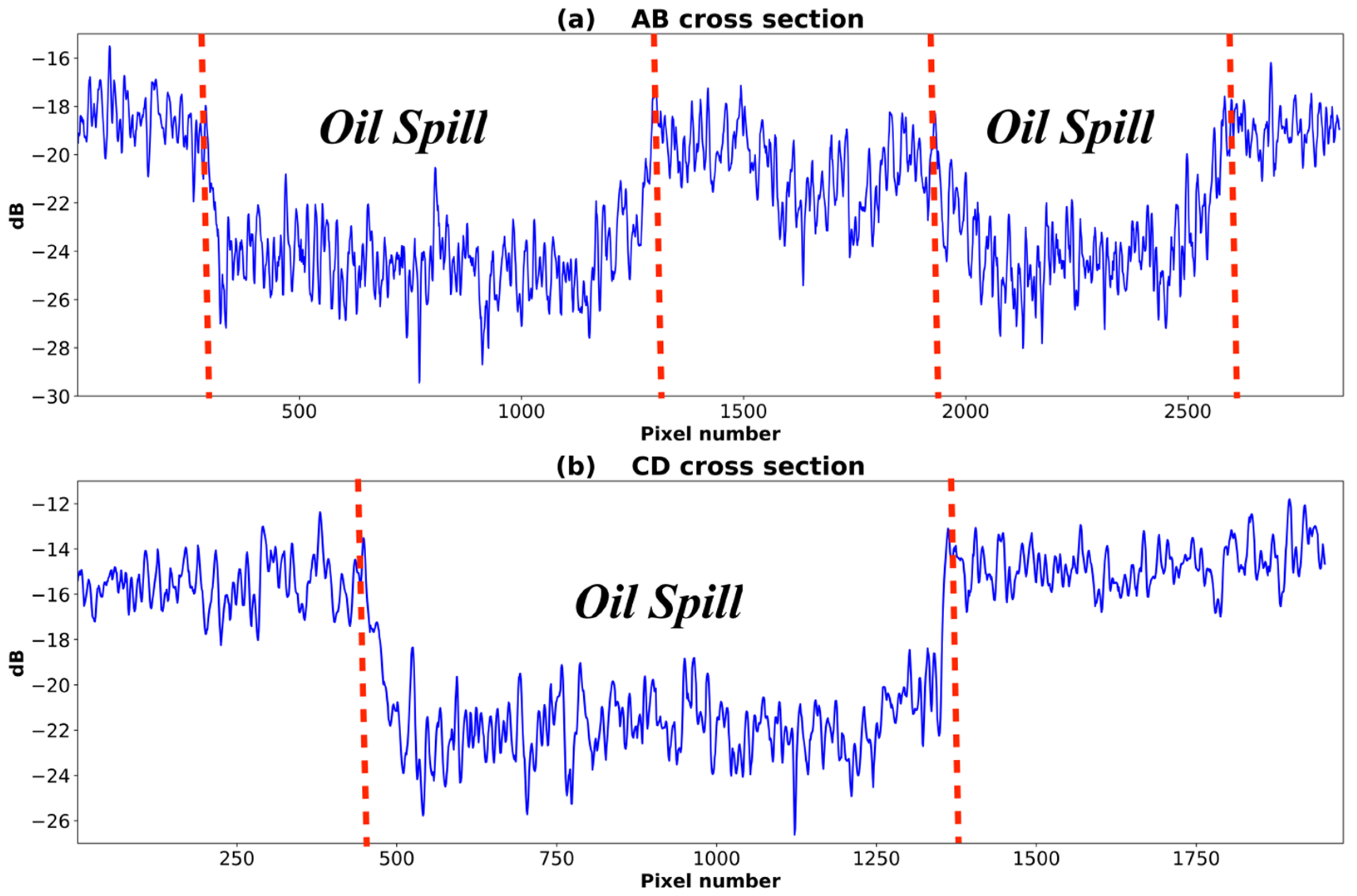
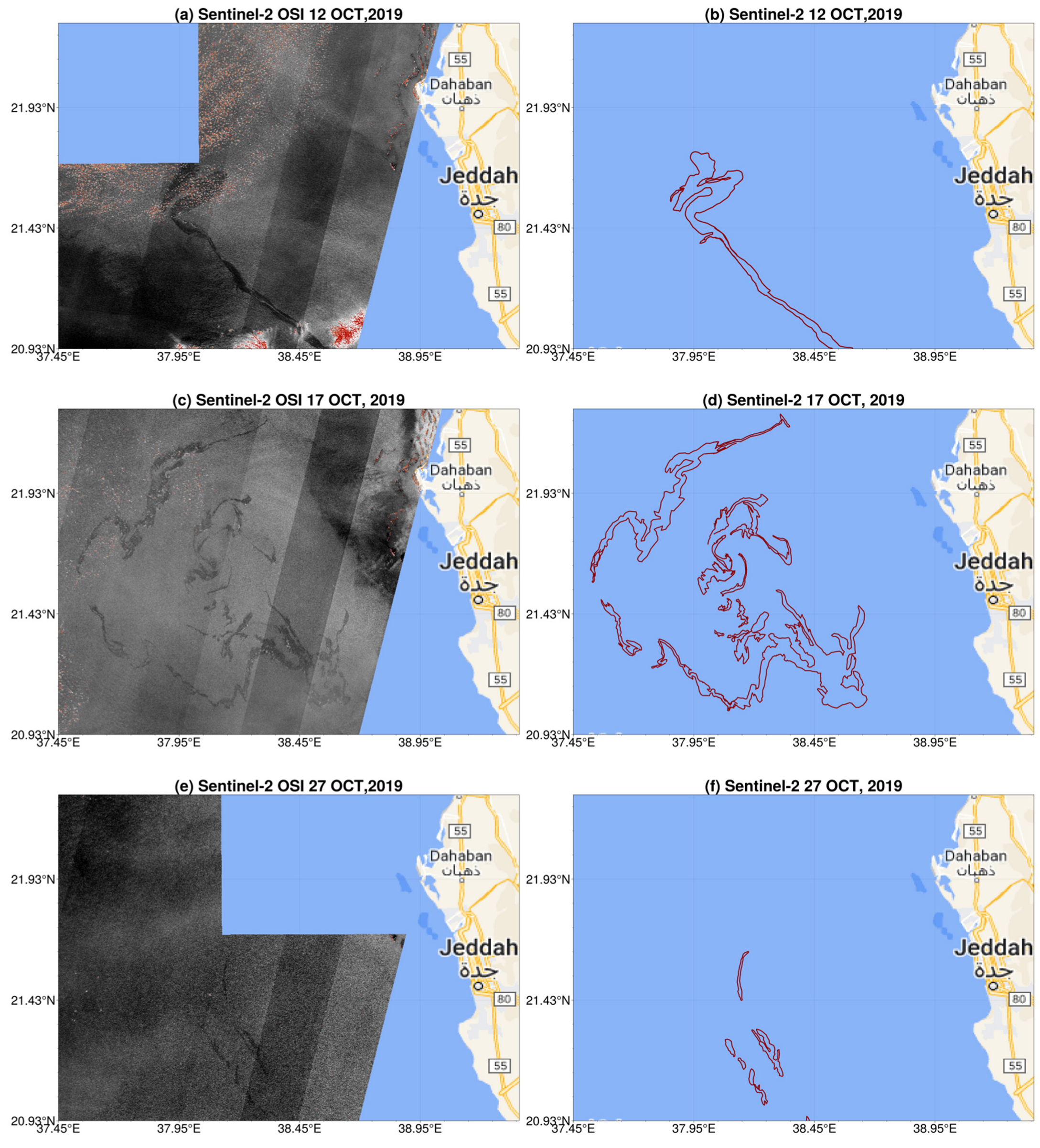
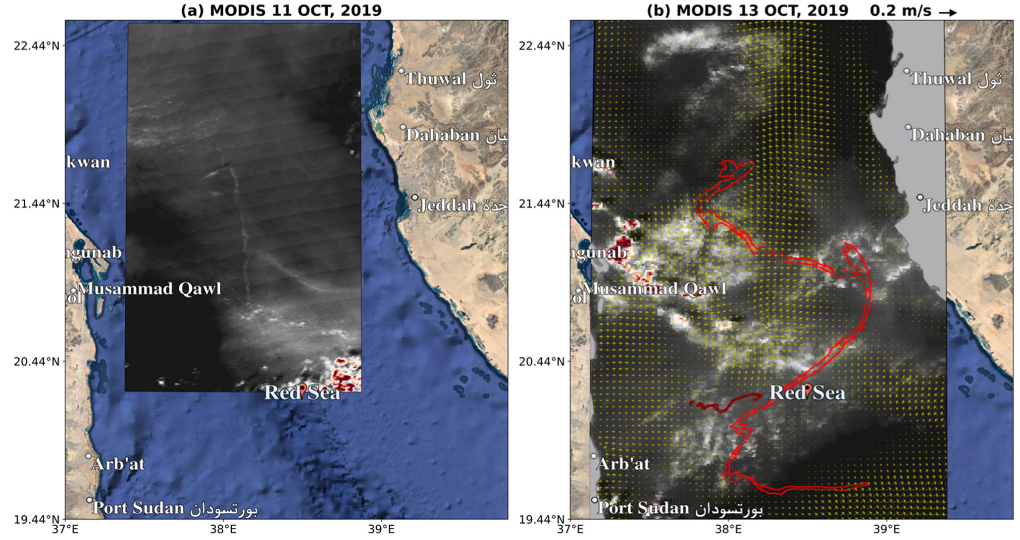
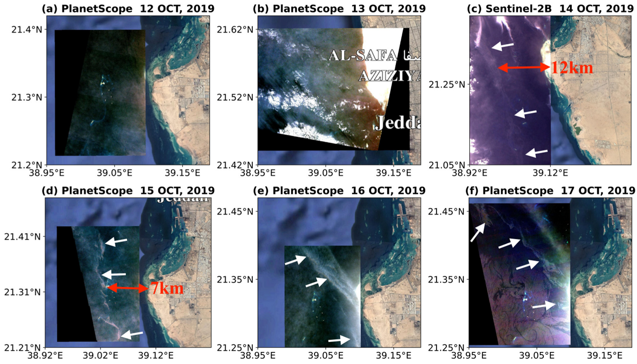
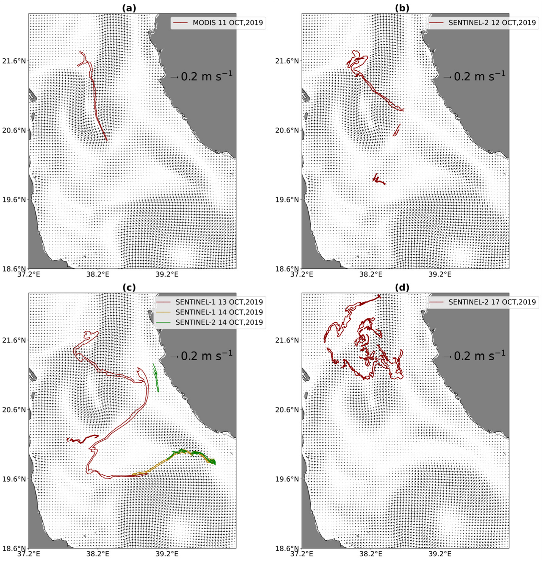
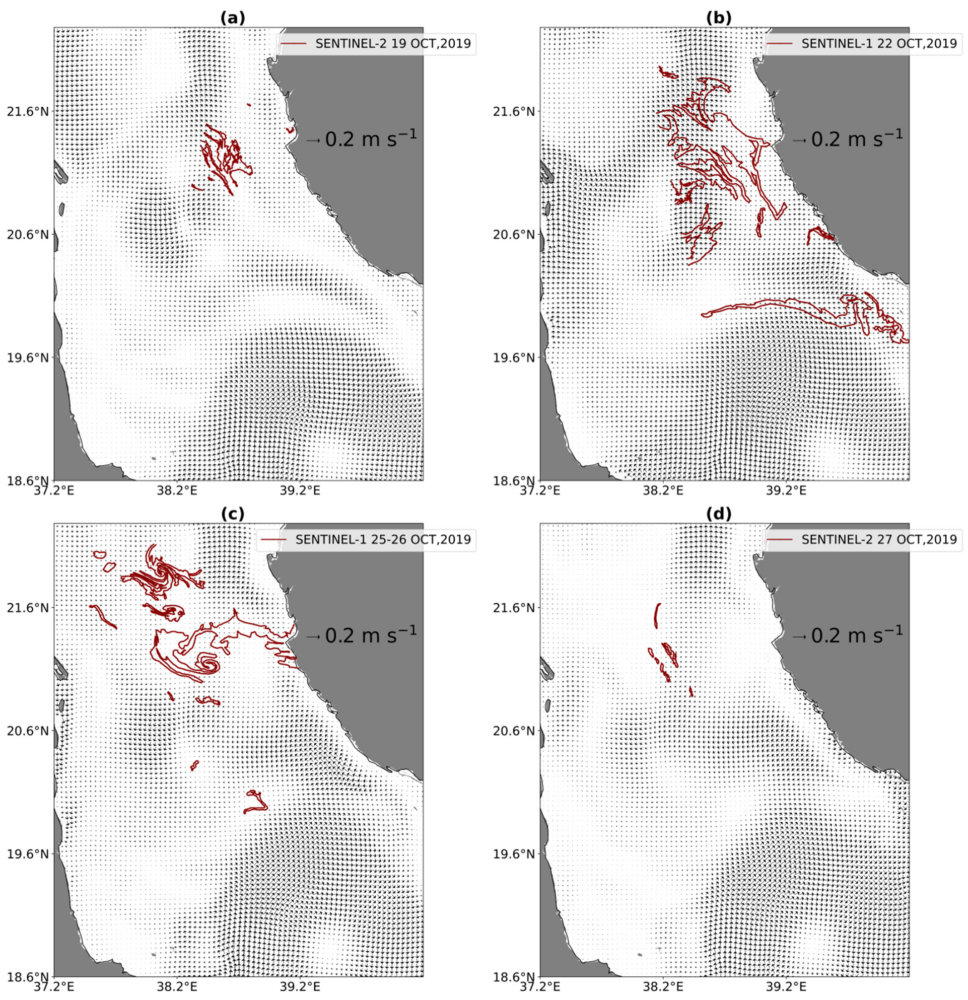
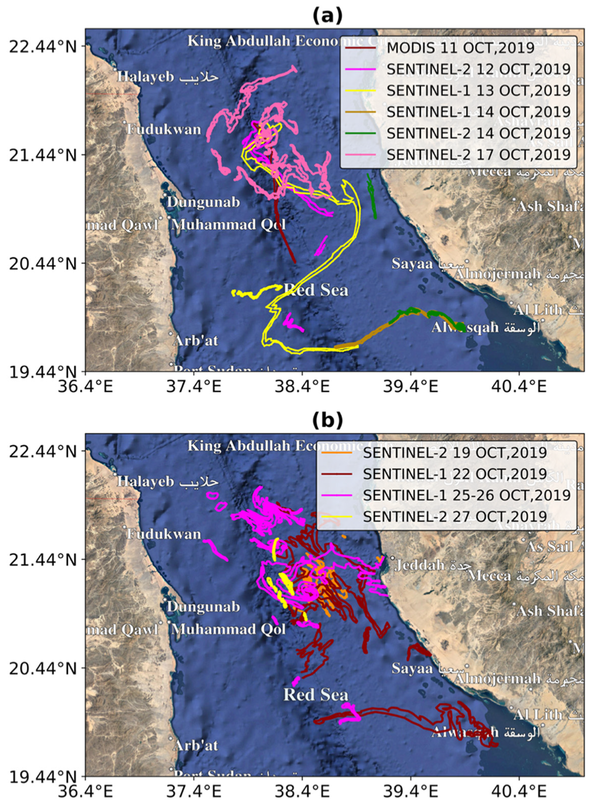
3. Remote Sensing RSOS-2019
4. Analysis of the Inferred Oil Spill Movement in Relation to Ocean Currents
5. Summary and Conclusions
Author Contributions
Funding
Data Availability Statement
Acknowledgments
Conflicts of Interest
References
- De Moura, N.V.A.; de Carvalho, O.L.F.; Gomes, R.A.T.; Guimarães, R.F.; de Carvalho Júnior, O.A. Deep-water oil-spill monitoring and recurrence analysis in the Brazilian territory using Sentinel-1 time series and deep learning. Int. J. Appl. Earth Obs. Geoinf. 2022, 107, 102695. [Google Scholar] [CrossRef]
- Fartoosi, F.M.; Fartoosi, A.; Fartoosi, F.M.; Fartoosi, A. The Impact of Maritime Oil Pollution in the Marine Environment: Case Study of Maritime Oil Pollution in the Navigational Channel of Shatt Al-Arab. 2013. Available online: https://commons.wmu.se/all_dissertations/318/ (accessed on 21 October 2020).
- iTop Federation. Oil Tanker Spill Statistics 2019. Available online: https://www.itopf.org/knowledge-resources/data-statistics/statistics/ (accessed on 24 June 2021).
- Al-Ruzouq, R.; Gibril, M.B.A.; Shanableh, A.; Kais, A.; Hamed, O.; Al-Mansoori, S.; Khalil, M.A. Sensors, features, and machine learning for oil spill detection and monitoring: A review. Remote Sens. 2020, 12, 3338. [Google Scholar] [CrossRef]
- Hoteit, I.; Abualnaja, Y.; Afzal, S.; Ait-El-Fquih, B.; Akylas, T.; Antony, C.; Dawson, C.; Asfahani, K.; Brewin, R.J.; Cavaleri, L.; et al. Towards an end-to-end analysis and prediction system for weather, climate, and Marine applications in the Red Sea. Bull. Am. Meteorol. Soc. 2021, 102, E99–E122. [Google Scholar] [CrossRef]
- Essa, S.; Harahsheh, H.; Shiobara, M.; Nishidai, T. Operational remote sensing for the detection and monitoring of oil pollution in the Arabian gulf: Case studies from the United Arab Emirates. Dev. Earth Environ. Sci. 2005, 3, 31–48. [Google Scholar]
- Zodiatis, G.; Lardner, R.; Spanoudaki, K.; Sofianos, S.; Radhakrishnan, H.; Coppini, G.; Liubartseva, S.; Kampanis, N.; Krokos, G.; Hoteit, I.; et al. Operational oil spill modelling assessments. In Marine Hydrocarbon Spill Assessments; Elsevier: Amsterdam, The Netherlands, 2021; pp. 145–197. [Google Scholar]
- El-Magd, I.A.; Zakzouk, M.; Abdulaziz, A.M.; Ali, E.M. The potentiality of operational mapping of oil pollution in the mediterranean sea near the entrance of the Suez canal using sentinel-1 SAR data. Remote Sens. 2020, 12, 1352. [Google Scholar] [CrossRef] [Green Version]
- Huynh, B.Q.; Kwong, L.H.; Kiang, M.V.; Chin, E.T.; Mohareb, A.M.; Jumaan, A.O.; Basu, S.; Geldsetzer, P.; Karaki, F.M.; Rehkopf, D.H. Public health impacts of an imminent Red Sea oil spill. Nat. Sustain. 2021, 4, 1084–1091. [Google Scholar] [CrossRef] [PubMed]
- Mittal, H.V.R.; Langodan, S.; Zhan, P.; Li, S.; Knio, O.; Hoteit, I. Hazard assessment of oil spills along the main shipping lane in the Red Sea. Sci. Rep. 2021, 11, 17078. [Google Scholar] [CrossRef] [PubMed]
- Gianinetto, M.; Maianti, P.; Tortini, R.; Nodari, F.; Lechi, G. Evaluation of MODIS data for mapping oil slicks-the Deepwater Horizon oil spill case. In Geographic Technologies Applied to Marine Spatial Planning and Integrated Coastal Zone Management; Universidade Dos Açores: Ponta Delgada, Portugal, 2010; pp. 61–67. [Google Scholar]
- Nukapothula, S.; Wu, J.; Chen, C.; Ali, P.Y. Potential impact of the extensive oil spill on primary productivity in the Red Sea waters. Cont. Shelf Res. 2021, 222, 104437. [Google Scholar] [CrossRef]
- Li, Y.; Cui, C.; Liu, Z.; Liu, B.; Xu, J.; Zhu, X.; Hou, Y. Detection and monitoring of oil spills using moderate/high-resolution remote sensing images. Arch. Environ. Contam. Toxicol. 2017, 73, 154–169. [Google Scholar] [CrossRef] [PubMed]
- Arslan, N. Assessment of oil spills using Sentinel 1 C-band SAR and Landsat 8 multispectral sensors. Environ. Monit. Assess. 2018, 190, 637. [Google Scholar] [CrossRef]
- Jha, M.N.; Levy, J.; Gao, Y. Advances in remote sensing for oil spill disaster management: State-of-the-art sensors technology for oil spill surveillance. Sensors 2008, 8, 236–255. [Google Scholar] [CrossRef] [PubMed]
- Leifer, I.; Lehr, W.J.; Simecek-Beatty, D.; Bradley, E.; Clark, R.; Dennison, P.; Hu, Y.; Matheson, S.; Jones, C.E.; Holt, B.; et al. State of the art satellite and airborne marine oil spill remote sensing: Application to the BP Deepwater Horizon oil spill. Remote Sens. Environ. 2012, 124, 185–209. [Google Scholar] [CrossRef] [Green Version]
- Sun, S.; Hu, C.; Garcia-Pineda, O.; Kourafalou, V.; Le Hénaff, M.; Androulidakis, Y. Remote sensing assessment of oil spills near a damaged platform in the Gulf of Mexico. Mar. Pollut. Bull. 2018, 136, 141–151. [Google Scholar] [CrossRef]
- Maianti, P.; Rusmini, M.; Tortini, R.; Dalla Via, G.; Frassy, F.; Marchesi, A.; Rota Nodari, F.; Gianinetto, M. Monitoring large oil slick dynamics with moderate resolution multispectral satellite data. Nat. Hazards 2014, 73, 473–492. [Google Scholar] [CrossRef]
- Della Torre, C.; Tornambè, A.; Cappello, S.; Mariottini, M.; Perra, G.; Giuliani, S.; Amato, E.; Falugi, C.; Crisari, A.; Yakimov, M.M.; et al. Modulation of CYP1A and genotoxic effects in European seabass (Dicentrarchus labrax) exposed to weathered oil: A mesocosm study. Mar. Environ. Res. 2012, 76, 48–55. [Google Scholar] [CrossRef] [PubMed]
- Ivanov, A.; He, M.; Fang, M. Oil spill detection with the RADARSAT SAR in the waters of the Yellow and East China Sea: A case study. In Proceedings of the 23rd Asian Conferrence on Remote Sensing, Kathmandu, Nepal, 25–29 November 2002. [Google Scholar]
- Keramea, P.; Spanoudaki, K.; Zodiatis, G.; Gikas, G.; Sylaios, G. Oil spill modeling: A critical review on current trends, perspectives, and challenges. J. Mar. Sci. Eng. 2021, 9, 181. [Google Scholar] [CrossRef]
- Kolokoussis, P.; Karathanassi, V. Oil spill detection and mapping using sentinel 2 imagery. J. Mar. Sci. Eng. 2018, 6, 4. [Google Scholar] [CrossRef] [Green Version]
- Nezhad, M.M.; Groppi, D.; Marzialetti, P.; Piras, G.; Laneve, G. Mapping sea water surface in Persian Gulf, oil spill detection using Sentinal-1 images. In Proceedings of the 4th World Congress on New Technologies, Madrid, Spain, 19–21 August; 2018; pp. 19–21. [Google Scholar]
- Rajendran, S.; Vethamony, P.; Sadooni, F.N.; Al-Kuwari, H.A.S.; Al-Khayat, J.A.; Govil, H.; Nasir, S. Sentinel-2 image transformation methods for mapping oil spill—A case study with Wakashio oil spill in the Indian Ocean, off Mauritius. MethodsX 2021, 8, 101327. [Google Scholar] [CrossRef]
- Marghany, M.; Cracknell, A.P.; Hashim, M. Modification of fractal algorithm for oil spill detection from RADARSAT-1 SAR data. Int. J. Appl. Earth Obs. Geoinf. 2009, 11, 96–102. [Google Scholar] [CrossRef] [Green Version]
- Guo, Y.; Zhang, H.Z. Oil spill detection using synthetic aperture radar images and feature selection in shape space. Int. J. Appl. Earth Obs. Geoinf. 2014, 30, 146–157. [Google Scholar] [CrossRef]
- Fingas, M.; Brown, C.E. A review of oil spill remote sensing. Sensors 2018, 18, 91. [Google Scholar] [CrossRef] [PubMed]
- Fingas, M.; Brown, C. Review of oil spill remote sensing. Mar. Pollut. Bull. 2014, 83, 9–23. [Google Scholar] [CrossRef] [PubMed] [Green Version]
- Fingas, M.; Brown, C.E. Oil Spill Remote Sensing: A Review. Oil Spill Science and Technology; Gulf Professional Publishing: Boston, MA, USA, 2011; pp. 111–169. [Google Scholar]
- Hu, C.; Li, X.; Pichel, W.G. Detection of Oil Slicks using MODIS and SAR Imagery. IOCCG Rep. 2006, 5, 14. [Google Scholar]
- Zhao, J.; Temimi, M.; Ghedira, H.; Hu, C. Exploring the potential of optical remote sensing for oil spill detection in shallow coastal waters-a case study in the Arabian Gulf. Opt. Express 2014, 22, 13755. [Google Scholar] [CrossRef]
- Times, Iran Says Oil Tanker Hit by Two Missiles off SAUDI Arabia Coast|Financial. Available online: https://www.ft.com/content/2ae8d55a-ebef-11e9-a240-3b065ef5fc55 (accessed on 24 December 2021).
- National, T. Iran Claims Oil Tanker Attacked in the Red Sea. Available online: https://www.thenationalnews.com/world/mena/iran-claims-oil-tanker-attacked-in-the-red-sea-1.922005 (accessed on 24 December 2021).
- Yekeen, S.T.; Balogun, A.L. Advances in remote sensing technology, machine learning and deep learning for marine oil spill detection, prediction, and vulnerability assessment. Remote Sens. 2020, 12, 3416. [Google Scholar] [CrossRef]
- Yang, Y.J.; Singha, S.; Mayerle, R. A deep learning based oil spill detector using Sentinel-1 SAR imagery. Int. J. Remote Sens. 2022, 43, 4287–4314. [Google Scholar] [CrossRef]
- Alpers, W.; Holt, B.; Zeng, K. Oil spill detection by imaging radars: Challenges and pitfalls. Remote Sens. Environ. 2017, 201, 133–147. [Google Scholar] [CrossRef]
- Dong, Y.; Liu, Y.; Hu, C.; MacDonald, I.R.; Lu, Y. Chronic oiling in global oceans. Science 2022, 376, 1300–1304. [Google Scholar] [CrossRef]
- Filipponi, F. Sentinel-1 GRD Preprocessing Workflow. Proceedings 2019, 18, 11. [Google Scholar]
- Topouzelis, K.N. Oil spill detection by SAR images: Dark formation detection, feature extraction and classification algorithms. Sensors 2008, 8, 6642–6659. [Google Scholar] [CrossRef] [Green Version]
- Rajendran, S.; Vethamony, P.; Sadooni, F.N.; Al-Kuwari, H.A.S.; Al-Khayat, J.A.; Seegobin, V.O.; Govil, H.; Nasir, S. Detection of Wakashio oil spill off Mauritius using Sentinel-1 and 2 data: Capability of sensors, image transformation methods, and mapping. Environ. Pollut. 2021, 274, 116618. [Google Scholar] [CrossRef] [PubMed]
- Brekke, C.; Solberg, A.H.S. Oil spill detection by satellite remote sensing. Remote Sens. Environ. 2005, 95, 1–13. [Google Scholar] [CrossRef]
- Garcia-Pineda, O.; Staples, G.; Jones, C.E.; Hu, C.; Holt, B.; Kourafalou, V.; Graettinger, G.; DiPinto, L.; Ramirez, E.; Streett, D.; et al. Classification of oil spill by thicknesses using multiple remote sensors. Remote Sens. Environ. 2020, 236, 111421. [Google Scholar] [CrossRef]
- Moskolaï, W.R.; Abdou, W.; Dipanda, A. A Workflow for Collecting and Preprocessing Sentinel-1 Images for Time Series Prediction Suitable for Deep Learning Algorithms. Geomatics 2022, 2, 435–456. [Google Scholar] [CrossRef]
- Caballero, I.; Román, A.; Tovar-Sánchez, A.; Navarro, G. Water quality monitoring with Sentinel-2 and Landsat-8 satellites during the 2021 volcanic eruption in La Palma (Canary Islands). Sci. Total Environ. 2022, 822, 153433. [Google Scholar] [CrossRef] [PubMed]
- Sanikommu, S.; Toye, H.; Zhan, P.; Langodan, S.; Krokos, G.; Knio, O.; Hoteit, I. Impact of atmospheric and model physics perturbations on a high-resolution ensemble data assimilation system of the Red Sea. J. Geophys. Res. Oceans 2020, 125, 8. [Google Scholar] [CrossRef]
- Sanikommu, S.; Banerjee, D.S.; Baduru, B.; Paul, B.; Paul, A.; Chakraborty, K.; Hoteit, I. Impact of dynamical representational errors on an Indian Ocean ensemble data assimilation system. Q. J. R. Meteorol. Soc. 2019, 145, 3680–3691. [Google Scholar] [CrossRef]
- Sanikommu, S.R.; Langodan, S.; Dasari, H.P.; Zhan, P.; Krokos, G.; Abualnaja, Y.O.; Asfahani, K.; Hoteit, I. Making the case for high resolution regional reanalyses: An example with the Red Sea. Bull. Am. Meteorol. Soc. 2022; under review. [Google Scholar]
- Toye, H.; Sanikommu, S.; Raboudi, N.F.; Hoteit, I. A hybrid ensemble adjustment Kalman filter based high-resolution data assimilation system for the Red Sea: Implementation and evaluation. Q. J. R. Meteorol. Soc. 2020, 146, 4108–4130. [Google Scholar] [CrossRef]
- Klemas, V. Tracking oil slicks and predicting their trajectories using remote sensors and models: Case studies of the Sea Princess and Deepwater Horizon oil spills. J. Coast. Res. 2010, 265, 789–797. [Google Scholar] [CrossRef] [Green Version]
- Pan, Q.; Yu, H.; Daling, P.S.; Zhang, Y.; Reed, M.; Wang, Z.; Li, Y.; Wang, X.; Wu, L.; Zhang, Z.; et al. Fate and behavior of Sanchi oil spill transported by the Kuroshio during January–February 2018. Mar. Pollut. Bull. 2020, 152, 110917. [Google Scholar] [CrossRef]
- Rao, V.T.; Suneel, V.; Alex, M.J.; Gurumoorthi, K.; Thomas, A.P. Assessment of MV Wakashio oil spill off Mauritius, Indian Ocean through satellite imagery: A case study. J. Earth Syst. Sci. 2022, 131, 21. [Google Scholar] [CrossRef]
- Patzert, W.C. Wind-induced reversal in Red Sea circulation. Deep Sea Res. Oceanogr. Abstr. 1974, 21, 109–121. [Google Scholar] [CrossRef]
- Patlakas, P.; Stathopoulos, C.; Flocas, H.; Kalogeri, C.; Kallos, G. Regional climatic features of the Arabian Peninsula. Atmosphere 2019, 10, 220. [Google Scholar] [CrossRef]
- Alharbi, F.R.; Csala, D. Gulf cooperation council countries’ climate change mitigation challenges and exploration of solar and wind energy resource potential. Appl. Sci. 2021, 11, 2648. [Google Scholar] [CrossRef]
- Sofianos, S.S.; Johns, W.E. An Oceanic General Circulation Model (OGCM) investigation of the red sea circulation: 2. Three-dimensional circulation in the Red Sea. J. Geophys. Res. Oceans 2003, 108, 1–15. [Google Scholar] [CrossRef] [Green Version]
- Yao, F.; Hoteit, I.; Pratt, L.J.; Bower, A.S.; Köhl, A.; Gopalakrishnan, G.; Rivas, D. Seasonal overturning circulation in the Red Sea: 2. Winter circulation. J. Geophys. Res. Oceans 2014, 119, 2238–2262. [Google Scholar] [CrossRef] [Green Version]
- Zhai, P.; Pratt, L.J.; Bower, A. On the crossover of boundary currents in an idealized model of the Red sea. J. Phys. Oceanogr. 2015, 45, 1410–1425. [Google Scholar] [CrossRef]
- Bower, A.S.; Farrar, J.T. Air–Sea Interaction and Horizontal Circulation in the Red Sea; Springer Earth System Sciences; Springer: Berlin/Heidelberg, Germany, 2015; pp. 329–342. [Google Scholar]
- Zhan, P.; Gopalakrishnan, G.; Subramanian, A.C.; Guo, D.; Hoteit, I. Sensitivity Studies of the Red Sea Eddies Using Adjoint Method. J. Geophys. Res. Oceans 2018, 123, 8329–8345. [Google Scholar] [CrossRef] [Green Version]
- Zhai, P.; Bower, A. The response of the Red Sea to a strong wind jet near the Tokar Gap in summer. J. Geophys. Res. Oceans 2013, 118, 421–434. [Google Scholar] [CrossRef]
- Zhan, P.; Subramanian, A.C.; Yao, F.; Kartadikaria, A.R.; Guo, D.; Hoteit, I. The eddy kinetic energy budget in the Red Sea. J. Geophys. Res. Oceans 2016, 121, 4732–4747. [Google Scholar] [CrossRef] [Green Version]
- Krestenitis, M.; Orfanidis, G.; Ioannidis, K.; Avgerinakis, K.; Vrochidis, S.; Kompatsiaris, I. Oil spill identification from satellite images using deep neural networks. Remote Sens. 2019, 11, 1762. [Google Scholar] [CrossRef] [Green Version]
- Li, B.; Xu, J.; Pan, X.; Ma, L.; Zhao, Z.; Chen, R.; Liu, Q.; Wang, H. Marine Oil Spill Detection with X-Band Shipborne Radar Using GLCM, SVM and FCM. Remote Sens. 2022, 14, 3715. [Google Scholar] [CrossRef]
- De Kerf, T.; Gladines, J.; Sels, S.; Vanlanduit, S. Oil spill detection using machine learning and infrared images. Remote Sens. 2020, 12, 4090. [Google Scholar] [CrossRef]
- Shaban, M.; Salim, R.; Khalifeh, H.A.; Khelifi, A.; Shalaby, A.; El-Mashad, S.; Mahmoud, A.; Ghazal, M.; El-Baz, A. A deep-learning framework for the detection of oil spills from SAR data. Sensors 2021, 21, 2351. [Google Scholar] [CrossRef] [PubMed]


| Parameter | Interferometric Wide Swath Mode (IW) |
|---|---|
| Swath width | 250 km |
| Incident angle range | 29.1–46.0° |
| Sub-swaths | 3 |
| Azimuth steering angle | ±0.6° |
| Azimuth and range look | Single |
| Polarization | Dual VV + VH |
| Maximum Noise Equivalent Sigma Zero | −22 dB |
| Radiometric stability | 0.5 dB (3 ) |
| Pixel size (meter) | 10 |
| Satellite | Date | Image |
|---|---|---|
| Sentinel 1B | 13 October 2019 | S1B_IW_GRDH_1SDV_018451_022C28_AA13 |
| Sentinel 1B | 13 October 2019 | S1B_IW_GRDH_1SDV_018451_022C28_9E30 |
| Sentinel 1A | 14 October 2019 | S1A_IW_GRDH_1SDV_029449_03598E_1B6C |
| Sentinel 1B | 22 October 2019 | S1B_IW_GRDH_1SDV_018590_023066_0FFE |
| Sentinel 1B | 22 October 2019 | S1B_IW_GRDH_1SDV_018590_023066_ECE4 |
| Sentinel 1B | 25 October 2019 | S1B_IW_GRDH_1SDV_018626_023181_36B9 |
| Sentinel 1A | 26 October 2019 | S1A_IW_GRDH_1SDV_029624_035F8D_0944 |
| Operator | Parameter | Value |
|---|---|---|
| Read | Data format | Any format |
| Apply orbit file | Orbit state vectors Polynomial degree | Sentinel precise 3 |
| Calibration | Polarizations Output sigma0 band | VH, VV True |
| Terrain correction | Source bands band DEM DEM resampling method Image resampling method Pixel spacing | Sigma0_VH, Sigma0_VV SRTM 1Sec HGT (Auto Download) Bilinear interpolation Bilinear interpolation 10 m |
| Speckle filtering | Source band Filter | VV Refined Lee |
| Convert to dB | Source bands | VV |
| Write | Save as | GeoTIFF—BigTIFF |
| Satellite | Spectral Region (Bands) | Range (µm) | Spatial Resolution | Revisit Time | Operation | Level |
|---|---|---|---|---|---|---|
| MODIS (Aqua) | VIS, NIR, MIR, SWIR, LWIR (36 bands) | B1-19 (0.405–2.155), B20-36 (3.66–14.28) | 250, 500, 1000 m | 1–2 day | 2002 | L1B |
| Landsat-8 | VIS, NIR, SWIR, TIR (12 bands) | B1-9 (0.43–1.38), B10-11 (10.6–12.51) | 15, 30, 100 m | 16 day | 2013 | L1T |
| Meteosat | VIS, NIR, IR, HRV | B1-3 (0.6–1.7) B4-11 (3.8–14) B12 (0.5–0.9) | 3 km, 1000 m | 15 min | 2002 | Level 1.5 |
| PlanetScope | VIS, NIR (4 bands) | B1 (0.45–0.51) B2 (0.50–0.59) B3 (0.59–0.67) B4 (0.73–0.74) B5 (0.78–0.86) | 3 m | Daily | 2016 | PS2 |
| Sentinel-2 | VIS, NIR, SWIR (12 bands) | 0.443–2.190 | 10, 20, 60 m | 5 day | 2015 | L1C |
Disclaimer/Publisher’s Note: The statements, opinions and data contained in all publications are solely those of the individual author(s) and contributor(s) and not of MDPI and/or the editor(s). MDPI and/or the editor(s) disclaim responsibility for any injury to people or property resulting from any ideas, methods, instructions or products referred to in the content. |
© 2022 by the authors. Licensee MDPI, Basel, Switzerland. This article is an open access article distributed under the terms and conditions of the Creative Commons Attribution (CC BY) license (https://creativecommons.org/licenses/by/4.0/).
Share and Cite
Vankayalapati, K.; Dasari, H.P.; Langodan, S.; El Mohtar, S.; Sanikommu, S.; Asfahani, K.; Desamsetti, S.; Hoteit, I. Multi-Mission Satellite Detection and Tracking of October 2019 Sabiti Oil Spill in the Red Sea. Remote Sens. 2023, 15, 38. https://doi.org/10.3390/rs15010038
Vankayalapati K, Dasari HP, Langodan S, El Mohtar S, Sanikommu S, Asfahani K, Desamsetti S, Hoteit I. Multi-Mission Satellite Detection and Tracking of October 2019 Sabiti Oil Spill in the Red Sea. Remote Sensing. 2023; 15(1):38. https://doi.org/10.3390/rs15010038
Chicago/Turabian StyleVankayalapati, Koteswararao, Hari Prasad Dasari, Sabique Langodan, Samah El Mohtar, Sivareddy Sanikommu, Khaled Asfahani, Srinivas Desamsetti, and Ibrahim Hoteit. 2023. "Multi-Mission Satellite Detection and Tracking of October 2019 Sabiti Oil Spill in the Red Sea" Remote Sensing 15, no. 1: 38. https://doi.org/10.3390/rs15010038