Article

Bouguer Anomaly Re-Reduction and Interpretative Remarks of the Phlegraean Fields Caldera Structures (Southern Italy)

1
National Institute of Geophysics and Volcanology (INGV), Environment Department-Roma 2, 00143 Roma, Italy
2
ISMAR-CNR National Research Council of Italy, 80133 Naples, Italy
3
Mira Geoscience Ltd., Vancouver, BC V6C 1T2, Canada
4
Eni Spa—Natural Resources, San Donato Milanese, 20097 Milan, Italy
*
Author to whom correspondence should be addressed.
Remote Sens. 2023, 15(1), 209; https://doi.org/10.3390/rs15010209
Submission received: 27 October 2022 / Revised: 16 December 2022 / Accepted: 21 December 2022 / Published: 30 December 2022

Abstract

:
Phlegraean Fields is a large, active caldera located in the densely populated westernmost sector of Naples’s Bay (Southern Italy). Several Bouguer anomaly surveys are available for this area with different resolution and accuracy; gravity data derive from the integration of stations placed below and above the sea level as the caldera develops both onshore and offshore. The comparison of these maps with the Digital Elevation Model shows a still remaining Terrain Effect hiding the shallower and deep caldera structure’s signal. This effect has an impact on the modelling of the gravity source’s depth and geometry. In this research, we apply a geologically constrained terrain correction method to the higher resolution Free Air dataset available for the study area to enhance the complete Bouguer reduction. The correlation analysis between the residual and the topography allows us to assess the quality of the outcomes. The results represent an improvement in the anomalies’ isolation and clearly show a continuous circular-like clustering of maxima related to the geometry of the caldera rim. The minima are associated with volcano-tectonic depression filled with pyroclastic and sediment. Furthermore, features alignments overlap the fault systems, along which the volcanic activity occurred.

1. Introduction

The analysis of gravity data allows us to investigate the subsurface in different geo-tectonic environments, from surficial shallower to very deep crustal layers. This is especially true in volcanic environments because of the occurrence of strong rock property contrasts among the different volcanic products (e.g., intrusive dikes, lava flows, scoria cones, etc.). In this paper, we consider the gravity signature of the Phlegraean Fields caldera (hereafter CFc). This wide caldera structure derived from two major eruptions that occurred at 39 ka and 15 ka [1,2], emplacing the so-called “Campanian Ignimbrite” (IC) and “Neapolitan Yellow Tuff” (NYT) [3,4,5], respectively, and from a potential third event that occurred at ca. 29 ka [6].
The published Bouguer anomalies maps of the CFc area show an overall subsampling of the gravity features, partially covering the whole caldera extension, and somewhere they also show an evident correlation with the topography. All maps display a sub-circular gravity minimum, with the lowest values occurring in the central sector of the caldera. This minimum is interpreted as the effect of the sedimentary infilling of the depression, whose bottom is placed at about 3 km depth [7].
Nunziata and Rapolla [8], using old on-land and marine data, propose two alternative hypotheses about the nature of the Bouguer anomalies characterizing the CFc area. The study assumes the presence of material with different densities inside and outside the caldera and/or of a molten magmatic reservoir at shallower depths. Cassano and La Torre [9] propose a detailed description, analysis and modelling of gravimetric data aimed at reconstructing the CFc volcanological history. In this study, the authors use the data coming from the AGIP and Italian Geological Survey database, characterized by a good resolution of the CP inland areas and a poor resolution for the marine sectors.
A higher resolution dataset that also includes the CFc offshore was published by Barberi et al. [3]. These authors propose a structural model on the basis of a 2.5 D forward modelling of the Bouguer anomalies, computed along specific key profiles crossing the CFc area. The modelling uses rock density values that come from prospecting drill logs [9,10].
Florio et al. [11] applied the boundary analysis method to the higher-resolution datasets [9,12], depicting a new tectonic setting of the whole CP and CFc areas.
Berrino et al. [12,13] revealed the existence of a denser rock layer between 2 and 3 km of depth, which is interpreted as a water- and/or gas-bearing thermo-metamorphic sequence overlying the basement [14,15]. Seismic reflection data indicated the occurrence of the Mesozoic limestone basement at a depth ≥ 6 km [14], placed over a 1 km thick low-velocity layer at about 8 km depth, interpreted as the upper portion of a partially molten region [15]. Seismic attenuation in the tomographic data highlights the possible existence of a melt at a depth of 4–5 km, just beneath the central CFc sector, which uplifted during the 1982–1984 bradyseism [16]. Moreover, tomography data reveal a low Vp/Vs layer at about 2–2.5 km (high Qp and Qs) overlying a deeper high Vp/Vs (low Qp and Qs) region placed between 2.5–4 km [17]. The two layers were interpreted as a gas-saturated zone overlying conduits of fluid-enriched partially molten material.
Capuano et al. [18] assembled marine and terrestrial gravimetric datasets derived from different surveys [13,19,20], thus providing a new 3D inversion of the Free Air data to better model the architecture of the inner portion of the caldera.
The gravimetric studies described above are based on measurements carried out with different resolution and accuracy in the last decades of the twentieth century on the CFc area. All these works were aimed at the reconstruction of the caldera history through the modelling of its low/high frequency signals, derived from the depression and from the small-scale volcanic structures developed after the caldera formation.
The complete Bouguer reduction is the last step of the data processing obtained by removing the gravimetric effect induced by the local topography. A detailed analysis of the CFc Bouguer maps published up to now versus the high-resolution Digital Elevation Model highlights how, in some areas, the correlations between the gravimetric anomaly and the topographic features still remain in the data to varying degrees. More in general, this correlation is often caused by a unique reference density (topography density) used during the data processing for complete terrain correction [21]. Therefore, the Bouguer fields often still contain the contribution of the local Terrain Effect, especially where the chosen reference density considerably differs from the real one. As a consequence, in previous gravimetric surveys of Phlegraean Fields, the signal of the buried caldera is often partially obscured by the effects of the topographic sources. This condition has a significant impact on the successive quantitative estimation of the source’s depths and geometries (Figure 1).
In this work, we applied the complete Bouguer Reduction technique based on the prismatic mass approximation of the gravity signal. Therefore, we carried out the re-reduction of the high-resolution Phlegraean Fields Free Air anomaly datasets furnished by Eni S.p.A. (Ente Nazionale Idrocarburi) to obtain the Complete Bouguer Anomaly (CBA) map of the CFc area. To accomplish that, we considered a geologically constrained Forward Modelling based on the VPmg code [26,27], particularly useful when dealing with the TGE of articulated topography, as in the case of the Campanian Plain (CP), which extends from the pelagic depths of the Tyrrhenian Sea to the higher Apennine chain elevations.
Finally, we performed the correlation analysis between gravity and elevation (DEM), providing a scatter analysis of the two variables, as well as the statistical estimation of the correlation coefficient. These two approaches, supported by well-known geological features of the study area (stratigraphic sequence, local densities), provided the effectiveness of the complete CBA field reduction for the CFc area. This latter field is, therefore, compared with the regional Bouguer Anomaly derived by the “Progetto Finalizzato Geodinamica” (Italian National Research Council—CNR) available for the Italian country [28], in order to evaluate and remove (de-trend) the longer wavelength effects of the deeper-seated crustal sources. The obtained de-trended Bouguer map is compared with the previously published gravimetric maps [3,8,11], and its qualitative interpretation is provided in light of the stratigraphy characteristics and tectonic structures of the area (Figure 1). The overall analysis assesses an improvement in gravimetric data reduction and a better isolation of the signals, supplying a new updated map of the Phlegraean caldera Bouguer anomalies.

2. Geological Background

CFc lies in the western sector of Campanian Plain, which represents a NW–SE elongated, Plio-Quaternary structural depression, delimited to the east by NW–SE striking faults and to the north and south by NE–SW faults (Figure 1). Campanian Plain as shown by the digital elevation model of Figure 2 is bounded to the west by the Tyrrhenian Sea basin and to the east by Southern Apennines, which represent the fold-and-thrust belt associated with the westward subduction of the Apulian tectonic units below Italy’s mainland [29,30,31].
CP results show an extensional tectonics that dissected the inner sector of Apennines and displaced the Meso-Cenozoic sediments along NW–SE and NE–SW high-angle normal faults [32]. Mesozoic limestones have been found at depths of 1.4 km beneath Vesuvius (Trecase well 1 site in Figure 2a) [33], about 25 km east of CFc, and also identified by seismic surveys at depths greater than 3–4 km in the Gulf of Naples and in the foothills of the Apennine chain (Figure 2a), which is located about 40 km to the northeast of the CFc [34,35]. The CP basin is filled by 2–3 km-thick sequences of Plio-Quaternary continental and marine sediments interbedded with volcanites [35,36,37]. The CFc and CP offshore sectors, Ischia and Procida volcanic complexes, and the Somma-Vesuvius volcano are characterized by a major NE striking fault system. In the Gulf of Pozzuoli, minor NW–SE and E–W striking faults occur [38,39,40,41]. NE–SW striking faults and fractures connect the Magnaghi canyon to the Sebeto fault, thus defining a major NE–SW structural discontinuity known as the Magnaghi–Sebeto line [40].
CFc is about an 8 km-diameter, quasi-circular, volcanic depression with a large submerged sector, covering an area of about 130 km2 (Figure 2b) [23]. The emerged (northernmost side) part is placed eastward from the Napoli urban complex, including the Pozzuoli, Quarto, Fuorigrotta, Pianura and Cuma districts, which represent a highly urbanized area where ca. 700.000 people live. The southern offshore side of the caldera forms the Pozzuoli bay developing between the Capo Miseno and Posillipo capes and is morphologically bounded by the submarine Miseno, Penta Palummo and Nisida banks together with the Nisida Island [42].
CFc formed as a consequence of the Neapolitan Yellow Tuff (NYT) eruption (ca. 15 ka), [2] which extruded about 30–50 km3 dense equivalent rocks (Figure 1) [43]. Several authors proposed that the huge IC eruption (ca. 39 ka) also originated the CFc, resulting in two nested calderas, in which the yellow tuff is juxtaposed over the former grey tuff primary caldera structure [2,10,44,45,46]. However, another hypothesis indicates a fissural eruption as the main one responsible for the Grey Tuff emplacement [36,47,48]. Before these two major events, poorly known explosive and effusive eruptions occurred about 60 ka. Between the NYT and the IC eruptions, a third large-magnitude event has been identified at CFc and dated 29 ka [6]. The dispersal and the thickness of the deposits of this event (Masseria del Monte Tuff, hereafter MMT) were simulated using a tephra sedimentation model. The obtained volume and areal distribution are compatible with a magnitude 6 eruption similar to that of the caldera-forming Neapolitan Yellow Tuff event [6].
After the NYT event, about 70 low- to medium-energy eruptions occurred in different periods of activity up to the last event of Monte Nuovo in 1538 AD (Figure 1 and Figure 2b) [4,49]. These volcanic events were characterized by a sub-plinian to strombolian, phreatomagmatic and lava dome activity with the deposition of shoshonites, latites, trachytes and trachyphonolites [4,50]. This later stage of activity led to the formation of several small vents and monogenetic volcanoes, also including tuff ring and cones, cinder cones and lava domes, mainly emplaced along the caldera rim, with the exception of the Monte Nuovo [10,49,51,52,53,54].
Available rock density data of the CFc and CP areas, derived from well-log records [3], indicate an increase of the density of the pyroclastics of the caldera infilling sequence with the depth caused by compaction. The shallow crustal layer of this sequence is characterized by a very low density value of about 1.4 g/cm3, whereas the lower units show a density value of 2–2.05 g/cm3, 2.20–2.25 g/cm3, 2.40–2.45 g/cm3 and 2.60 g/cm3 for tuffs, tuffites, trachytic and latitic lavas, and thermos-metamorphic complex, respectively. This last unit is placed below the 1800 m depth and is made up of recrystallized volcano-clastic rocks, siltstones and lavas. Drilling samples show the absence of appreciable lava bodies and the occurrence of a voluminous sequence of pyroclastics and of the aforementioned thermos-metamorphic complex in the central part of the CFc. In the drilling specimens of Phlegraean Fields [55], the carbonate rocks of the CP basement have not been found, as well as a lithic component of the eruptions [56].
CFc is affected by ground deformations concentrated in the central sector and, in particular, along the La Starza marine terrace and Pozzuoli town (Figure 1 and Figure 2b). Here, a cumulative uplift of about 100 m was estimated for the last 10 ka. Ground deformations occurred during the last 2000 years [57], alternating periods of uplift and subsidence. Two major unrests occurred in 1970–1972 and 1982–1984. The 3.5 m uplift recorded between 1970 and 1984 was accompanied by thousands of earthquakes. After the 1982–1984 uplift, a general subsidence was followed by episodes of ‘micro-uplift’ with displacement of a few cm. Since 2011, the soil has been uplifting with an average rate of 13.5 mm/year, and in the last 10 years (2011–2021), the earthquakes concentrated in the Pozzuoli-Solfatara area with hypocentre depths between 4 km and the surface. The soil uprising is accompanied by intense gas emission featuring CO2/CH4 peaks. In contrast, the subsidence periods are characterized by a general decrease of CO2/CH4. Migration of magmatic/hydrothermal fluids, which mainly occurred along NW–SE faults and fractures located in the Solfatara-Agnano-Astroni area of CFc (Figure 1 and Figure 2b), is considered responsible for the micro-uplift episodes [58,59]. while the subsequent subsidence is related to pore pressure decrease and compaction of soft pyroclastic layers.
The main faults affecting CFc show NW–SE, NE–SW and N–S preferred strike directions (Figure 1). The NW–SE and NE–SW faults have the same strikes as the major regional faults affecting the Campanian plain and the Southern Apennines [10,41,45,60]. Faults and eruptive fissures with a preferred NW–SE strike concentrate in the central-eastern sector of CFc. NW–SE fault systems control the location of the main fumaroles and diffuse degassing areas in the Solfatara–Agnano sector, where the major CFc fluid releasing occurs (Figure 1 and Figure 2b).
The offshore structure of CFc includes a central dome bounded by NNE–SSW trending faults, along which some submarine fumaroles occur (Figure 1). This structure records the long-term uplift of the caldera floor, which develops through the re-activation with reverse slips of normal faults that kinematically separate independent blocks. These faults delimit the resurgent area southward.
The seismicity of Phlegrean Fields is characterized by shallow earthquakes with low magnitude (maximum Md 4.0), mostly concentrated in the crustal sector below Solfatara/Pisciarelli. Recently, measured seismic swarms highlighted space and time correlations with fluid injection and were interpreted as related to fluid migration [61]. Di Luccio et al. [62] show that the seismicity of the last 30 years is associated with pressure variation in the hydrothermal system. Pre-existing NW-striking caldera faults were reactivated, favoring the fluids upwelling to the surface.

3. Data and Methods

3.1. Data

In this section, we describe the available gravity datasets for the CFc and CP areas used to carry out the complete Bouguer reduction. Moreover, the TGE fields have been estimated by integrating the local and regional CFc and CP DEMs of both their marine and terrestrial parts.

3.1.1. ISPRA—Digital Gravimetric Map of Italy at the Scale of 1:250,000

The Digital gravimetric map of Italy at 1:250,000 scale provides the Bouguer field for the whole national territory and surrounding marine areas. The source data derive from the integration of different academic and exploration organizations’ datasets (Eni), Italian National Institute of Oceanography and Experimental Geophysics (OGS), U.S. Defence Mapping Agency (USDMA) and the former Italian Geological Survey (now ISPRA). The original measurements are referred to as the IGSN71 gravity standard, and the Bouguer anomalies were computed with the standard reduction procedure, including GRS80 theoretical gravity, Free Air correction, Bouguer correction (by using 2.67 g/cm3 as a reference density value), topographic correction and, for marine gravity, also the Eötvös correction. Data were also re-processed in order to remove the errors/noise (at the map scale) derived by the different accuracies of the source files (e.g., elevation, positioning, observed gravity, etc.). The final homogeneous dataset has about 360,000 stations.
In the current study, the described dataset has been cropped in between 40.53° and 41.31° latitude north and 13.56° and 14.89° longitude east, extending 176 km in the E–W direction and about 134 km in the N–S one, respectively (Figure 2a and Figure 3a). As a matter of fact, the map includes the Apennine structures located to the east, north and southeast of Phlegraean Fields and a wide marine sector facing Pozzuoli Bay and Naples Bay (extended for 81 km in a southeasterly direction).

3.1.2. Campanian Plain and Phlegraean Fields ENI Gravimetric Data

The Eni Free Air CP and CFc databases were collected by the Italian Geological Survey and the Agip S.p.A. company [3]. The first is formed by 8154 stations, among which 574 are measured at the sea bottom and 7580 at the ground level (Figure 4a), whereas the second database is made up of 1818 stations, among which 548 are measured at the sea bottom (collected by OGS in the 70’s) and 783 at the ground level (inset in Figure 4a,b).
The CP area has maximum extensions of about 115 km and 110 km in the east–west and north–south directions at its northern and eastern boundaries, respectively. This region features a high number of gravity measurements, especially in the onshore sector, whereas the offshore domain is poorly covered. The CP station density is up to 3–4 stations per squared kilometer. In the CFc region, the gravity stations are quite homogeneously distributed, with an average of about five measurements per squared kilometer.
The on-land station coverage extends about 12 km in the north–south direction and about 20 km in the east–west direction. The offshore station coverage extends about 6 km eastward and about 10 km southward, including Procida Island and its surroundings.

3.1.3. Digital Elevation Model

The regional and local Digital Elevation Model (DEM) derives from different sources and resolutions (Figure 2a,b). The regional DEM (Figure 2a) derives by the EMODnet-Bathymetry portal [30,65]. The EMODnet Bathymetry World Base Layer is composed of the 2018 bathymetric grids and GEBCO data for marine areas. Geographically, the regional DEM encompasses Mt. Massico and P.ta Marmolite to the north, the Apennine chain reliefs bordering the CP to the east, the Sorrento Peninsula to the south and the steep continental slope and several submarine offshore heights lying on the continental platform to the west (Figure 2a).
The higher resolution local DEM (Figure 2b) is obtained by joining terrestrial data (topographic grid by the Italian Military Institute for Geography (IGM), 20 m grid cell size) and bathymetric measurements (SAFE_2014 oceanographic cruise, National Research Council, Napoli) [66]. Multibeam swath bathymetry was acquired by using Simrad EM 710 multibeam equipment (Konigsberg) with a 70–100 KHz acoustic source frequency, 400 soundings per swath and 140° of pulse width, allowing data acquisition to 1200 m of depth. Raw data were processed by applying the correction for sound velocity and tidal effects, and spike and erroneous subsets of soundings were filtered out. The final DEM (20 m grid cell size resolution) includes topographic measurements provided by the IGM (Italian Geographic Military Institution) in the −1032 to 1272 m elevation range.

3.2. Methods

The above-described datasets were used to compute the TGE of the Campanian Plain and of Phlegraean Fields areas. In fact, the VPmg algorithm computes and adds the vertical component of the gravitational attraction contributions of local and farther terrains for each gravity station in the same, performing a unique single calculation. Particularly, the VPmg algorithm discretizes the topography using an ensemble of prisms with different sizes (different resolution) for the local and regional areas, merged in a unique topographic model (incising). Moreover, the upper to outcropping stratigraphic layers can be added to the model as standalone units, assigning, in this way, a more realistic geologically constrained model of the study area.

3.2.1. VPmg Geologically Constrained Terrain Correction

The VPmg TGE Forward modelling technique [26] creates a realistic geological model of the study area, which corresponds to a density property distribution. This model is composed of an Earth primary model volume, characterized by a constant density and discretized with equally divided vertical prisms, whose tops honour the averaged topography intersected by each prism [67] (Figure 5). Other sub-volume units of different densities are added to prisms of the primary model to accommodate gross lateral and vertical heterogeneities (e.g., water columns, upper unconsolidated sediments, etc.; see Figure 5c). The model discretization effectively implements a vertically adaptive mesh that closely represents the topography, reproducing all its details only as a function of the prism dimension. Consequently, the gravimetric contribution of all the morphological features can be computed on the basis of the chosen prism size (Figure 5c,d).
The VPmg procedure computes the regional and local contributions in the same forward calculation. To do that, the local model is geometrically placed inside a void volume cut-out of the regional model, forming a unique and contiguous model of two nested topographic models (Incising process, Figure 5a,b). This technique aims to mitigate the regional gravimetric component on each station by calculating the regional or “background” contributions coming from the Earth’s crust placed laterally and below the local model [67,68]. The described procedure forward models the regional TGE and adds it to the computed local TGE iteratively. This technique has twofold advantages: (1) the local TGE is not abruptly truncated at its boundaries, avoiding “edge effects”, and (2) it also precisely computes the gravimetric effect of the land or of the sea bottom morphologies located outside the working area (e.g., the strong density contrast caused by the carbonate of Apennine Chain and the sediments infilling the Campanian Plain, see Figure 2a). The VPmg algorithm considers also an “Earth Half Space” (HS) homogeneous density in order to simulate the surrounding Earth with a hole containing the VPmg model; it extends from the upper layer down to the base of the regional model. The HS parameter aims at reducing the boundary effects of the regional TGE and allowing its smooth transition to the areas placed beyond its limits.
For the study area, we incise a local topographic model, shaped by the Eni CFc survey footprint, inside a regional topographic model dimensioned by the Eni CP survey of larger extension. The regional model upper boundary coincides with the EMODnet DEM surface (larger box in Figure 5b); the prisms are 500 m in the x, y directions, whereas the z accommodates the thickness of the model according to the topography elevation. The model bottom is placed at −1385 m bsl (DEM’s minimum elevation). The local model upper boundary coincides with the LiDAR-derived DEM (smaller box in Figure 5b), and the model prisms are 100 m in the x, y directions, whereas the z accommodates the thickness of the model according to the topography elevation. In this case, the model bottom is placed at −875 m b.s.l. (DEM’s minimum elevation). Both local and regional models have a reference density of 2.1 g/cm3, whereas the HS density has been set to 2.4 g/cm3. The first value is obtained by averaging the drill hole sample densities [3,5,8,9,10,24] and takes into account the possible lowering effect on the density caused by the upraised local thermal gradient inside Phlegraean Fields [24,69]). The HS density has been set to 2.4 g/cm3. This latter density is obtained by averaging the Earth crust layers densities placed outside the regional model, which consist mainly of: (i) Mesozoic carbonate units outcropping in the surrounding Apennine areas and at a depth in the offshore sector below some 100 m of sediments; (ii) the upper sedimentary sequence of the Campanian stratigraphy [7,12]; and (iii) the volcanic units of the Campanian centers [35].
Since a number of stations are placed at the seafloor, we take into account also the gravimetric effect of the water layer. Therefore, in the marine areas, the water thickness sub-volume unit is added to the model. The base of this unit coincides with the bathymetry, whereas its upper surface is the 0 m elevation. The water sub-volume unit thickens, moving outward into the Tyrrhenian Sea (Figure 5a,c), and its prisms have the density of 1.03 g/cm3. In the marine areas, we also take into account the gravimetric effect of the uppermost unconsolidated sedimentary layer of marine stratigraphy (less than 100 m thick), whose prisms are characterized by a density of 1.8 g/cm3. This latter sub-volume unit has been created considering the thickness of the uppermost seismic horizon, reported in Sacchi et al. [53] (Figure 6c).
Therefore, we carried out the forward model of the TGE field, and the local and regional responses were levelled using the DC shift parameter [70]. The latter is optimized during the computation in order to obtain the best-fitting value. The root-mean-squared (RMS) misfit between predicted vs. observed data is also calculated. Considering an acceptable evaluation of the error in the data, the misfit lowering is generally used to evaluate how much the calculated data fit the observations expressed as a geophysical quantity (mGal). In the Terrain Gravity Effect forward computation, this misfit indicates how much the terrain effect is correlated to the real field. Finally, the TGE is subtracted from the Free Air anomalies, and the CFc CBA field is computed (Figure 6a).

3.2.2. Data Detrending

The computed CBA field (Figure 6a) still contains regional longer wavelengths pertaining to deep regional sources. A realistic modeling of the shallow crustal feature of the caldera structure require a specific de-trending (i.e., removal of longer wavelengths) of the complete Bouguer anomaly dataset. In order to better visualize the lower wavelengths, the VPmg Bouguer map of Figure 6a is overlaid onto the wide-scale ISPRA regional Bouguer anomaly by Carrozzo et al. [28] (Figure 3b). The comparison shows an almost northeastward decreasing in both the fields, with the longer wavelength’s maximum and minima placed at the northeastern and southwestern edges, respectively. Moreover, the contour lines of both fields align and almost strike NW–SE directions. It is worth noting the similarity between the long wavelength components of the two fields, which suggests the reliability of the VPmg reduction procedure.
The ISPRA Bouguer field has been reduced using the 2.67 g/cm3 reference density in order to remove the terrain effect, which is different from the density used here (2.1 g/cm3). As a consequence, the ISPRA data cannot be used to remove the broad field regional variations from the Bouguer fields of the Phlegraean area presented here.
To carry out the data de-trending, we applied an analytic technique that uses a polynomial surface [70]. This is an empirical and interpretive approach, in which the polynomial order can be adjusted to better represent the regional component. Greater is the complexity of this latter field and higher is the degree of the polynomial that tries to model it. For the study area, we chose a first-order polynomial that mimics the NE dipping oblique plane, which can represent the long wavelength component of the CBA field of Figure 6a. The polynomial surface has a single constant coefficient added and two additional terms for the gradients, as in the following formula (Equation (1)):
R = a + Bx +Cy,
The coefficients are computed directly from the residual fields and are a = 96.77, b = −0.000306 and c = −0.000642. Finally, the de-trended Complete Bouguer fields are obtained as the difference between the CBA and the obtained synthetic regional surfaces (Figure 6b).

3.2.3. Correlation Coefficient: Bouguer Anomaly vs. Elevation

The topography greatly affects the gravimetric field, especially on its short-wavelength components. This effect is so evident that Bouguer anomalies often resemble the terrain shape. As a consequence, the deeper-seated crustal sources effect is often masked.
The relationship between the Bouguer anomalies and the topography has been studied in order to determine the optimal reduction density for the Bouguer Anomaly field approaching the fractal analysis [71] or statistical fitting method [72]. The two methodologies are chosen on the basis of the geographical extension of the study area. In the case of regional study, the radial power spectrum of the data can be used to get the ideal Bouguer density reduction value in order to reduce the positive correlation between Bouguer anomalies and the topography [73]. In the case of small survey areas, the statistic scatter analysis between gravity and topography was adopted, neglecting the isostatic contribution. In fact, assuming a condition of a perfect rigid crust, the plotting of the Bouguer gravity versus the elevation values shows that the optimal Bouguer density is identified by a null slope linear fitting in a stochastic distribution [72]. In this particular situation, if a correct reduction density is chosen, in the cross plot, the linear fitting should be horizontal and the correlation of the Bouguer anomalies vs. the topography/bathymetry minimized. Vice versa, if a non-optimal reduction density value is adopted, the Bouguer anomaly field shows a clear correlation with topography/bathymetry, and the linear fitting has a positive or negative slope [74]. More in general, the isostatic effect is a component of the gravimetric signal, mainly on its long wavelength component. This contribution has a negative correlation with the topography (anti-correlation). In this particular case, the Bouguer vs. topography scatter plots result figured by two distinct clouds of points, one related to isostatic contribution, showing a negative correlation, and a second ensemble of points having a variable correlation (slope) related to the chosen Bouguer reduction density value [74,75,76,77].
The CFc area has small geographical extension and, in a first approximation, we can neglect the isostatic effect. In this condition, the correlation analysis is mainly focused on the lateral variations of the upper crust and how they relate to the topography. Accordingly, imposing the best choice of the Bouguer density for the terrain (well log data from Scandone et al. [5]), the methods should provide a null slope linear fitting (or very close to zero slope) of the Bouguer anomaly-elevation points distribution. In Figure 7, we report the results of cross plot analysis. The obtained CBA field and its regional de-trended field vs. elevation linear fitting show an almost slope (Figure 7a,b). Moreover, it is worth noting how the de-trending process improved the minimization of the correlation. In fact, the VPmg residual displays a quasi-null slope linear fitting with lower average errors, indicating the reliability of the obtained results.
Successively, we performed a statistical evaluation of the correlation between the elevation of gravity stations (below and above the sea level) and the Bouguer anomalies. To do that, the gravity fields reported in Figure 6 and the DEM of Figure 2b were co-registered on the same geographical points. For each single dataset, we estimated the correlation matrix, computing the Pearson’s coefficients as in the following (Equation (2)):
ρ T , B = c o v T , B σ T σ B ,
where coefficient ρ is obtained in terms of covariance between Topography/bathymetry (T) and Bouguer Anomalies (B) data series; σT and σB are the standard deviations of T and B, respectively.
The correlation matrix (R) is obtained by a pairwise variable combination (Equation (3)):
R = ρ T ,     T ρ B , T ρ T ,     B ρ B , B
The R matrix is symmetric with diagonal values equal to 1 (Equation (4)):
R   =   1 ρ B , T ρ T ,     B 1
The Pearson’s correlation between two pairs of variables can be reduced to a matrix multiplication by the normalization of the data.
The correlation coefficients reported in Table 1 (lower bound values) should be considered as a mean value of the correlation because they are derived by the normalization of the data vectors by subtracting the mean and then dividing each value by the root sum of squares of the mean-centered data.
In order to provide a more representative estimation of the correlation between gravity and elevation, we approached a dynamic computation of the correlation coefficient matrix over a grid distribution of the two variables. The two data series have been interpolated by using the same 250 m grid cell size, obtaining a regular spatial distribution. The two grids are then subdivided into subsets considering spatially squared windows of 1 km2. For each subset of data, we computed the correlation matrix, applying Pearson’s equation and, thus, extracting the lower bound coefficient from the diagonal matrix. By this way, we obtained a 1 km clustered-grid distribution of the correlation between topography/bathymetry and Bouguer anomalies. The resulting maps provide direct information of the local distribution of the correlation, identifying those areas where the applied Bouguer reduction does not minimize the topography effect. The 2D grid correlation map for each Bouguer dataset is shown in Figure 7c,d, and it is worth noting how the VPmg CBA and its regional de-trended version (Figure 6a,b) have a very low correlation with the topography.

4. Results

The obtained Bouguer anomaly map and its regional de-trended field show an intensity range of 25 < mGal < 60 and −8 < mGal < 10, similar to those reported in the literature [3,8,9,12] (Figure 6a,b).
More in general, the comparison among our results and the previously published Bouguer maps shows different geometries of the caldera maxima and minima. Particularly, the field values (Figure 6b) show a clear and better definition of the caldera geometry. Moreover, the statistical correlation analysis of (Figure 7a,b) highlights that the CBA fields (Figure 6b) have an almost flat linear fitting and a low correlation index for the most part of their correlation map, respectively (Figure 7a,b and white color in Figure 7c,d). On the basis of these observations, we consider the VPmg performed quite well in reducing the gravimetric terrain effect and the CBA field of Figure 6b, consistent with the geo-structural knowledge for the area. In the following section, we carry out a first qualitative interpretation of the obtained anomalies (Figure 8).

4.1. Description of the Gravity Anomaly Patterns

Figure 8 shows the CFc gravimetric field made up of several maxima and minima with wavelengths ranging from a few hundred meters to several kilometers. In some cases, the gravimetric features are aligned along the main regional tectonic trends (mainly anti-Apenninic), while in other cases, they coalesce, forming complex structures, or they still show a correlation with the topography. The map of Figure 8 can be grouped in three broad sectors: (1) the central minima; (2) the sequence of shorter-wavelength circular anomalies (annular ring); (3) the outer, wider, long wavelengths maxima and minima placed to the south, west and east of the first two sectors.

4.1.1. Central Gravimetric Minima

The central low gravimetric area is composed of at least of six smaller features. The L1a-c minima are placed in the offshore sector, whereas the L2, L3 and L4 features are positioned on the onshore side of the caldera. The overall dimension of this minima ensemble is about 8.3 km in the NS direction and 6.8 km along E–W. The WNW–ESE L1(a) feature is the wider wavelength minimum inside the caldera (λ~8 km Figure 8a). The well-rounded L1(b) feature (λ~1 km) lies eastward of the L1(a) minimum and rotates the Ln1 alignment into the E–W direction (Baia and Bagnoli, Figure 8a,b). The L1(a-b) features overlap the narrow shelf laying just in front of the coast (“La Starza” terrace; Figure 2b and Figure 8b). The well-rounded L1(c) minimum (λ~600 m) lies along the southeastern scarp of the La Starza shelf without any relation to the seafloor morphology. To the north of L1(a), the L2, L3 and L4 alignments occur almost striking in the NS direction. The L2 minimum (λ~950 m) is located in correspondence with the southwestern flank of the Solfatara crater, and its wavelength is wider than the corresponding topographic feature. The L3 and L4 features (λ~850 m and 500 m respectively) develop 1 km northward from L2, lying in between the Solfatara and Cigliano craters, respectively, without a clear link with the topography.

4.1.2. Annular Ring of Gravimetric Highs

Along the eastern side of the map, the on-land annular sequence of maxima starts with the almost NS striking H20 feature (λ~5 km). The H20 maximum is composed of two highs, placed at the southern side of Nisida Island and along the Bagnoli seashore facing Nisida, respectively. The H20 feature further extends both northward (in the onshore area up to Fuorigrotta), and southward (in the offshore area up to the H19 feature). Moving in the anticlockwise direction, at the northeastern side of the ring, the H5 and H6 features lie in correspondence to the Astroni and Agnano craters, respectively (Figure 8a,b). The H6 feature (λ~3 km) is roughly elongated in the north–south direction, and it resembles the inner part of the partially disrupted Agnano crater, outlining the position and geometry of its southwestern missing rim. The H5 anomaly (λ~700 m) develops 300 m southeastward, the central nested crater of the Astroni structure. Furthermore, in the northern side of the Astroni crater, the H28 anomaly (λ~600 m) develops aligned with the H29 features (λ~1 km) along the north–south direction. H29 overlaps the disrupted floor of the Pisani crater and the Senga nested crater.
Moving in the northwestward direction in anticlockwise direction, the H7 maximum (λ~1.6 km) shapes the former geometry of Mt. Spaccata (residual crater with a semicircle geometry) and the tight crest developing in between the Mt. Spaccata and Gauro craters (the still-remaining terrain effect of the associated topographic relief, Figure 8b). About 1.5 km northwestward, moving outward of the ring, the alignment of the H8-H9-H10 maxima join the Quarto plain, Fondo Riccio, Concola and Cuma areas, respectively. While the H8 and H9 features (λ~4.1 and 3.6 km, respectively) do not have any topographical correspondence, the H10 minimum (λ~1.6 km) is placed in correspondence with the Mt. Cuma lava dome (southwestern tip of the alignment) with a wavelength wider than the dome dimension. More in general, the H8-H9-H10 coalescing features form a 11 km-long, NE–SW striking alignment (hereafter, Ln2, Cuma-Quarto alignment, Figure 8a,b). Moving further to the south, the NS striking H11 feature (λ~2 km) lies in correspondence with the southern and western outer slopes of the Averno-Mofete crater rims. On the opposite side, along the western flank of the Pozzuoli Bay, the small wavelength H16 high (λ~550 m) has the same wavelength of the small morphologic edifice placed in correspondence with the Fondi di Baia.
Moving further southward, the maxima extend both onshore and offshore. The H12-H13 highs partially coalesce and form a NE–SW striking alignment. The first (λ~2.5 km) develops in between the Torregaveta and Acqua Morta localities perpendicularly to the Mt. Procida, the second (λ~750 m) lies about 1 km southwestward of the seashore, without any relation to the seafloor morphology (Figure 2b and Figure 8).
The southern offshore part of the ring starts and ends with the H14-H19 circular sequence of maxima. This sequence coincides with a ring-shaped P-wave velocity zone revealed in the Pozzuoli Bay [24]. The H14 maximum (λ~4 km) develops both onshore and offshore at the southeastern tip of Mt. Procida. The composite geometry of H14 may derive from the coalescing of high-frequency gravity anomalies. Moving eastward, the H15 feature (λ~1 km) develops a few meters eastward of the Capo Miseno, almost completely below the sea. The H17-H19 sequence of maxima completes the emerged part of the ring, up to Nisida Island. The H17 and H18 maxima (λ~2.5 km) are placed on a flat seafloor morphology a few kilometres northward of Banco Miseno, Banco di Pentapalummo and Banco of Mt. Dolce (Figure 2b and Figure 8b). The H19 feature instead is placed at the northern tip of a bathymetric high (Banco di Nisida) and has a shorter wavelength in comparison with the seamount dimension. By this side of the Pozzuoli Bay, the above-described offshore sequence of maxima intersects the EW H21-H22 alignment (Ln4) through the H19b N10°W oriented maximum (λ~1.5).

4.1.3. Outer Caldera Gravimetric Signatures

Outside the Phlegraean Fields area (Figure 8a), about seven major gravimetric features develop around the caldera. The H21 maximum (λ~1.2 km) is well-rounded and placed at the head of the hook-shaped Ammontatura channel. The H21 does not correspond to any bathymetric relief and it comes across the northern steep slope of the channel. The H22 feature is placed about 1 km northeastward and extends in the ENW–WSW direction in correspondence with Banco della Montagna. The H22a maximum (λ~3.2 km) shows an irregular shape, most likely derived by the coalescence of shorter wavelengths not solved by the data resolution. More in general, the H19b, H21 and H22a maxima and the low intensity H22b feature (λ~980 m) form an almost E–W alignment in the Napoli Bay (Ln4 in Figure 8a).
The L23 and L24 longer wavelength minima are placed southward and eastward of the Phlegrean caldera. The L23 (λ~22 km) is the southernmost feature of the map, and it develops in-between the Magnaghi Bank and Banco della Montagna (Figure 8b). Nonetheless, this minimum is featured by a low number of gravity stations, and its geometry cannot be considered accurate. At the eastern and northeastern parts (Figure 8a,b), the L24 minimum covers a wide sector of Napoli City, and it can be subdivided into two features. The L24a (λ~9 km) strikes in the NE–SW direction along the city center, whereas L24b (λ~3.6 km) is well-rounded and lies in correspondence with the Naples harbor. Moreover, the L24a and L24b minima are featured by a lower number of stations along their eastern margins.
Moving in the anticlockwise direction of the roughly NS-oriented L25 minimum (λ~10 km), the H26 and H27 maxima occur. Unfortunately, by this side of the map, the data coverage decreases, quickly moving westward, and the geometry cannot be considered accurate; therefore, their interpretation can be misleading.

4.1.4. Regional Components

The wide-scale regional field shows a broad northeastward decreasing trend comprised between the Tyrrhenian Sea and the Apennine chain, mostly associated to the deeper regional contribution (paragraph 3 and Figure 3a). These two geodynamic environments have different stratigraphic sequences [78,79,80,81], and they are characterized by high and low values of the gravity field, respectively. The different gravity patterns can be related to the combination of different factors: (i) a wide-scale crustal thickening occurring moving eastward, (ii) a different crustal rocks compositions, and (iii) a different depth position of the Moho discontinuity (Figure 3b) [80]. The Phlegraean Fields caldera lie in the gravimetric gradient area existing between the Tyrrhenian basin (high values) and the Apennine range (low values), at the beginning of the CP structural depression (Figure 2a). Immediately to the east and to the north of the study area, inside the CP, two longer wavelength Bouguer minima align almost in the EW direction, namely the Acerra and Pompei minima (Figure 3a) [3]. To this latter belong the regional component affecting the northern and eastern sectors of the CFc Bouguer field.

4.2. Interpretative Remarks

The volcanic activity of the Phlegraean Fields spans from the Late Quaternary, resulting in a quasi-circular area of ~8 km in diameter [4,10,44,45,47,53,54,78]. Its actual overall shape reflects the youngest large caldera collapse structure produced during the NYT eruption, a 30–50 km3-dense rock equivalent ignimbrite dated at ~15 ka [2]. However, the NYT collapse may have obliterated previous large caldera-forming events, known as IC (39 ka) [1] and MMT (29 ka) [6]. Due to the complex history of the CFc emplacement, the identification of the gravimetric signatures of each of the caldera-forming events (if existing, but the question is still debated) is impossible, as they should be superimposed.
However, the interpreted geological setting of the northern sector of CFc [22,45] show that the potential IC rim is far from the NYT rim (circular rings reported in Figure 1). This hypothetic IC rim is positioned along the northern sides of the Quarto plain, whereas in the eastern, western and southern sectors of the CFc, it is considered to run parallel to the NYT rim, a few hundred meters outward [22]. The several short–to–longer wavelengths H5-H20 maxima composing the annular ring (Figure 8) and the internal L1–L4 minima are mostly likely the results of the composition of factors caused by the sequence of events, such as the contrast between the denser lava units and crystallized feeding systems (mainly pre-caldera/caldera and minor post caldera volcanism erupted by the fissural centers lying along the rim) and the low-density subsequent infilling products of the collapsed sectors. This latter sequence is composed of lighter sedimentary and volcanoclastic (pyroclastic) products with sparse lavas [24]. Furthermore, the high geothermal gradient of Phlegrean Fields may have played a role in this context, modifying and altering the physical properties of the rocks [82,83]. In fact, the caldera is characterized by a large-scale hydrothermal system placed within the first km of crust and characterized by high temperatures, even at shallow depths [24,69]. Borehole temperature measurements show a radial decreasing trend as moving outward from the caldera center. Additionally, the deepest drilling temperature profiles show an almost linear temperature increase with a depth to a maximum of about 420 °C at 3049 m (boreholes of the S. Vito area). Carlino et al. [69] estimated the 200 °C isotherm at a depth of about 1–1.5 km and the brittle–ductile transition above the 2.5 km depth. In this context, further isotherms upwelling (hot plumes) are observed locally on the basis of fluids circulation. The inner thermal state is complex and not uniformly distributed, and its effect on the rock density can be only supposed. Additionally, due to the dominant explosive volcanism that affected CFc, several magma inflation/subsidence cycles [84] and the overall CFc deformation may have favored a decreasing of the bulk density through sudden and/or slow mechanical actions that increased the general porosity and the fracturing degree.
At least five anomaly alignments can be observed inside, outside and along the CFc rim (Lnt1–5; Figure 8a). The L1 a–c minima (forming the Lnt1 alignment) are characterized by the lowest gravimetric values of the map and, together with the L2–4 features, are a part of the central CFc longer wavelength, circular minimum (Figure 8). The Lnt1 is placed at the center of the CFc in its emerged area, running E–W along the eastern part, and then turning in the WNW-ESE direction along the opposite side. Lnt1 overlaps and strikes with the same direction of the La Starza terrace, crossing also the central CFc uplifting dome [6]. Additionally, the L1a minimum aligns with the direction of the fumaroles occurring in the Pozzuoli Bay (Figure 1 and Figure 8). Actually, the several gravity minima lying inside the caldera (different wavelengths, intensities and elongation directions) concur to depict an overall circular gravity low. At the scale of the caldera, this condition may be related to the superimposition of different sources, such as:
(1)
The caldera refilling of low-density pyroclastic deposits;
(2)
The existence of a high-heat flux, triggered by deep sources (160 mWm−2 at Mofete, 120 mWm−2 at Agnano and 80 mWm−2 at S. Vito and Mt. Nuovo) [69];
(3)
The presence of a wide geothermal system. At the local scale, the shorter gravimetric wavelength minima (L2–4 in Figure 8a) may be related to the effects of the short wavelength variation of the isotherms caused by the local upwelling of shallow fluids. In fact, L2–4 features lay in correspondence with the most active CFc hydrothermal vents (i.e., Solfatara, Pisciarelli and Agnano).
The H8–10 anomalies form the Lnt2 alignment, which spatially corresponds to a sequence of eruptive centres located in the northwestern caldera sector, in a slightly external position with respect to the NYT rim. This alignment strikes in the anti-Apennine direction, as well as the regional fault system crossing this caldera sector (Figure 1) and belonging to a horst-graben geologic structure [81,85,86]. Other morphological reliefs (e.g., Mt. San Severino and Mt. Massico) and faults of Campanian Plain (Figure 2a) record this tectonic style [1,81]. The density contrast producing these maxima is most likely caused by the deep and the denser crystallized feeding system of the eruptive centers, or by their buried effusive products, and the surrounding lighter CP pyroclastic/sediments. As an example, the H10 maximum corresponds to the Cuma hill dome, placed at the southwestern tip of Lnt2 alignment [45]).
The NE–SW elongation of the L24a minimum forms the Lnt3 lineament placed in the northeastern sector of the map. The Lnt3 feature lies in correspondence with the “Sebeto” valley and striking in the same direction; it probably has the same structural meaning of the above-described Lnt2 gravimetric alignment, but with opposite signature. The Sebeto Valley is interpreted to be part of an anti-Apenninic structural discontinuity developing between Vesuvius and the Phlegraean Fields [24,53]. This discontinuity lies along the eastern side of the area of maximum extension occurring between the 41st parallel tectonic structure [87] and the Magnaghi–Sebeto fault systems. Therefore, the Lnt3 feature may be associated with a structural depression pre-existing the NYT eruption and subsequently filled by the quaternary sequences and by pyroclastics and volcanoclastic (i.e., the half grabens described by [81,87]. The depression is now buried below Naples (between Camaldoli and Capodimonte; see Figure 2b and Figure 8), and its gravimetric signature is most likely produced by the contrast between the lavas of the caldera rim and the lower density pyroclastics and volcanoclastic products that fill the inner part of the collapsed sector.
The Lnt4 alignment joins the H19b-22 maxima along the ENE–WSW direction, and it is shaped by their different geometries and wavelengths. This feature occurs at the head of the Ammontatura Channel, close to the “Banco della Montagna” (Figure 8b), and does not show any correlation with the seafloor morphology. Along the Lnt4 alignment, water column soundings highlighted the presence of active fluid vents and punch marks nearly aligned along the same Lnt2 and Lnt3 directions [66]. Seismic data also revealed the existence of submarine vents, dikes, magmatic intrusions, crypto-domes and several tuff cones occurring within the marine sediments and deposited during the Late Quaternary sea level changes [39].
The Lnt5 lineation is composed of the L23 longer wavelength minima striking along two main directions: the E–W direction of its central and western portions and the NE–SW direction of its eastern side. This element extends south of the Miseno, Pentapalummo and Nisida banks, in correspondence with a sedimentary plateau. The origin of this feature can be related to the sedimentary and pyroclastic units contrasting the denser lavas lying along the southern rim of the NYT caldera. It is worth noting that Lnt5 is almost parallel to the directions of the other alignments, suggesting a potential relationship with a tectonic structure.

5. Conclusions

In this work, we present an improvement of the Bouguer anomaly reduction using the most detailed gravimetric database available for the Phlegraean Fields area. Our results are based on a new geologically constrained forward modelling technique able to compute a detailed gravimetric Terrain Effect. Further improvement is obtained by removing the longer gravimetric wavelengths caused by the transition of the different crustal rocks characterizing the Tyrrhenian Sea domain and the Apennine chain. Therefore, this approach has allowed better isolating the caldera gravimetric signal from the regional components, as well as from the surficial topographic ones. Buried caldera structures and those of the surrounding areas have been interpreted from a qualitative point of view.
In conclusion, the most evident characteristic of the Phlegraean Fields Bouguer field is the superimposition of sources of a different nature and belonging to the sequence of volcanic paroxysmal destruction and destructive events that occurred over time.
The high-density contrast between lava units, volcanic domes and pyroclastic/clastic sedimentary infilling sequences of the collapsed sector, together with the high thermal gradient inside the caldera, are the main source of the CFc gravimetric signature. This contrast can be related to: (1) the occurrence of outcropping/buried volcanic centers in the onshore-offshore areas, inside and/or along the caldera rims; (2) the presence of sedimentary infilled tectonic depressions.
Maxima and minima gravity alignments are correlated, respectively, with volcanic centers (mainly along Apennine or Antiapennine directions) and with buried paleo-morphologies of sedimentary basins (valleys and hills levelled by the volcanic deposition).

Author Contributions

Conceptualization, R.D.R., L.C. and S.P.; software, T.C.; formal analysis, R.D.R. and L.C.; data curation, G.G.; writing—original draft preparation, R.D.R. and L.C.; writing—review and editing, R.D.R., L.C. and S.P.; supervision, R.D.R.; project administration, R.D.R.; funding acquisition, R.D.R. All authors have read and agreed to the published version of the manuscript.

Funding

This research was funded by INGV “Pianeta Dinamico” project aimed to increase the understanding of the Earth planet, from the geological point of view and of the processes that regulate its functioning. The project reference number 1020.010.

Data Availability Statement

Not applicable.

Acknowledgments

We thank the Eni Spa for the data availability.

Conflicts of Interest

The authors declare no conflict of interest.

Abbreviations

CFc: Phlegraean Field caldera; NYT: Neapolitan Yellow Tuff; IC: Ignimbrite Campana; MMT: Masseria del Monte Tuff; DEM: Digital Terrain Model;CP: Campanian plain; CBA: complete Bouguer anomaly; TGE: terrain gravity effect; EMODnet: European Marine Observation and Data Network; GEBCO: General Bathymetric Chart of the Oceans: HS; Earth Half Space.

References

  1. Gebauer, S.K.; Schmitt, A.K.; Pappalardo, L.; Stockli, D.F.; Lovera, O.M. Crystallization and eruption ages of Breccia Museo (Campi Flegrei caldera, Italy) plutonic clasts and their relation to the Campanian ignimbrite. Contrib. Mineral. Petrol. 2014, 167, 953. [Google Scholar] [CrossRef]
  2. Deino, A.L.; Orsi, G.; de Vita, S.; Piochi, M. The age of the Neapolitan Yellow Tuff caldera-forming eruption (Campi Flegrei caldera–Italy) assessed by 40Ar/39Ar dating method. J. Volcanol. Geotherm. Res. 2004, 133, 157–170. [Google Scholar] [CrossRef]
  3. Barberi, F.; Cassano, E.; la Torre, P.; Sbrana, A. Structural evolution of Campi Flegrei caldera in light of volcanological and geophysical data. J. Volcanol. Geotherm. Res. 1991, 48, 33–49. [Google Scholar] [CrossRef]
  4. Di Vito, M.A.; Isaia, R.; Orsi, G.; Southon, J.; de Vita, S.; D’Antonio, M.; Pappalardo, L.; Piochi, M. Volcanism and deformation since 12,000 years at the Campi Flegrei caldera (Italy). J. Volcanol. Geotherm. Res. 1999, 91, 221–246. [Google Scholar] [CrossRef]
  5. Scandone, R.; Giacomelli, L.; Speranza, F. The volcanological history of the volcanoes of Naples: A review. Dev. Volcanol. 2006, 9, 1–26. [Google Scholar]
  6. Albert, P.G.; Giaccio, B.; Isaia, R.; Costa, A.; Niespolo, E.M.; Nomade, S.; Smith, V.C. Evidence for a large-magnitude eruption from Campi Flegrei caldera (Italy) at 29 ka. Geology 2019, 47, 595–599. [Google Scholar] [CrossRef] [Green Version]
  7. Fedi, M.; Nunziata, C.; Rapolla, A. The Campania-Campi Flegrei area: A contribution to discern the best structural model from gravity interpretation. J. Volcanol. Geotherm. Res. 1991, 48, 51–59. [Google Scholar] [CrossRef]
  8. Nunziata, C.; Rapolla, A. Interpretation of gravity and magnetic data in the Phlegraean Fields geothermal area, Naples, Italy. J. Volcanol. Geotherm. Res. 1981, 10, 209–225. [Google Scholar] [CrossRef]
  9. Cassano, E.; la Torre, P. Geophysics; Santacroce, R., Ed.; Somma-Vesuvius, Quaderni De La Ricerca Scientifica, 114, 8 Edited; Consiglio Nazionale delle Ricerche: Rome, Italy, 1987; pp. 175–195. [Google Scholar]
  10. Rosi, M.; Sbrana, A. Phlegraean Fields: (CNR Quaderni de “La Ricerca Scientifica” 9); Consiglio Nazionale delle Ricerche: Rome, Italy, 1987; p. 175. [Google Scholar]
  11. Florio, G.; Fedi, M.; Cella, F.; Rapolla, A. The Campanian Plain and Phlegrean Fields: Structural setting from potential field data. J. Volcanol. Geotherm. Res. 1999, 91, 361–379. [Google Scholar] [CrossRef]
  12. Berrino, G.; Corrado, G.; Riccardi, U. Sea gravity data in the Gulf of Naples. A contribution to delineating the structural pattern of the Vesuvian area. J. Volcanol. Geotherm. Res. 1998, 82, 139–150. [Google Scholar] [CrossRef]
  13. Berrino, G.; Corrado, G.; Riccardi, U. Sea gravity data in the Gulf of Naples. A contribution to delineating the structural pattern of the Phlegraean Volcanic District. J. Volcanol. Geotherm. Res. 2008, 175, 241–252. [Google Scholar] [CrossRef]
  14. Judenherc, S.; Zollo, A. The Bay of Naples (southern Italy): Constraints on the volcanic structures inferred from a dense seismic survey. J. Geophys. Res. Solid Earth 2004, 109. [Google Scholar] [CrossRef] [Green Version]
  15. Zollo, A.; Maercklin, N.; Vassallo, M.; Iacono, D.D.; Virieux, J.; Gasparini, P. Seismic reflections reveal a massive melt layer feeding Campi Flegrei caldera. Geophys. Res. Lett. 2008, 35, 12. [Google Scholar] [CrossRef] [Green Version]
  16. De Siena, L.; del Pezzo, E.; Bianco, F. Seismic attenuation imaging of Campi Flegrei: Evidence of gas reservoirs, hydrothermal basins, and feeding systems. J. Geophys. Res. Solid Earth 2010, 115, B09312. [Google Scholar] [CrossRef]
  17. Calò, M.; Tramelli, A. Anatomy of the Campi Flegrei caldera using enhanced seismic tomography models. Sci. Rep. 2018, 8, 16254. [Google Scholar] [CrossRef] [Green Version]
  18. Capuano, P.; Russo, G.; Civetta, L.; Orsi, G.; D’Antonio, M.; Moretti, R. The active portion of the Campi Flegrei caldera structure imaged by 3-D inversion of gravity data. Geochem. Geophys. Geosystems 2013, 14, 4681–4697. [Google Scholar] [CrossRef] [Green Version]
  19. Imbò, G. Considerazioni sismo-gravimetriche sulle manifestazioni vesuviane del maggio 1964. In Proceedings of the XIV Convegno nazionale Associazione Geofisica Italiana, Naples, Italy, 1965; pp. 291–300. [Google Scholar]
  20. Maino, A. Rilevamento Gravimetrico di Dettaglio dell’isola D’Ischia. Boll. Serv. Geol. It. 1971, 92. [Google Scholar]
  21. Hinze, W.J.; von Frese, R.R.B.; Saad, A.H. Gravity and Magnetic Exploration: Principles, Practices, and Applications; Cambridge University Press: Cambridge, UK, 2013. [Google Scholar]
  22. Vitale, S.; Isaia, R. Fractures and faults in volcanic rocks (Campi Flegrei, southern Italy): Insight into volcano-tectonic processes. Int. J. Earth Sci. 2014, 103, 801–819. [Google Scholar] [CrossRef]
  23. Steinmann, L.; Spiess, V.; Sacchi, M. The Campi Flegrei caldera (Italy): Formation and evolution in interplay with sea-level variations since the Campanian Ignimbrite eruption at 39 ka. J. Volcanol. Geotherm. Res. 2016, 327, 361–374. [Google Scholar] [CrossRef]
  24. Piochi, M.; Kilburn, C.R.J.; di Vito, M.A.; Mormone, A.; Tramelli, A.; Troise, C.; de Natale, G. The volcanic and geothermally active Campi Flegrei caldera: An integrated multidisciplinary image of its buried structure. Int. J. Earth Sci. 2014, 103, 401–421. [Google Scholar] [CrossRef]
  25. De Bonitatibus, A.; Latmiral, G.; Mirabile, L. Rilievi sismici per riflessione: Strutturali, ecografici (fumarole) e batimetrici nel Golfo di Pozzuoli. Boll. Soc. Nat. Napoli 1970, 79, 15. [Google Scholar]
  26. Mira Geoscience. Available online: https://mirageoscience.com (accessed on 1 October 2022).
  27. Fullagar, P.K.; Pears, G.A.; Milkereit, B. Towards geologically realistic inversion. In Proceedings of the Exploration 07: Fifth Decennial International Conference on Mineral Exploration, Toronto, ON, Canada, 9–12 September 2007; pp. 444–460. [Google Scholar]
  28. Carrozzo, M.T.; Luzio, D.; Margiotta, C.; Quarta, T. Gravity Anomaly Map of Italy. In CNR Progett Final Geodin Model Strutt Tridimensionale; CNR Edizioni: Rome, Italy, 1986. [Google Scholar]
  29. Doglioni, C. A proposal for the kinematic modelling of W-dipping subductions-possible applications to the Tyrrhenian-Apennines system. Terra Nova 1991, 3, 423–434. [Google Scholar] [CrossRef]
  30. EMODnet Consortium. Available online: https://www.emodnet-bathymetry.eu/ (accessed on 1 October 2022).
  31. Passaro, S.; Tamburrino, S.; Vallefuoco, M.; Gherardi, S.; Sacchi, M.; Ventura, G. High-resolution morpho-bathymetry of the Gulf of Naples, Eastern Tyrrhenian Sea. J. Maps 2016, 12, 203–210. [Google Scholar] [CrossRef]
  32. D’Argenio, B.; Pescatore, T.; Scandone, P. Schema Geologico dell’Appennino Meriodionale (Campania e Lucania). Verl. Nicht Ermittelbar Atti Accad. Naz. Dei Lincei 1973, 183, 220–248. [Google Scholar]
  33. Brocchini, D.; Principe, C.; Castradori, D.; Laurenzi, M.A.; Gorria, L. Quaternary evolution of the southern sector of the Campanian Plain and early Somma-Vesuvius activity: Insights from the Trecase 1 well. Miner. Pet. 2001, 73, 67–91. [Google Scholar] [CrossRef]
  34. Bruno, P.P.G.; Cippitelli, G.; Rapolla, A. Seismic study of the Mesozoic carbonate basement around Mt. Somma-Vesuvius, Italy. J. Volcanol. Geotherm. Res. 1998, 84, 311–322. [Google Scholar] [CrossRef]
  35. Piochi, M.; Bruno, P.P.; de Astis, G. Relative roles of rifting tectonics and magma ascent processes: Inferences from geophysical, structural, volcanological, and geochemical data for the Neapolitan volcanic region (southern Italy). Geochem. Geophys. Geosystems 2005, 6, Q07005. [Google Scholar] [CrossRef]
  36. De Vivo, B.; Rolandi, G.; Gans, P.B.; Calvert, A.; Bohrson, W.A.; Spera, F.J.; Belkin, H.E. New constraints on the pyroclastic eruptive history of the Campanian volcanic Plain (Italy). Miner. Pet. 2001, 73, 47–65. [Google Scholar] [CrossRef]
  37. Di Vito, M.A.; Sulpizio, R.; Zanchetta, G.; D’Orazio, M. The late Pleistocene pyroclastic deposits of the Campanian Plain: New insights into the explosive activity of Neapolitan volcanoes. J. Volcanol. Geother. Res. 2008, 177, 19–48. [Google Scholar] [CrossRef]
  38. Finetti, I.; Morelli, C. Esplorazione geofisica dell’aera mediterranea circostante il Blocco Sardo-Corso. In Paleogeografia Del Terziario Sardo Nell’ambito Del Mediterraneo Occidentale; Rendiconti del Seminario della Facoltà di Scienze—Università di Cagliari: Cagliari, Italy, 1974; Volume 43, pp. 213–238. [Google Scholar]
  39. Milia, A.; Torrente, M.M. Fold uplift and synkinematic stratal architectures in a region of active transtensional tectonics and volcanism, eastern Tyrrhenian Sea. Geol. Soc. Am. Bull. 2000, 112, 1531–1542. [Google Scholar] [CrossRef]
  40. Bruno, P.P.G.; Rapolla, A.; di Fiore, V. Structural setting of the Bay of Naples (Italy) seismic reflection data: Implications for Campanian volcanism. Tectonophysics 2003, 372, 193–213. [Google Scholar] [CrossRef]
  41. Bruno, P.P.G. Structure and evolution of the Bay of Pozzuoli (Italy) using marine seismic reflection data: Implications for collapse of the Campi Flegrei caldera. Bull. Volcanol. 2004, 66, 342–355. [Google Scholar] [CrossRef]
  42. Somma, R.; Iuliano, S.; Matano, F.; Molisso, F.; Passaro, S.; Sacchi, M.; de Natale, G. High-resolution morpho-bathymetry of Pozzuoli Bay, Southern Italy. J. Maps 2016, 12, 222–230. [Google Scholar] [CrossRef]
  43. Cole, P.D.; Scarpati, C. A facies interpretation of the eruption and emplacement mechanisms of the upper part of the Neapolitan Yellow Tuff, Campi Flegrei, Southern Italy. Bull. Volcanol. 1993, 55, 311–326. [Google Scholar] [CrossRef]
  44. Lirer, L.; Luongo, G.; Scandone, R. On the volcanological evolution of Campi Flegrei. Eos Trans. Am. Geophys. Union 1987, 68, 226–234. [Google Scholar] [CrossRef]
  45. Orsi, G.; de Vita, S.; di Vito, M. The restless, resurgent Campi Flegrei nested caldera (Italy): Constraints on its evolution and configuration. J. Volcanol. Geotherm. Res. 1996, 74, 179–214. [Google Scholar] [CrossRef]
  46. Fedele, L.; Scarpati, C.; Sparice, D.; Perrotta, A.; Laiena, F. A chemostratigraphic study of the Campanian Ignimbrite eruption (Campi Flegrei, Italy): Insights on magma chamber withdrawal and deposit accumulation as revealed by compositionally zoned stratigraphic and facies framework. J. Volcanol. Geotherm. Res. 2016, 324, 105–117. [Google Scholar] [CrossRef]
  47. Rolandi, G.; Bellucci, F.; Heizler, M.T.; Belkin, H.E.; de Vivo, B. Tectonic controls on the genesis of ignimbrites from the Campanian. Volcanic Zone, Southern Italy. Miner. Pet. 2003, 79, 3–31. [Google Scholar] [CrossRef]
  48. Rolandi, G.; de Natale, G.; Kilburn, C.R.J.; Troise, C.; Somma, R.; di Lascio, M.; Fedele, A.; Rolandi, R. The 39 ka Campanian Ignimbrite eruption: New data on source area in the Campanian Plain. In Vesuvius, Campi Flegrei, and Campanian Volcanism; Elsevier: Amsterdam, The Netherlands, 2020; pp. 175–205. [Google Scholar]
  49. Isaia, R.; Marianelli, P.; Sbrana, A. Caldera unrest prior to intense volcanism in Campi Flegrei (Italy) at 4.0 ka BP: Implications for caldera dynamics and future eruptive scenarios. Geophys. Res. Lett. 2009, 36, 21. [Google Scholar] [CrossRef]
  50. D’antonio, M.; Civetta, L.; Orsi, G. The present state of the magmatic system of the Campi Flegrei caldera based on a reconstruction of its behavior in the past 12 ka. J. Volcanol. Geotherm. Res. 1999, 91, 247–268. [Google Scholar] [CrossRef]
  51. Insinga, D.; Calvert, A.T.; Lanphere, M.A.; Morra, V.; Perrotta, A.; Sacchi, M.; Scarpati, C.; Saburomaru, J.; Fedele, L. The Late-Holocene evolution of the Miseno area (south-western Campi Flegrei) as inferred by stratigraphy, petrochemistry and 40Ar/39Ar geochronology. In Developments in Volcanology; Elsevier: Amsterdam, The Netherlands, 2006; pp. 97–124. [Google Scholar]
  52. Fedele, L.; Insinga, D.D.; Calvert, A.T.; Morra, V.; Perrotta, A.; Scarpati, C. 40 Ar/39 Ar dating of tuff vents in the Campi Flegrei caldera (Southern Italy): Toward a new chronostratigraphic reconstruction of the Holocene volcanic activity. Bull. Volcanol. 2011, 73, 1323–1336. [Google Scholar] [CrossRef]
  53. Sacchi, M.; Pepe, F.; Corradino, M.; Insinga, D.D.; Molisso, F.; Lubritto, C. The Neapolitan Yellow Tuff caldera offshore the Campi Flegrei: Stratal architecture and kinematic reconstruction during the last 15ky. Mar. Geol. 2014, 354, 15–33. [Google Scholar] [CrossRef] [Green Version]
  54. Sacchi, M.; Passaro, S.; Molisso, F.; Matano, F.; Steinmann, L.; Spiess, V.; Pepe, F.; Corradino, M.; Caccavale, M.; Taburrino, S.; et al. The Holocene Marine Record of Unrest, Volcanism, and Hydrothermal Activity of Campi Flegrei and Somma–Vesuvius: Vesuvius, Campi Flegrei, and Campanian Volcanism; Elsevier: Amsterdam, The Netherlands, 2020; pp. 435–469. [Google Scholar]
  55. De Natale, G.; Troise, C.; Mark, D.; Mormone, A.; Piochi, M.; di Vito, M.A.; Isaia, R.; Carlino, S.; Barra, D.; Somma, R. The Campi Flegrei Deep Drilling Project (CFDDP): New insight on caldera structure, evolution and hazard implications for the Naples area (Southern Italy). Geochem. Geophys. Geosystems 2016, 17, 4836–4847. [Google Scholar] [CrossRef]
  56. Perrotta, A.; Scarpati, C. The dynamics of the Breccia Museo eruption (Campi Flegrei, Italy) and the significance of spatter clasts associated with lithic breccias. J. Volcanol. Geotherm. 1994, 59, 335–355. [Google Scholar] [CrossRef]
  57. Passaro, S.; Barra, M.; Saggiomo, R.; di Giacomo, S.; Leotta, A.; Uhle, H.; Mazzola, S. Multi-resolution morpho-bathymetric survey results at the Pozzuoli–Baia underwater archaeological site (Naples, Italy). J. Archaeol. Sci. 2013, 40, 1268–1278. [Google Scholar] [CrossRef]
  58. Chiodini, G.; Frondini, F.; Cardellini, C.; Granieri, L.; Marini, L.; Ventura, G. CO2 degassing and energy release at Solfatara Volcano, Campi Flegrei, Italy. J. Geophys. Res. 2001, 106, 16213–16221. [Google Scholar] [CrossRef]
  59. Chiodini, G. CO2/CH4 ratio in fumaroles a powerful tool to detect magma degassing episodes at quiescent volcanoes. Geophys Res. Lett. 2009, 36. [Google Scholar] [CrossRef]
  60. Acocella, V. Activating and reactivating pairs of nested collapses during caldera-forming eruptions: Campi Flegrei (Italy). Geophys. Res. Lett. 2008, 35. [Google Scholar] [CrossRef]
  61. Tramelli, A.; Giudicepietro, F.; Ricciolino, P.; Chiodini, G. The seismicity of Campi Flegrei in the contest of an evolving long term unrest. Sci. Rep. 2022, 12, 2900. [Google Scholar] [CrossRef]
  62. Di Luccio, F.; Pino, N.A.; Piscini, A.; Ventura, G. Significance of the 1982–2014 Campi Flegrei seismicity: Preexisting structures, hydrothermal processes, and hazard assessment. Geophys. Res. Lett. 2015, 42, 7498–7506. [Google Scholar] [CrossRef] [Green Version]
  63. CRUST 1.0. A New Global Crustal Model at 1 × 1 Degrees. Available online: https://igppweb.ucsd.edu/~gabi/crust1.html (accessed on 19 January 2021).
  64. Artemieva, I.M.; Mooney, W.D. Thermal thickness and evolution of Precambrian lithosphere: A global study. J. Geophys. Res. 2001, 106, 16387–16414. [Google Scholar] [CrossRef] [Green Version]
  65. Vallius, H.T.V.; Kotilainen, A.T.; Asch, K.C.; Fiorentino, A.; Judge, M.; Stewart, H.A.; Pjetursson, B. Discovering Europe’s seabed geology: The EMODnet concept of uniform collection and harmonization of marine data. Geol. Soc. Spec. Publ. 2022, 505, 7–18. [Google Scholar] [CrossRef]
  66. Passaro, S.; Genovese, S.; Sacchi, M.; Barra, M.; Rumolo, P.; Tamburino, S.; Mazzola, S.; Basilone, G.; Placenti, F.; Aronica, S.; et al. First hydroacoustic evidence of marine, active fluid vents in the Naples Bay continental shelf (Southern Italy). J. Volcanol. Geotherm. Res. 2014, 285, 29–35. [Google Scholar] [CrossRef]
  67. Fullagar, P.K.; Pears, G.A.; McMonnies, B. Constrained inversion of geological surfaces-pushing the boundaries. Lead. Edge 2008, 27, 98–105. [Google Scholar] [CrossRef]
  68. Carlino, S.; Somma, R.; Troise, C.; Natale, G. The geothermal exploration of Campanian volcanoes: Historical review and future development. Renew. Sustain. Energy Rev. 2012, 16, 1004–1030. [Google Scholar] [CrossRef]
  69. Mallick, K.; Vasanthi, A.; Sharma, K.K. Bouguer Gravity Regional and Residual Separation: Application to Geology and Environment; Springer Science & Business Media: Berlin/Heidelberg, Germany, 2012. [Google Scholar]
  70. Chapin, D.A. A deterministic approach toward isostatic gravity residuals: A case study from South America. Geophysics 1996, 4, 1022–1033. [Google Scholar] [CrossRef]
  71. Nettleton, L.L. Determination of density for reduction of gravimeter observations. Geophysics 1939, 4, 176–183. [Google Scholar] [CrossRef]
  72. Thorarinsson, F.; Magnusson, S.G. Bouguer density determination by fractal analysis. Geophysics 1990, 55, 932–935. [Google Scholar] [CrossRef]
  73. Caratori Tontini, F.; Graziano, F.; Cocchi, L.; Carmisciano, C.; Stefanelli, P. Determining the optimal Bouguer density for a gravity data set: Implications for the isostatic setting of the Mediterranean Sea. Geophys. J. Int. 2007, 169, 380–388. [Google Scholar] [CrossRef] [Green Version]
  74. Cocchi, L.; Tontini, F.C.; Carmisciano, C.; Stefanelli, P.; Anzidei, M.; Esposito, A.; del Negro, C.; Greco, F.; Napoli, R. Looking inside the Panarea Island (Aeolian Archipelago, Italy) by gravity and magnetic data. Ann. Geophys 2008, 51, 25–38. [Google Scholar] [CrossRef]
  75. Jilinski, P.; Fontes, S.L.; Meju, M.A. Estimating optimum density for regional Bouguer reduction by morphological correlation of gravity and bathymetric maps: Examples from offshore south-eastern Brazil. Geo-Mar. Lett. 2013, 33, 67–73. [Google Scholar] [CrossRef]
  76. De Marchi, A.C.P.; Ghidella, M.E.; Tocho, C.N. Analysis of Different Methodologies to Calculate Bouguer Gravity Anomalies in the Argentine Continental Margin. Geosciences 2014, 4, 33–41. [Google Scholar] [CrossRef]
  77. Scandone, R.; Bellucci, F.; Lirer, L.; Rolandi, G. The structure of the Campanian Plain and the activity of the Neapolitan volcanoes (Italy). J. Volcanol. Geotherm. Res. 1991, 48, 1–31. [Google Scholar] [CrossRef]
  78. Sartori, R.; Torelli, L.; Zitellini, N.; Carrara, G.; Magaldi, M.; Mussoni, P. 2004. Crustal features along a W–E Tyrrhenian transect from Sardinia to Campania margins (Central Mediterranean). Tectonophysics 2004, 383, 171–192. [Google Scholar] [CrossRef]
  79. Peccerillo, A.; Terre, A. Cenozoic Volcanism in the Tyrrhenian Sea Region; Springer: Berlin/Heidelberg, Germany, 2017. [Google Scholar]
  80. Milia, A.; Torrente, M.M. Coeval Miocene development of thrust belt-backarc and forearc extension during the subduction of a continental margin (Western-Central Mediterranean Sea). J. Geodyn. 2022, 149, 101882. [Google Scholar] [CrossRef]
  81. Gilbert, L.A.; McDuff, R.E.; Paul Johnson, H. Porosity of the upper edifice of Axial Seamount. Geology 2007, 35, 49–52. [Google Scholar] [CrossRef]
  82. Zhu, Z.; Tian, H.; Jiang, G.; Dou, B. Effects of high temperature on rock bulk density. Geomech. Geoengin. 2022, 17, 647–657. [Google Scholar] [CrossRef]
  83. Miller, C.A.; Williams-Jones, G. Internal structure and volcanic hazard potential of Mt Tongariro, New Zealand, from 3D gravity and magnetic models. J. Volcanol. Geotherm. Res. 2016, 319, 12–28. [Google Scholar] [CrossRef]
  84. Luiso, P.; Paoletti, V.; Nappi, R.; la Manna, M.; Cella, F.; Gaudiosi, G.; Fedi, M.; Iorio, M. A multidisciplinary approach to characterize the geometry of active faults: The example of Mt. Massico, Southern Italy. Geophys. J. Int. 2018, 213, 1673–1681. [Google Scholar] [CrossRef]
  85. Sbrana, A.; Marianelli, P.; Pasquini, G. The phlegrean fields volcanological evolution. J. Maps 2021, 17, 557–570. [Google Scholar] [CrossRef]
  86. Bartole, R.; Savelli, D.; Tramontana, M.; Wezel, F.-C. 1984. Structural and sedimentary features in the Tyrrhenian margin off Campania, Southern Italy. Mar. Geol. 1984, 55, 163–180. [Google Scholar] [CrossRef]
  87. Milia, A.; Torrente, M.M.; Russo, M.; Zuppetta, A. Tectonics and crustal structure of the Campania continental margin: Relationships with volcanism. Miner. Pet. 2003, 79, 33–47. [Google Scholar] [CrossRef]
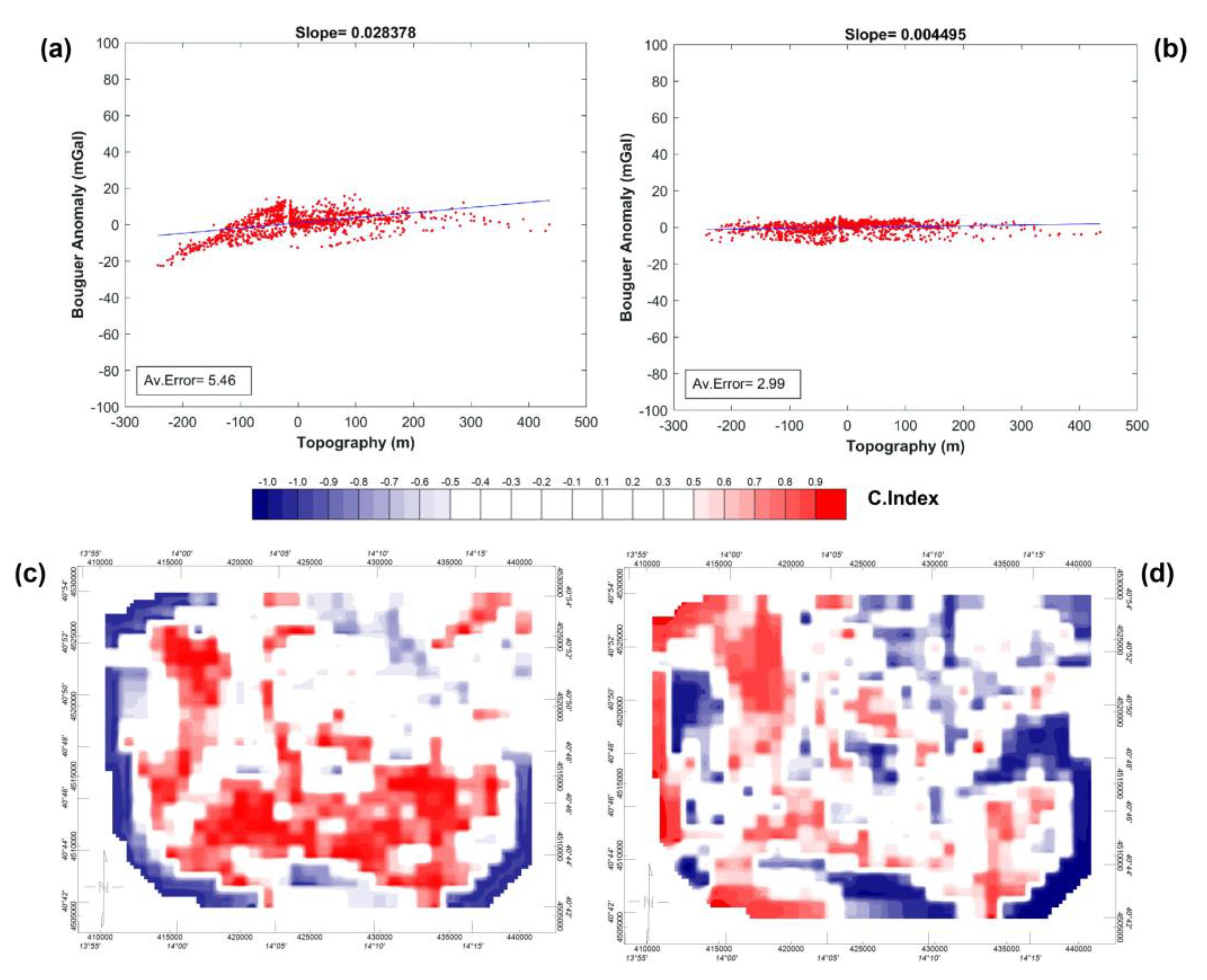
Figure 1. Geo-structural map of the Phlegraean Fields areas. Faults and caldera rims modified by Vitale and Isaia 2014 [22], resurgent dome modified by Steinmann et al. 2016 [23], vents modified by Piochi et al. 2014 [24], fumarole modified by De Bonitatibus et al. 1970 [25]. In the upper right Google Earth inset, the study area.
Remotesensing 15 00209 g001
Figure 2. (a) Regional Digital Elevation Model of the Campanian Plain by EMODnet consortium [30]. (b) High resolution Digital Elevation Model of the Phlegraean Fields caldera by ISMAR−CNR [31].
Remotesensing 15 00209 g002aRemotesensing 15 00209 g002b
Figure 3. Overlay of the CFc VPmg Residual Bouguer anomaly (small box inside the map (a)) onto the regional ISPRA Bouguer map (b). Regional ISPRA Bouguer map displayed on the 3D representation of the Moho depth (km) of the southeastern Tyrrhenian sea as derived by the CRUST1 model [63,64], southern point of view.
Remotesensing 15 00209 g003
Figure 4. CP Eni Free Air anomaly maps and the onshore and offshore CFc gravity stations distribution in the inset (a). CFc Eni Free Air anomaly map (b). Phlegraean Fields TGE as derived by VPmg forward modelling. See text for explanation (c).
Remotesensing 15 00209 g004
Figure 5. Orthogonal 3D cross sections of the two nested CFc and CP topographic models used for the VPmg TGE computation with the regional DEM in transparency (a). Extension of the regional and local area onto the DEM (b). Magnification of the local topographic model observed from the SW point of view (Vertical exaggeration is four times). The three volume units of the VPmg model with their prisms are clearly represented (c). Schematic draw of the standard block mesh vs. the adaptive VPmg mesh. It is possible to observe the different behavior of the prisms at the air/crust and water/crust boundaries (d).
Remotesensing 15 00209 g005
Figure 6. The CBA (a) and the regional de-trended CBA (b) maps of the Phlegraean Fields.
Remotesensing 15 00209 g006
Figure 7. Scatter plots of the CBA vs. topography elevation (a) and regional de-trended CBA field vs. topography elevation. (b). Distribution of the correlation coefficients of the CBA field vs. topography elevations (c) and of the regional de-trended CBA field vs. topography elevations (d). See text for explanation.
Remotesensing 15 00209 g007
Figure 8. VPmg Residual Complete Bouguer anomaly map after removing the regional component; interpreted anomalies and their alignments are labelled with progressive number respectively (H-gravimetric high, L-gravimetric low and Lnt linear clustering of features) (a). Residual Complete Bouguer anomaly overlaid on the Digital Elevation Model, the figure shows the name of the main localities together with the inner (Yellow Tuff in dashed black lines) and the outer (Ignimbrite Campana in dashed black half thick right lines) caldera rims as derived by Vitale and Isaia [22]. The faults displayed in Figure 1 are also reported in dashed white lines (b).
Remotesensing 15 00209 g008
Table 1. Correlation coefficients.
Bouguer Reduction
Methods
Correlation
Coefficient
Vpmg−0.4107
Residual Vpmg0.1471
Disclaimer/Publisher’s Note: The statements, opinions and data contained in all publications are solely those of the individual author(s) and contributor(s) and not of MDPI and/or the editor(s). MDPI and/or the editor(s) disclaim responsibility for any injury to people or property resulting from any ideas, methods, instructions or products referred to in the content.

