Corrections of Mesoscale Eddies and Kuroshio Extension Surface Velocities Derived from Satellite Altimeters

Abstract

Oceanic datasets derived from satellite altimeters are of great significance to physical oceanography and ocean dynamics research and the protection of marine environmental resources. Ageostrophic velocity induced by centrifugal force is not considered in altimeter products. This study introduces an iterative method to perform cyclogeostrophic corrections of mesoscale eddies’ surface velocities derived from satellite altimeters. The corrected eddy velocity field and geostrophic velocity field were compared by combining eddy detection and mathematical statistics methods. The results show that eddies with small curvature radii, high roundness, or Rossby number larger than 0.1 illustrate that cyclogeostrophic correction is required. The cyclogeostrophic velocity is greater (less) than the geostrophic velocity in anticyclonic (cyclonic) eddies. Additionally, the iterative method is applied to cyclogeostrophic-corrected multi-year (1998–2012) Kuroshio surface velocities. The effect of cyclogeostrophic correction is significant for the Kuroshio Extension region, where the maximum relative difference of velocities with and without correction is about 10% and the eddy kinetic energy is 20%.

1. Introduction

Satellite altimeters are important marine microwave remote sensors where measured data can be applied to physical oceanography, marine dynamics, marine climates and environments, and sea ice monitoring. For example, the distribution characteristics of regional- and global-scale surface current fields [1], the variation characteristics of mesoscale ocean circulation [2,3] and western boundary currents (such as the Kuroshio and the Gulf Stream) [4,5], the dynamic fluctuation of the sea surface [6], the ocean tidal wave system [7], the propagation of sea surface gravity waves [8], and the role of ocean dynamic phenomena in global climate change and El Niño–Southern Oscillation [9]. Based on the linear relationship between the sea surface pressure gradient force and the sea surface current field, quasi-steady sea surface velocities are derived from altimeters without considering the effect of the sea surface wind stress [10,11,12,13,14,15]. However, the classical geostrophic balance theory ignores the centrifugal force acting on the actual current when it moves along a curved path, which results in biases in the sea surface velocity derived from altimeters under the geostrophic balance assumption [16,17,18,19,20]. This bias is different from the ageostrophic velocity component caused by the sea surface wind stress, and it is mainly caused by the nonlinear term induced by the local curvature of the streamline.

Douglas and Richman [20] compared the azimuthal velocities of some intense mesoscale eddies in the Gulf Stream using altimeter and numerical model data. They proposed that a more complete statistical description, including nonlinear terms, can be obtained from observation data by properly considering the dynamics of eddies. Uchida et al. [16] corrected the sea surface velocity derived from satellite altimeters by taking into account the ageostrophic component caused by the curvature of the Kuroshio. The curvature effect of streamlines corrects the geostrophic balance between the pressure gradient force and Coriolis force to the balance between pressure, Coriolis and centrifugal forces (Figure 1). This balanced state is called “cyclogeostrophic balance,” and the current under this balance is called a “cyclogeostrophic current” [21]. A cyclogeostrophic current is a kind of approximate geostrophic current, which is the correction of centrifugal acceleration to the current along the curved streamline. This correction is very important in strong eddies and eddies with Rossby numbers (Ro) close to 1. Small Ro numbers indicate that the motion is significantly affected by Coriolis force, while large Ro numbers indicate that the motion is dominated by inertial force (centrifugal force) [11].

With the development of the new generation of high-resolution marine remote sensing satellites, ocean current curvature-induced biases can no longer be ignored. Penven et al. [19] corrected the geostrophic velocity derived from the altimeter and accurately evaluated the current field, especially the azimuth velocity of the anticyclonic eddies in the Mozambique Strait. Ioannou et al. [22] cyclostrophically corrected the surface geostrophic velocity derived from altimeters for eddies with strong ageostrophic components in the Mediterranean Sea. While several studies focused on the correction of mesoscale eddies surface velocity derived from altimeters, little is known about the correction methods and dynamic characteristics of eddies with different shapes and sizes as well as meanders.

In this paper, based on satellite altimeter data, the surface velocities of mesoscale eddies and Kuroshio are cyclogeostrophically corrected by an iterative method, and the dynamic characteristics of the cyclogeostrophic current field are discussed. Section 2 provides a description of the materials and methods used in this study. The main results are given in Section 3. The influence mechanism of cyclogeostrophic correction is discussed in Section 4, and the summary is presented in Section 5.

2. Data and Methods

2.1. Satellite Altimeter Data

This study uses the gridded-merged sea surface height (SSH) satellite altimeter data provided by Validation and Interpolation of Satellite Oceanographic (AVISO). AVISO altimetry gridded data are produced by merging multi-satellite altimeters (European remote sensing satellite, TOPEX/Poseidon, Jason-1, Jason-2, Cryosat2, SARAL/ALtiKa, and HY-2) and the data unification and altimeter combination system (DUACS) [23]. The geostrophic velocities used in this study are derived from the absolute dynamical topography provided by AVISO.

The daily AVISO/DUACS DT2018 data have a spatial resolution of 1/4° and extend from January 1998 to December 2012. The mesoscale errors of the DT2018 data are estimated using independent and in situ measurements. Due to the influence of various disturbances (e.g., atmosphere and instruments) on the altimeter, DT2018 adopts dynamic atmospheric correction (DAC) and ocean tide correction. Additionally, DT2018 uses new altimetry standards and geophysical corrections, improves data selection, and applies optimum interpolation (OI) parameters for global and regional map generation. Compared with the previous version, the geostrophic currents error of DT2018 has been reduced by about 5% globally [23].

2.2. Methods

2.2.1. Skewness

Skewness is a measure of the degree of asymmetry of statistical data distribution relative to the mean [24]. For a sample of n values, the skewness (sk) is calculated as follows:

$$\begin{array}{l}sk=\frac{n{\displaystyle \sum {\left(x_i-\overline{x}\right)}^3}}{\left(n-1\right)\left(n-2\right)s^3}\begin{array}{cc}& \end{array}\\ s=\sqrt{\frac{1}{n-1}{\displaystyle \sum {\left(x_i-\overline{x}\right)}^2}}\\ \Rightarrow sk=\frac{n{\displaystyle \sum {\left(x_i-\overline{x}\right)}^3}}{\left(n-1\right)\left(n-2\right){\left(\frac{1}{n-1}{\displaystyle \sum {\left(x_i-\overline{x}\right)}^2}\right)}^{\frac{3}{2}}}\end{array},$$

(1)

where s is the standard deviation of the data, $\overline{x}$ is the mean of the data, and x_i is the i-th of the data sample. Skewness is defined by using the third moment. For a group of asymmetric data, a positive (sk > 0) means that the data with smaller relative average values are relatively centralized, while a negative (sk < 0) means that the data with larger relative average values are relatively centralized. The skewness of normal distribution sk = 0.

2.2.2. Iterative Algorithm

Many nonlinear equations of ocean dynamics cannot be solved analytically. In most cases, the approximate solution of nonlinear equations can only be obtained by numerical calculations. An iterative algorithm is a common method in numerical analysis. The iterative algorithm uses an initial value to generate a sequence of improving approximate solutions for a class of problems in which the n-th solution is the best approximation of the solution [25,26,27]. Iteration can be divided into precise iteration and approximate iteration. The most common methods, the Newton iteration method [28] and bisection method [29], are approximate iteration methods. The iterative method consists of three steps:

• Determine the initial value;
• Derive the iteration equation;
• Determine the conditions for the termination of the iterative sequence.

The iterative method is a process of taking a limit, which requires multiple iterations. Only convergent iterations have practical significance. For multivariate nonlinear equations (e.g., vectors and matrices), the concept of the norm can be introduced to judge whether the iterative method converges. The norm can be estimated as follows:

$$\left|\right|\overrightarrow{X}-\overrightarrow{Y}\left|\right|=\sqrt{{(x_2-x_1)}^2+{(y_2-y_1)}^2},$$

(2)

where $\overrightarrow{X}(x_1,y_1)$ and $\overrightarrow{Y}(x_2,y_2)$ are two vectors. Common criteria for stopping the iteration are (a) when the change of the independent variable is sufficiently small, i.e., $\Vert {\overrightarrow{x}}^{(k+1)}-{\overrightarrow{x}}^{(k)}\Vert <\epsilon$ ($\epsilon$ is a small value) and (b) when the function value drops sufficiently.

Penven et al. [19] used an iterative method to solve the equation of sea surface cyclogeostrophic current:

$${\overrightarrow{U}}^{\left(n+1\right)}-\frac{\overrightarrow{k}}{f}\times \left({\overrightarrow{U}}^{\left(n\right)}\cdot \nabla {\overrightarrow{U}}^{(n)}\right)={\overrightarrow{U}}_g,$$

(3)

where $f=2\Omega \sin \varphi$ is the Coriolis parameter, $\Omega$ is the angular frequency of the rotation of the Earth, $\varphi$ is the latitude, $\overrightarrow{k}$ is the vertical unit vector, $\overrightarrow{U}$ is the velocity vector of sea surface horizontal current, ${\overrightarrow{U}}_g$ is the velocity vector of the sea surface geostrophic current, and n is the number of iteration steps. The norm calculation equation of the iterative algorithm [Equation (3)] is as follows:

$$\Vert {\overrightarrow{U}}^2(u^2,v^2)-{\overrightarrow{U}}^1(u^1,v^1)\Vert =\sqrt{{\left(u^2-u^1\right)}^2+{\left(v^2-v^1\right)}^2},$$

(4)

where u is the zonal velocity and v is the meridional velocity. This iterative algorithm may diverge after a few steps [19]. According to Penven et al. [19] and Ioannou et al. [22], for intense mesoscale eddies, the iteration occurs for each grid point, and the criterion for stopping iteration is when $\epsilon$ is 0.01.

For meanders, in order to determine the convergence scheme of the iterative algorithm, this study tests the velocity of a curved section of meander located in the Kuroshio derived by satellite altimeter on 12 August 1998. First, the local norm $\epsilon$ is set as 0.01 and calculated on the central grid point and the eight nearest grid points. Second, the velocities in the curved jet section, which are located on the grid point with longitude 145.375°E and latitudes 32.125°N to 35.875°N (blue dotted line in Figure 2) are corrected using the iterative algorithm. The maximum and minimum velocity of grid points selected for testing is 1.2 and 0.1 m/s, respectively. The convergence is slower after five steps [22]. When the initial geostrophic speed is large, the scheme converges quickly after four iterations, as shown in Figure 3. Figure 3a shows that the norm value of the tested points with large velocity is generally less than 0.01 after the third iteration, the norm value of the points with small velocity is less than 0.01 after the first iteration, and the norm value of some points is less than 0.01 in the first iteration. Comparing the geostrophic velocity with the velocity after each iteration (Figure 3b), it is found that the cyclogeostrophic correction of the velocity at grid points with large velocity or large curvature is significant, and the cyclogeostrophic velocity is greater than the geostrophic velocity. Combined with the variation characteristics of velocity and norm, the grid resolution of the altimeter merged data is 1/4° × 1/4°. To ensure the accuracy of the correction, the judgment condition of convergence is determined as stop iterative calculation when the local norm value is less than 0.01 or starts to increase. In addition, it should be noted that for grid points with small geostrophic velocities, the number of iteration steps is only one.

In order to evaluate the effects of the cyclogeostrophic correction, the relative difference of average velocity (a_v) can be defined as:

$$a_v=\left({\displaystyle {\sum }_j^n{S}_{(la{t}_{j}lo{n}_j)}\times \left[(V_i-V_g)/V_g\right]\times 100\%}\right)/{\displaystyle {\sum }_j^n{S}_{(la{t}_{j}lo{n}_j)}},$$

(5)

where V_i is the cyclogeostrophic velocity, V_g is the geostrophic velocity, and S_(lati,loni) is the grid area.

2.2.3. Eddy Automated Detection Algorithm

Eddies can be defined as a region where the velocity vector rotates clockwise or anticlockwise around a central point. Automated eddy detection technology can be classified by those that use either Eulerian or Lagrangian data. Based on the Eulerian method, eddies can be detected by two- or three-dimensional field images (snapshot data at a certain time). In contrast, the Lagrangian method can be used to identify eddies by tracking particles. In this study, a Eulerian eddy-detection algorithm is used to identify eddies [30]. The algorithm has been successfully applied to eddy detection in the global oceans [31]. The algorithm is as follows. The center of the eddy is determined by the geometry of the velocity vector through four limiting conditions [32,33,34]:

• In the east–west direction along the eddy center, the v’ component of velocity has opposite signs on both sides of the eddy center, which gradually increases away from the center point;
• In the north–south direction along the eddy center, the u’ component of velocity has opposite signs on both sides of the eddy center, which gradually increases away from the center point;
• In the local region of the eddy center, the velocity is the minimum;
• Around the eddy center, the rotation of the eddy velocity vector is consistent. The direction of two neighboring velocity vectors must be in the same or two neighboring quadrants.

Here u’ and v’ are the surface velocity anomalies of zonal and meridional currents. The minimum velocity detected by the first three limiting conditions is not necessarily related to the eddy structure and cannot be directly defined as the eddy center. Therefore, the fourth limiting condition must be introduced to prevent false detection. The fourth limiting condition can successfully distinguish the local velocity minima related to eddies and avoid excessive detection of eddies. The grid point satisfied by the above four conditions is identified as the eddy center. Once the eddy center is determined, the boundaries of each eddy can be calculated. The eddy boundary is defined by the contour of stream function. The eddy velocity field is weak divergence, and the velocity vector is tangent to the stream function contour. With the increase of the tangential velocity, the tangential velocity reduces at the eddy boundary. Therefore, the boundary of the eddy is defined as the outermost closed contour around the center point.

2.2.4. Rossby Number

The eddy Rossby number, which is related to the maximum eddy radius (R_max) and velocity (V_max), is calculated by:

$$Ro=\frac{V_{\max }}{f{R}_{\max }},$$

(6)

The normalized relative eddy vorticity used to characterize the motion state of the eddy can be estimated as follows:

$$\frac{\zeta }{f}=\frac{\partial v^{\prime }/\partial x-\partial u^{\prime }/\partial y}{f}~Ro,$$

(7)

where $\zeta$ is the relative vorticity.

The cyclogeostrophic Rossby number (CRo) is given by [21]:

$$CRo=\frac{v_i{}^2}{f{r}_0},$$

(8)

where r₀ is the radius of curvature. If the current moves along a straight path (i.e., r₀ tends to infinity), then CRo tends to 0 ($v=v_g$). If $CRo\ne 0$ ($v\ne v_g$), then the current flow path must be curved. For different latitudes, speeds, and shapes of currents, the sensitivity of r₀ to the dynamic process of cyclogeostrophic current is different. Assuming that the radius of curvature is the same (r₀ = R, where R is a constant), the CRo is related to the cyclogeostrophic velocity and the Coriolis parameter.

2.2.5. Eddy Kinetic Energy

Eddy kinetic energy (EKE) is a very important energy in the ocean which can be calculated by the geostrophic current velocity estimated using altimeters. EKE can be estimated by:

$$EKE=\frac{1}{2}\times \left[{\left(u^{\prime }\right)}^2+{\left(v^{\prime }\right)}^2\right],$$

(9)

The relative difference in EKE (a_eke) is

$$a_{eke}=\left[\left(EK{E}_i-EK{E}_g\right)/EK{E}_g\right]\times 100\%,$$

(10)

where EKE_i and EKE_g are the eddy kinetic energy of the cyclogeostrophic and geostrophic eddies, respectively.

3. Results

This section mainly uses the iterative algorithm to correct the geostrophic current derived from altimeter data. The differences of the kinematic characteristics between the cyclogeostrophic and geostrophic current in eddies are investigated in Section 3.1. The differences between the cyclogeostrophic current and the geostrophic current in the Kuroshio Extension region are statistically analyzed in Section 3.2.

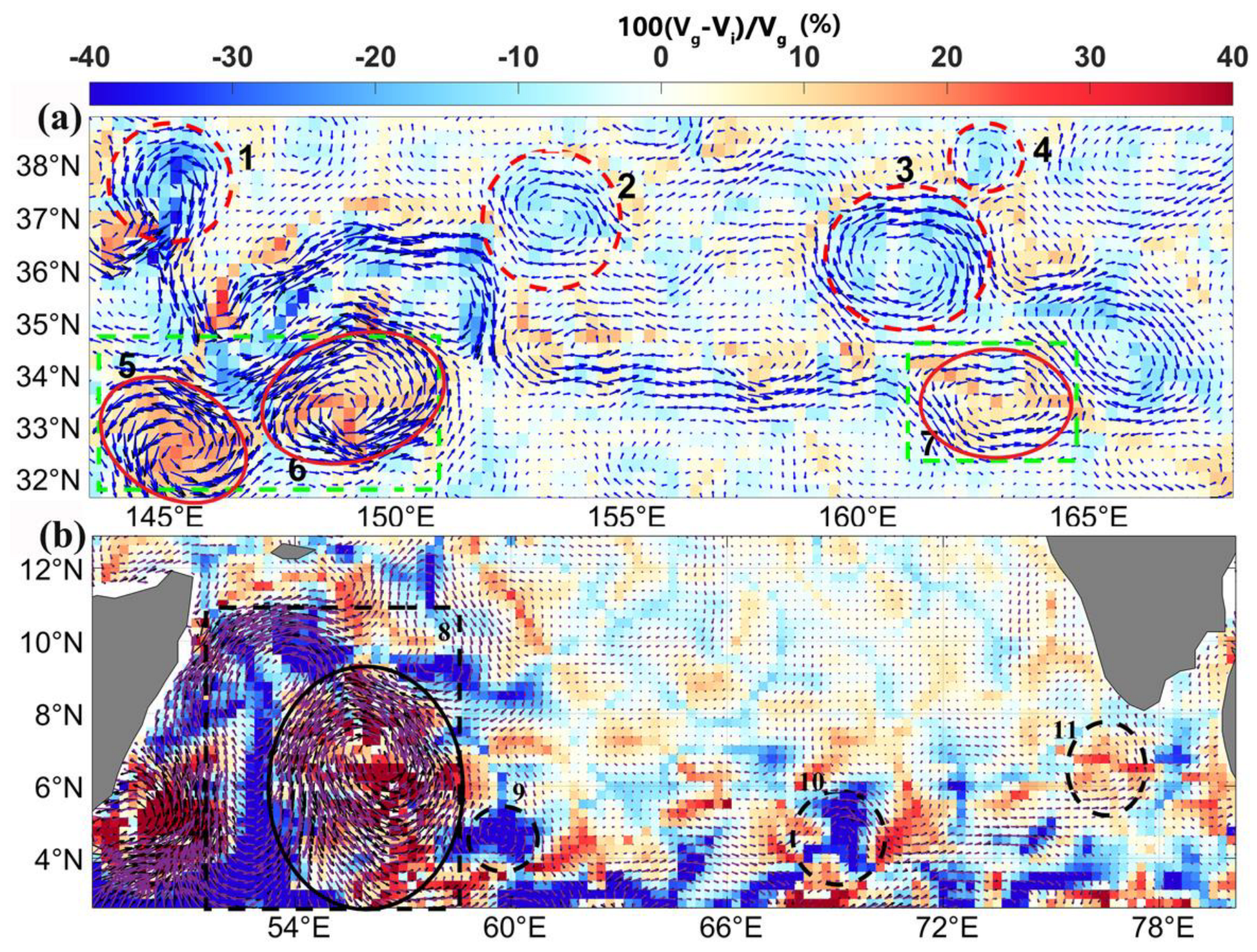
3.1. Cyclogeostrophic Corrected Surface Velocities of Eddy

Eddies are among the most common dynamic processes in global ocean circulation. According to their rotational characteristics, they can be divided into cyclonic and anticyclonic eddies. Due to their different rotation directions, their kinematics and dynamics characteristics are also different. Therefore, it is necessary to discuss the cyclonic eddy and anticyclonic eddy separately when studying the influence of the cyclogeostrophic correction. In order to quantitatively analyze the influence of cyclogeostrophic correction on the difference in eddy kinematics, ten eddies were randomly selected: five cyclonic and five anticyclonic eddies.

Table 1. Comparison of the cyclogeostrophic and geostrophic currents of ten eddies in the Northern Hemisphere on 12 August 1998.

Case	Type	Vgmax (m/s)	Vimax (m/s)	Lat (°N)	Rog	Roi	av (%)
Case 1	CE 1	1.36	1.11	30–31	0.30	0.25	−14.34
Case 2	CE	1.13	1.08	32–34	0.08	0.07	−7.90
Case 3	CE	1.24	1.20	35–36	0.23	0.22	−11.95
Case 4	CE	1.17	1.06	34–35	0.18	0.17	−10.31
Case 5	CE	1.33	1.19	36–37	0.21	0.19	−11.09
Case 6	ACE 2	1.05	1.14	36–38	0.12	0.13	8.69
Case 7	ACE	1.25	1.36	39–41	0.07	0.08	8.81
Case 8	ACE	0.85	0.86	40–42	0.08	0.09	8.92
Case 9	ACE	0.14	0.16	7–8	0.11	0.12	8.94
Case 10	ACE	0.41	0.52	8–9	0.23	0.29	17.22

¹ Cyclonic eddy (CE). ² Anticyclonic eddy (ACE).

displays the maximum geostrophic velocity (V_gmax), the maximum cyclogeostrophic velocity (V_imax), the geostrophic vortex Rossby number (Ro_g), the cyclogeostrophic vortex Rossby number (Ro_i), and a_v.

The five cyclonic eddies are located in mid-latitudes. In Case 1, the cyclonic eddy intensity is the largest: V_gmax reaches 1.36 m/s, Ro_g is 0.3, the maximum velocity is 1.11 m/s after cyclogeostrophic correction, Ro_i is 0.25, and the difference ratio of the weighted average velocity of the eddy is −14.34%. The cyclogeostrophic correction of this eddy is the most significant among the five cyclonic eddies. The velocity of the eddy is the smallest in Case 2, and the Ro_g is only 0.08, the a_v is only −7.90%, which is the smallest correction effect among the ten cases. The result shows that the smaller the Ro_g is, the weaker the influence of centrifugal force on the eddy. As a result, the difference between the geostrophic and circyclogeostrophic velocity of this eddy is small. Comparing a cyclonic eddy (Case 2) with an anticyclonic eddy (Case 8), it is found that when the Ro_g is the same, the correction of the anticyclonic eddy is more important than that of the cyclonic eddy. The anticyclonic eddy of Case 10 is located in the low latitude seas, where the Coriolis parameter is relatively small, and V_gmax is also small (0.41 m/s). However, its Ro_g is 0.23, and the a_v is 17.22%. The cyclogeostrophic correction is important for this eddy. A comprehensive analysis of the parameters of the ten eddies shows that the larger the Ro_g, the greater the absolute value of a_v, and the more important the cyclogeostrophic correction. In summary, the cyclogeostrophic correction is significant for eddies with Ro_g greater than 0.1 [22]. The cyclogeostrophic velocities of the cyclonic eddies are lower than the geostrophic velocities, and the cyclogeostrophic velocities of the anticyclonic eddies are higher than the geostrophic velocities.

In order to more specifically analyze the difference in the kinematic and dynamic characteristics of the eddies under geostrophic balance and cyclogeostrophic balance, this paper analyzes the spatial distribution characteristics of the velocity, eddy kinetic energy, and relative vorticity of an isolated cyclonic and anticyclonic eddy. Figure 4 shows a cyclonic eddy in the Southern Hemisphere. Comparing the cyclogeostrophic velocity with the initial geostrophic velocity, it is found that the geostrophic velocity of a cyclonic eddy is greater than the cyclogeostrophic velocity, with a maximum difference ratio of 30% (Figure 4a). For a region with large streamline curvature, the difference between the cyclogeostrophic and the geostrophic current directions are large. In addition, the spatial distribution characteristics of the percentage difference of EKE of the two current fields are shown in Figure 4b. The results show that the EKE under geostrophic equilibrium overestimates the actual EKE, and the maximum a_eke can reach 40%, which is consistent with the conclusions of Maximenko and Niiler [35]. The eddy detection method is used to detect the initial geostrophic and cyclogeostrophic current fields. It is found that the position of the corrected eddy center has not changed, but the boundary shape of the cyclonic eddy is slightly different. The corrected eddy boundary is smaller than the boundary of the initial geostrophic eddy. The Rossby number quantifies the relative importance of centrifugal force and Coriolis force. In order to study the influence of centrifugal force on the eddy, the normalized relative vorticity (Figure 4c) of the eddy is more suitable for studying the importance of centrifugal force in a regional current field. The normalized relative vorticity of the cyclonic eddy under geostrophic balance reaches 0.6 at the eddy center, indicating that the centrifugal force compared with the Coriolis force on the eddy is not negligible. Figure 4d shows the relative vorticity of the cyclogeostrophic current, which is weaker than the initial geostrophic current, and its polarity has not changed.

The thermodynamic, kinematic, and dynamic characteristics of anticyclone eddies in the ocean are significantly different from those of cyclonic eddies. Therefore, this study selected an anticyclone eddy in the northern hemisphere for discussion. Calculating the percentage difference between the corrected cyclogeostrophic velocity and the initial geostrophic velocity (Figure 5a) shows that the velocity based on the altimeter underestimates the actual eddy velocity. The difference in corrected eddy velocity is about 50%, and the direction of current changes significantly at the grids near the eddy center. Figure 5b shows the relative difference in EKE. It is found that the difference of EKE is obvious, and the maximum a_eke exceeds 85%. The boundary of the cyclogeostrophic eddy is larger than the initial geostrophic eddy detected by the eddy detection method. The geostrophic relative vorticity at the eddy center is 0.4 (Figure 5c), and the cyclogeostrophic relative vorticity increases to 0.6 (Figure 5d).

According to the difference analysis of the kinematic characteristics of the above two eddies, the correction has a certain impact on the shape of the eddy. Eight eddies with different shapes were randomly selected (four cyclones and four anticyclones), as shown in Figure 6. For the elliptical eddy, the effect of cyclogeostrophic correction on the eddy boundary was not significant (Figure 6b–d,f). For the eddy with high roundness, the cyclogeostrophic correction had a significant effect on the eddy boundary (Figure 6a,e,g).

Comparing the distribution characteristics before and after the cyclogeostrophic correction shows that the cyclogeostrophic correction had a significant impact on the eddy dynamic process, especially for the eddy whose Ro_g was greater than 0.1 and EKE difference was large. Second, the effect of the correction on the anticyclonic eddy was greater than that on the cyclonic eddy. In addition, the shape of the eddy with high roundness was noticeably changed by the corrections.

3.2. Cyclogeostrophic Corrected Surface Velocities of Kuroshio Extension

Western boundary currents are warm, deep, narrow ocean currents and jets formed on the western side of a given ocean basin and continental slope due to western intensification. They transport warm water from the tropics to the poles. Relevant to the current study, the Kuroshio in the Pacific Ocean originates in the southeast of the Philippines coast, flowing northward along the east coast of Taiwan Island and the continental slope in the East China Sea [36]. Many studies compared the surface velocity from satellite altimeter and drift buoy data in the Kuroshio current and found that there were differences between the two observational platforms [16,18,37,38]. The non-geostrophic velocity component caused by sea surface wind stress is one of the reasons for the difference [18]. The Kuroshio has a large meandering structure free from topographic constraints, and the two sides of the main axis are full of curved currents of various scales [39,40,41]. By distinguishing the non-geostrophic velocity caused by surface wind stress, Uchida et al. [16] pointed out that the curvature of the Kuroshio increased the small non-geostrophic velocity component and improved the surface velocity calculated by satellite altimetry (TOPEX/POSEIDON). Therefore, it is of great scientific significance to study the cyclogeostrophic velocities of the Kuroshio. The iterative algorithm in Section 2.2.2 is applied to the Kuroshio Current system based on altimeter data gridded at 1/4° resolution from 1998–2012.

Figure 7 analyzes the distribution characteristics of the cyclogeostrophic velocities and the spatial difference between the cyclogeostrophic and the initial geostrophic velocities in the Kuroshio Current system. The large multi-year average cyclogeostrophic velocities are distributed in the Kuroshio Extension region (Figure 7a). Figure 7b shows the spatial difference between the multi-year average velocity of the cyclogeostrophic current and the geostrophic current. It was found that cases in which the cyclogeostrophic velocity was less disturbed than the geostrophic velocity were mostly distributed in the south of the Kuroshio Extension path, and cases in which the cyclogeostrophic velocity was greater than the geostrophic velocity were mostly distributed in the north of the Kuroshio Extension path. The maximum relative difference is 10%. Additionally, for grid points with small geostrophic velocities, there are differences between the cyclogeostrophic and the geostrophic velocities with a relative difference of about 2%.

According to the EKE statistical analysis, the maximum cyclogeostrophic average EKE is above 1500 cm²/s² in the Kuroshio Extension region (Figure 8a). For the quantitative analysis of the difference between the cyclogeostrophic and the geostrophic average EKE, the spatial difference characteristics are shown in Figure 8b. The spatial characteristics of the EKE difference are similar to those of the velocity difference. The positive difference is distributed north of the Kuroshio Extension path, and the negative difference is to the south. The relative difference in EKE is much greater than that of velocity, with a maximum relative difference of about 20%. The relative difference for grid points with small velocity is about 5%.

By correcting the Kuroshio Current velocities derived from altimeters, the difference between the corrected and geostrophic current fields can be analyzed. The results show that the correction has a significant impact on the change in EKE. The difference between the cyclogeostrophic current and the initial surface current derived from altimeters on both sides of the Kuroshio main axis is bipolar. Figure 9 shows the skewness distribution (1998–2012) of the sea surface height anomaly (SSHA) in the Kuroshio Extension region. The spatial pattern resembles the difference of velocity and EKE between cyclogeostrophic current and initial surface current, in which the positive SSHA are more probable than negative ones north of the Kuroshio Extension axis and the negative SSHA are more probable than positive ones south of the Kuroshio Extension axis. The dynamic structure of ocean eddies and jets may be the reason for the skewness distribution of SSHA [35]. The movement of an eddy causes local convergence and divergence of sea water. Ji et al. [32] pointed out that in the Kuroshio Extension, eddies are generated by the unstable meandering path. According to this eddy generation mechanism, more cyclonic (anticyclonic) eddies with long lifespans are in the south (north) of 35°N. The cyclonic eddy presents a negative SSHA, in which the central sea surface height is lower than the surrounding region. The SSHA of the anticyclonic eddy is positive, meaning that its center is higher than the surrounding region [42].

4. Discussion

The effects of centrifugal forces are important in curved currents [19,21]. The correction of geostrophic currents derived from altimeters is of great significance. Thus, mesoscale currents at the sea surface need to be further evaluated. A discussion of the influence mechanism of cyclogeostrophic correction can deepen our understanding of mesoscale eddies’ and meanders’ dynamics.

4.1. Interpretation of the Cyclogeostrophic Rossby Number

Eleven eddies were selected to evaluate the role of cyclogeostrophic Rossby number based on Equation (8) (Figure 10). Detailed information on the eddies is listed in

Table 2. Information on the eleven selected eddies.

No.	Vimax (m/s)	f (s−1)	Radius (km)
1	1.2	8.9 × 10−5	110
2	0.7	8.7 × 10−5	125
3	1.0	8.6 × 10−5	150
4	0.4	9.0 × 10−5	50
5	1.4	7.9 × 10−5	100
6	1.4	8.0 × 10−5	150
7	0.8	8.0 × 10−5	125
8	2.0	1.8 × 10−5	300
9	0.6	1.2 × 10−5	50
10	0.8	1.2 × 10−5	75
11	0.4	1.6 × 10−5	75

. The curvature radius and velocity of eddy No. 6 in Figure 10a and eddy No. 8 in Figure 10b are similar, but the Coriolis parameter of eddy No. 8 (located in low latitudes) is about 1.8 × 10⁻⁵ and that of eddy No. 6 is about 8 × 10⁻⁵. Notably, the CRo of No. 8 is greater than that of eddy No. 6. The correction of eddy No. 8 has a significant impact on the relative difference of velocity. In the mid-latitudes (with similar Coriolis parameters), cyclonic eddy No. 6 and anticyclonic eddy No. 3 have similar radii, but the two eddies have different velocities. The velocity of eddy No. 6 is larger than that of eddy No. 3, leading to different cyclogeostrophic correction effects. Eddies No. 1 and No. 4 at the same latitude, the curvature radius of eddy No. 1 is larger than No. 4, the correction of eddy No. 1 has more significant impact on the relative difference of velocity. The Coriolis parameters are similar for eddies No. 5, No. 6, and No. 7 at the same latitude, and the first two eddies have larger velocities. Figure 10a shows that the effects of the cyclogeostrophic correction on the speed of eddy No. 5 and No. 6 are significantly greater than that of No. 7. The same result is also shown in the comparison between eddies No. 2 and No. 3. The maximum velocities of eddy No. 5 and No. 6 are the same, but the curvature radius of eddy No. 5 is smaller than that of eddy No. 6, such that the CRo of eddy No. 5 is larger, and the influence of the cyclogeostrophic correction of eddy No. 5 on the relative difference of velocity is significant (Figure 10a). Similarly, for eddies No. 9 and No. 10 at low latitude, the curvature radius of eddy No. 9 is smaller than that of eddy No. 10, and the relative difference in velocity is also significantly greater than that of eddy No. 10 (Figure 10b).

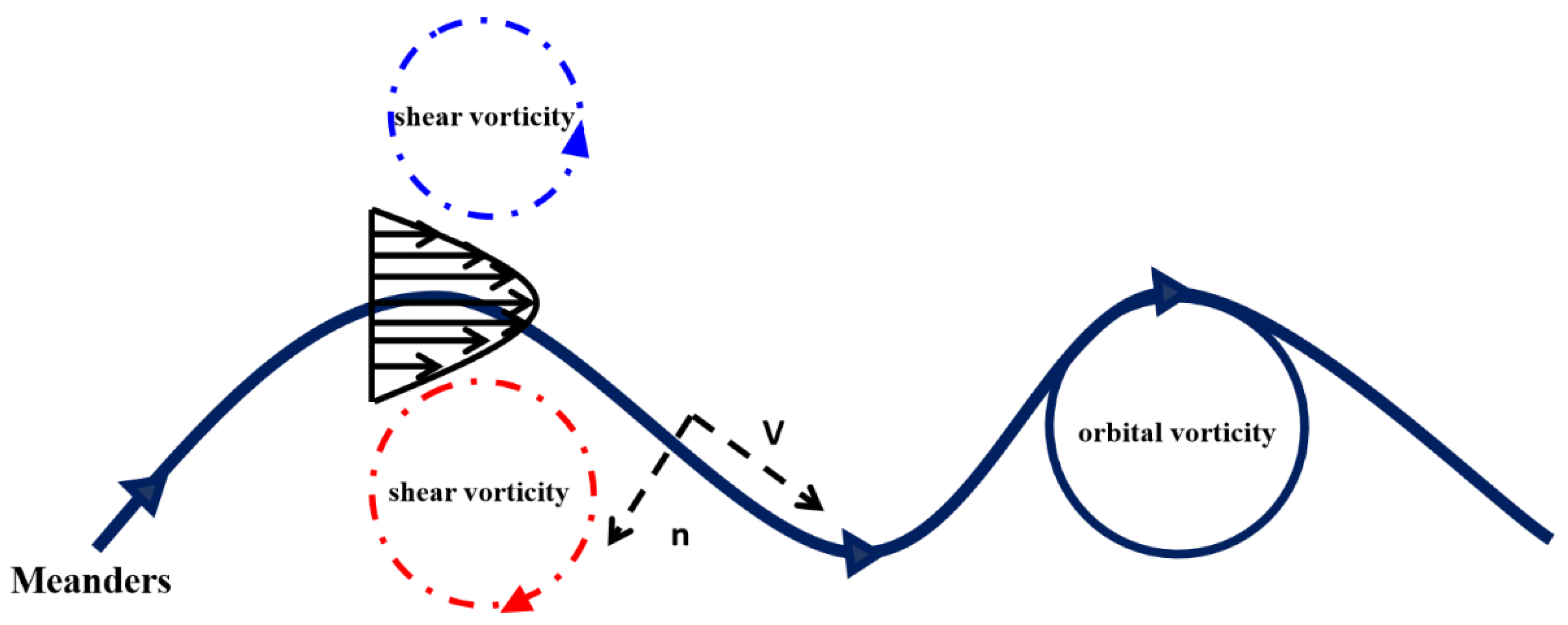
4.2. Vorticity Adjustment of Meander

According to the results in Figure 9 and the generation mechanism of eddies in the Kuroshio Extension region, the difference in the cyclogeostrophic correction may be related to the relative vorticity of the sea surface current. Neglecting the β-effect and the vertical stretching and extrusion, the relative vorticity is conserved [43]:

$$\zeta =\frac{\partial v}{\partial x}-\frac{\partial u}{\partial y}=\frac{\partial V}{\partial n}-\kappa V,$$

(11)

where $V=\sqrt{u^2+v^2}$ is the velocity in the horizontal direction, and n is the coordinate direction perpendicular to the meander path. In natural coordinates, the relationship between the relative vorticity and curvature of the current is reflected. In Equation (11), $\frac{\partial V}{\partial n}$ is the shear contribution term, which is called “shear vorticity”. $-\kappa V$ is the vorticity generated by turning off the current path, which is called “orbital vorticity”. $\kappa$ is the meander path curvature (the positive values represent the clockwise rotation). In the Northern Hemisphere, when the fluid turns to the right of the meander axis, the fluid particles adopt a clockwise orbital vorticity of magnitude $\kappa V$. Due to the conservation of relative vorticity, it must be related to the shear vorticity $\frac{\Delta U}{L}$ (Figure 11). The adjustment of shear vorticity means that the fluid particle tends to move towards the meander path. Specifically, the fluid particle has the maximum velocity upstream of the meander (main axis), without shear and orbital vorticity. If the particle turns right in the meander, it gains clockwise orbital vorticity, which must be compensated by a counterclockwise shear vorticity of the same order. At the same time, the particle must be located on the left side of the meander. The adjustment of orbital vorticity means that the movement of the meander changes, or the fluid particle tends to leave the meander path. The fluid particle occupying the main axis (with maximum velocity and no shear vorticity) is located on the right side of the upstream of the meander, and its entire clockwise shear vorticity is converted into an equivalent clockwise orbital vorticity [43]. It can be concluded that all of the fluid particles tend to move to the left relative to the main axis at the right turn and to the right relative to the main axis at the left turn. That is, fluid particles move in the direction of centrifugal force in the meander. The vorticity adjustment required by the meander may change the direction of rotation of the fluid particle at the edge of the main axis, resulting in a mesoscale ring off the main axis.

As one can see from the above, the method proposed in the present study is aimed to improve the accuracy in the extraction of velocity information from satellite altimetry data, which is related to eddies and meanders resolved by the SSH data. The latter strongly dependents on the quality of the interpolation of the along-track satellite altimetry data.

5. Conclusions

This study investigates the corrections of the sea surface velocity field of mesoscale eddies and meanders derived from altimeters based on an iterative method. Iterative experiments are carried out on various shapes of eddies and Kuroshio Current systems in order to determine the iteration algorithm for geostrophic current observed by the altimeters with a grid resolution of 1/4 × 1/4°. For mesoscale eddies, the convergence condition is that the iteration is stopped when the local norm value is less than 0.01 or starts to increase. For mesoscale curved currents, it should be noted that the number of iteration steps for grid points with small geostrophic velocity is only one.

It is necessary to cyclogeostrophically correct the surface current field derived from satellite altimeters. By analyzing the difference, it can be found that the altimeter data overestimate and underestimate the EKEs of cyclonic and anticyclonic eddies, respectively. Cyclogeostrophic correction has a significant impact on the eddies with geostrophic Rossby numbers greater than 0.1. Combined with the eddy detection method, it is found that the correction significantly changes the shape of eddies with higher roundness. The statistical analysis of the Kuroshio Extension current shows that the effect of the cyclogeostrophic correction of the boundary zonal jet, which is not restricted by topography, is significant. This is especially the case in the section with large curvature. Since there are many eddies with long lives and large velocities on both sides of the path, the effect of cyclogeostrophic correction is significant for the western boundary current. The correction difference of the western boundary current is related to the change in its relative vorticity.

For currents of different latitudes, velocities and shapes, the significance of the cyclogeostrophic correction is mainly determined by CRo. The current flows along a straight line, and the cyclogeostrophic velocity is equal to the geostrophic velocity. The current flows along the curved streamline. When the radius of curvature is the same, the error between the cyclogeostrophic velocity and the geostrophic velocity is related to f and v. When the velocity is the same, the smaller the f, the larger the error. At the same latitude, the larger the velocity, the larger the error. At the same velocity, the smaller the radius of curvature, the larger the error.

The sea surface current derived from satellite altimeters with cyclogeostrophic correction can effectively promote the application of satellite altimeters in studying mesoscale and small-scale ocean current dynamics. Although the cyclogeostrophic correction is very important for AVISO altimeters of 1/4 grid resolution [19], it will become more essential when the sub-mesoscale current is observed by higher-resolution altimeters. With the development of remote sensing technology, the spatial resolution of satellite altimeter is gradually improved, and the smaller-scale phenomena of the sea surface are gradually revealed. Therefore, it is necessary to study the cyclogeostrophic correction.

References

1. Dohan, K.; Maximenko, N. Monitoring Ocean Currents with Satellite Sensors. Oceanography 2010, 23, 94–103. [Google Scholar] [CrossRef] [Green Version]
2. Chelton, D.B.; Schlax, M.G.; Samelson, R.M.; De Szoeke, R.A. Global observations of large oceanic eddies. Geophys. Res. Lett. 2007, 34, L15606. [Google Scholar] [CrossRef]
3. Ji, J.; Dong, C.; Zhang, B.; Liu, Y. An oceanic eddy statistical comparison using multiple observational data in the Kuroshio Extension region. Acta Oceanol. Sin. 2017, 36, 1–7. [Google Scholar] [CrossRef]
4. Mendoza, C.; Mancho, A.M.; Rio, M.H. The turnstile mechanism across the Kuroshio current: Analysis of dynamics in altimeter velocity fields. Nonlinear Process. Geophys. 2010, 17, 103–111. [Google Scholar] [CrossRef] [Green Version]
5. Leterme, S.C.; Pingree, R.D. The Gulf Stream, rings and North Atlantic eddy structures from remote sensing (Altimeter and SeaWiFS). J. Mar. Syst. 2008, 69, 177–190. [Google Scholar] [CrossRef]
6. Ichikawa, K.; Imawaki, S. Fluctuation of the sea surface dynamic topography southeast of Japan as estimated from Seasat altimetry data. J. Oceanogr. 1992, 48, 155–177. [Google Scholar] [CrossRef]
7. Woo, H.-J.; Park, K.-A. Estimation of Extreme Significant Wave Height in the Northwest Pacific Using Satellite Altimeter Data Focused on Typhoons (1992–2016). Remote. Sens. 2021, 13, 1063. [Google Scholar] [CrossRef]
8. Cao, Y.; Dong, C.; Young, I.R.; Yang, J. Global Wave Height Slowdown Trend during a Recent Global Warming Slowdown. Remote Sens. 2021, 13, 4096. [Google Scholar] [CrossRef]
9. Hamlington, B.D.; Leben, R.R.; Kim, K.Y.; Nerem, R.S.; Atkinson, L.P.; Thompson, P.R. The effect of the El Niño-Southern Oscillation on US regional and coastal sea level. J. Geophys. Res. Ocean. 2015, 120, 3970–3986. [Google Scholar] [CrossRef] [Green Version]
10. Lukas, R.; Firing, E. The geostrophic balance of the Pacific Equatorial Undercurrent. Deep Sea Research Part A. Oceanogr. Res. Pap. 1984, 31, 61–66. [Google Scholar]
11. Cushman-Roisin, B. Frontal geostrophic dynamics. J. Phys. Oceanogr. 1986, 16, 132–143. [Google Scholar] [CrossRef]
12. Rikiishi, K.; Sasaki, K. Geostrophic balance of the Kuroshio as inferred from surface current and sea level observations. J. Oceanogr. Soc. Jpn. 1988, 44, 305–314. [Google Scholar] [CrossRef]
13. Strub, P.T.; James, C. Altimeter-derived variability of surface velocities in the California Current System: 2. Seasonal circulation and eddy statistics. Deep. Sea Res. Part II Top. Stud. Oceanogr. 2000, 47, 831–870. [Google Scholar] [CrossRef]
14. Shankar, D.; Vinayachandran, P.N.; Unnikrishnan A., S. The monsoon currents in the north Indian Ocean. Prog. Oceanogr. 2002, 52, 63–120. [Google Scholar] [CrossRef]
15. Armitage, T.W.K.; Bacon, S.; Ridout, A.L.; Petty, A.A.; Wolbach, S.; Tsamados, M. Arctic Ocean surface geostrophic circulation 2003–2014. Cryosphere 2017, 11, 1767–1780. [Google Scholar] [CrossRef] [Green Version]
16. Uchida, H.; Imawaki, S.; Hu, J.H. Comparison of Kuroshio surface velocities derived from satellite altimeter and drifting buoy data. J. Oceanogr. 1998, 54, 115–122. [Google Scholar] [CrossRef]
17. Fratantoni, D.M. North Atlantic surface circulation during the 1990's observed with satellite-tracked drifters. J. Geophys. Res. Ocean. 2001, 106, 22067–22093. [Google Scholar] [CrossRef] [Green Version]
18. Uchida, H.; Imawaki, S. Eulerian mean surface velocity field derived by combining drifter and satellite altimeter data. Geophys. Res. Lett. 2003, 30, 1229. [Google Scholar] [CrossRef]
19. Penven, P.; Halo, I.; Pous, S.; Marié, L. Cyclogeostrophic balance in the Mozambique Channel. J. Geophys. Res. Ocean. 2014, 119, 1054–1067. [Google Scholar] [CrossRef] [Green Version]
20. Douglass, E.M.; Richman, J.G. Analysis of ageostrophy in strong surface eddies in the Atlantic Ocean. J. Geophys. Res. Ocean. 2015, 120, 1490–1507. [Google Scholar] [CrossRef]
21. Shakespeare, C.J. Curved density fronts: Cyclogeostrophic adjustment and frontogenesis. J. Phys. Oceanogr. 2016, 46, 3193–3207. [Google Scholar] [CrossRef]
22. Ioannou, A.; Stegner, A.; Tuel, A.; LeVu, B.; Dumas, F.; Speich, S. Cyclostrophic Corrections of AVISO/DUACS Surface Velocities and Its Application to Mesoscale Eddies in the Mediterranean Sea. J. Geophys. Res. Ocean. 2019, 124, 8913–8932. [Google Scholar] [CrossRef] [Green Version]
23. Taburet, G.; Sanchez-Roman, A.; Ballarotta, M.; Pujol, M.-I.; Legeais, J.-F.; Fournier, F.; Faugere, Y.; Dibarboure, G. DUACS DT2018: 25 years of reprocessed sea level altimetry products. Ocean Sci. 2019, 15, 1207–1224. [Google Scholar] [CrossRef] [Green Version]
24. Von Hippel, P.T. Mean, median, and skew: Correcting a textbook rule. J. Stat. Educ. 2005, 13. [Google Scholar] [CrossRef] [Green Version]
25. Ames, W.F. Numerical Methods for Partial Differential Equations; Academic Press: Cambridge, MA, USA, 2014. [Google Scholar]
26. Dubey, V.P.; Kumar, R.; Kumar, D. A reliable treatment of residual power series method for time-fractional Black–Scholes European option pricing equations. Phys. A Stat. Mech. Its Appl. 2019, 533, 122040. [Google Scholar] [CrossRef]
27. Huang, X.; Zhu, Y.; Vafaei, P.; Moradi, Z.; Davoudi, M. An iterative simulation algorithm for large oscillation of the applicable 2D-electrical system on a complex nonlinear substrate. Eng. Comput. 2021, 38, 3137–3149. [Google Scholar] [CrossRef]
28. Bank, R.E.; Rose, D.J. Global approximate Newton methods. Numer. Math. 1981, 37, 279–295. [Google Scholar] [CrossRef]
29. Tanakan, S. A new algorithm of modified bisection method for nonlinear equation. Appl. Math. Sci. 2013, 7, 6107–6114. [Google Scholar] [CrossRef]
30. Nencioli, F.; Dong, C.; Dickey, T.; Washburn, L.; McWilliams, J.C. A Vector Geometry–Based Eddy Detection Algorithm and Its Application to a High-Resolution Numerical Model Product and High-Frequency Radar Surface Velocities in the Southern California Bight. J. Atmos. Ocean. Technol. 2010, 27, 564–579. [Google Scholar] [CrossRef]
31. Dong, C.; Liu, L.; Nencioli, F.; Bethel, B.J.; Liu, Y.; Xu, G.; Ma, J.; Ji, J.; Sun, W.; Shan, H.; et al. The near-global ocean mesoscale eddy atmospheric-oceanic-biological interaction observational dataset. Sci. Data 2022, 9, 1–13. [Google Scholar] [CrossRef]
32. Liu, Y.; Dong, C.; Guan, Y.; Chen, D.; McWilliams, J.; Nencioli, F. Eddy analysis in the subtropical zonal band of the North Pacific Ocean. Deep. Sea Res. Part I Oceanogr. Res. Pap. 2012, 68, 54–67. [Google Scholar] [CrossRef]
33. Ji, J.; Dong, C.; Zhang, B.; Liu, Y.; Zou, B.; King, G.P.; Xu, G.; Chen, D. Oceanic Eddy Characteristics and Generation Mechanisms in the Kuroshio Extension Region. J. Geophys. Res. Ocean. 2018, 123, 8548–8567. [Google Scholar] [CrossRef] [Green Version]
34. Yang, X.; Xu, G.; Liu, Y.; Sun, W.; Xia, C.; Dong, C. Multi-Source Data Analysis of Mesoscale Eddies and Their Effects on Surface Chlorophyll in the Bay of Bengal. Remote Sens. 2020, 12, 3485. [Google Scholar] [CrossRef]
35. Maximenko, N.; Niiler, P. Mean surface circulation of the global ocean inferred from satellite altimeter and drifter data. In Proceedings of the Symposium on 15 Years of Progress in Radar Altimetry, Venice, Italy, 13–18 March 2006; European Space Agency Special Publication ESA SP. p. 614. [Google Scholar]
36. Qiu, B. Kuroshio and Oyashio currents. In Ocean Currents: A Derivative of the Encyclopedia of Ocean Sciences; Elsevier: New York, NY, USA, 2001; pp. 61–72. [Google Scholar]
37. Niiler, P.P.; Maximenko, N.A.; Panteleev, G.G.; Yamagata, T.; Olson, D.B. Near-surface dynamical structure of the Kuroshio Extension. J. Geophys. Res. Ocean. 2003, 108, 3193. [Google Scholar] [CrossRef] [Green Version]
38. Ma, C.; Wu, D.; Lin, X. Variability of surface velocity in the Kuroshio Current and adjacent waters derived from Argos drifter buoys and satellite altimeter data. Chin. J. Oceanol. Limnol. 2009, 27, 208–217. [Google Scholar] [CrossRef]
39. Tai, C.K.; White, W.B. Eddy variability in the Kuroshio Extension as revealed by Geosat altimetry: Energy propagation away from the jet, Reynolds stress, and seasonal cycle. J. Phys. Oceanogr. 1990, 20, 1761–1777. [Google Scholar] [CrossRef]
40. Zhang, D.; Lee, T.N.; Johns, W.E.; Liu, C.-T.; Zantopp, R. The Kuroshio east of Taiwan: Modes of variability and relationship to interior ocean mesoscale eddies. J. Phys. Oceanogr. 2001, 31, 1054–1074. [Google Scholar] [CrossRef]
41. Liu, X.; Wang, Q.; Mu, M. Identifying the sensitive areas in targeted observation for predicting the Kuroshio large meander path in a regional ocean model. Acta Oceanol. Sin. 2022, 41, 3–14. [Google Scholar] [CrossRef]
42. Sun, W.; An, M.; Liu, J.; Liu, J.; Yang, J.; Tan, W.; Dong, C.; Liu, Y. Comparative analysis of four types of mesoscale eddies in the Kuroshio-Oyashio extension region. Front. Mar. Sci. 2022, 9. [Google Scholar] [CrossRef]
43. Cushman-Roisin, B.; Beckers, J.M. Introduction to Geophysical Fluid Dynamics: Physical and Numerical Aspects; Academic Press: Cambridge, MA, USA, 2011. [Google Scholar]
Figure 1. The force diagram of a cyclonic eddy (CE) and an anticyclonic eddy (ACE) under geostrophic and cyclogeostrophic conditions.
Remotesensing 15 00184 g001
Figure 2. Velocities of a curved path derived from altimeters in the Kuroshio Extension region on 12 August 1998. Velocity vectors along the blue dashed line are tested by the convergence scheme of the iterative algorithm.
Remotesensing 15 00184 g002
Figure 3. Results of the iterative algorithm applied to the test of a curved path of the Kuroshio Extension region where (a) is the change of the norm along the blue dashed line in Figure 2 (norm value = 0.01), and (b) is the current velocity obtained by each iteration along the blue dashed line in Figure 2; unit: m/s.
Remotesensing 15 00184 g003
Figure 4. Cyclogeostrophic correction of an isolated cyclonic eddy in the southern hemisphere on 1 February 2003. (a) Spatial comparison of corrected velocity and initial geostrophic velocity. The black vectors represent the initial geostrophic current, the red vectors represent the cyclogeostrophic current, and the background color represents the relative difference of velocity. (b) The black dotted circle and dot represent the cyclonic eddy boundary and center derived from the altimeter, the red solid circle and plus sign represent the eddy boundary and center after the cyclogeostrophic correction, and the background color represents the relative difference of the eddy kinetic energy. (c) The black vector arrow represents the initial geostrophic current, and the background color represents the normalized relative vorticity (Ro) of the initial geostrophic current. (d) The red vectors represent the cyclogeostrophic current, and the background color represents the normalized relative vorticity (Ro) of the cyclogeostrophic current.
Remotesensing 15 00184 g004
Figure 5. Cyclogeostrophic correction of an anticyclonic eddy in the northern hemisphere on 29 July 2011. (a) Spatial comparison of corrected velocity and initial geostrophic velocity. The black vectors represent the initial geostrophic current, the blue vectors represent the cyclogeostrophic current. (b) The black dotted circle and dot represent the anticyclonic eddy boundary and center derived from the altimeter, and the blue solid circle and plus sign represent the anticyclonic eddy boundary and center following the cyclogeostrophic correction, while the background color represents the relative difference of the eddy kinetic energy. (c) The black vector arrow represents the initial geostrophic current, and the background color represents the normalized relative vorticity (Ro) of the initial geostrophic current. (d) The blue vectors represent the cyclogeostrophic current, and the background color represents the normalized relative vorticity (Ro) of the cyclogeostrophic current.
Remotesensing 15 00184 g005
Figure 6. Comparison of the effect of cyclogeostrophic corrections on (ad) cyclonic eddies and (eh) anticyclonic eddies. The arrows in the figure are the zonal the meridional velocity anomaly components along the eddy radius. The circle is the eddy boundary (black represents the initial geostrophic current field, blue represents the cyclogeostrophic cyclonic eddy, and red represents the cyclogeostrophic anticyclonic eddy), and the background color is the cyclogeostrophic normalized relative vorticity.
Remotesensing 15 00184 g006
Figure 7. (a) Cyclogeostrophic average eddy velocity (m/s) and (b) relative difference between the multi-year (1998–2012) average velocity of the cyclogeostrophic current and the geostrophic current in the Kuroshio Extension region.
Remotesensing 15 00184 g007
Figure 8. (a) Cyclogeostrophic average eddy kinetic energy and (b) relative difference between the multi-year (1998–2012) averages of the eddy kinetic energy of the cyclogeostrophic current and the geostrophic current in the Kuroshio Extension region.
Remotesensing 15 00184 g008
Figure 9. Spatial distribution of the skewness of the probability density distribution of SSHA (1998–2012) in the Kuroshio Extension region.
Remotesensing 15 00184 g009
Figure 10. Spatial distribution of the relative difference between the cyclogeostrophic and the geostrophic velocities at different latitudes, different velocities, and different shapes, where (a) is the mid-latitudes of the Pacific Ocean on 5 May 2009 and (b) is the low-latitudes of the Indian Ocean on 12 August 1998. The vectors represent the cyclogeostrophic velocities. The number represents the eddy code used for the test.
Remotesensing 15 00184 g010
Figure 11. Schematic diagram of the shear vorticity and orbital vorticity of the meander.
Remotesensing 15 00184 g011