Article

A Novel Method for Digital Orthophoto Generation from Top View Constrained Dense Matching

School of Telecommunication Engineering, Xidian University, Xi’an 710065, China
*
Author to whom correspondence should be addressed.
Remote Sens. 2023, 15(1), 177; https://doi.org/10.3390/rs15010177
Submission received: 18 November 2022 / Revised: 16 December 2022 / Accepted: 24 December 2022 / Published: 28 December 2022

Abstract

:
The digital orthophoto is an image with both map geometric accuracy and image characteristics, which is commonly used in geographic information systems (GIS) as a background image. Existing methods for digital orthophoto generation are generally based on a 3D reconstruction. However, the digital orthophoto is only the top view of the 3D reconstruction result with a certain spatial resolution. The computation about the surfaces vertical to the ground and details less than the spatial resolution is redundant for digital orthophoto generation. This study presents a novel method for digital orthophoto generation based on top view constrained dense matching (TDM). We first reconstruct some sparse points using the features in the image sequence based on the structure-from-motion (SfM) method. Second, we use a raster to locate the sparse 3D points. Each cell indicates a pixel of the output digital orthophoto. The size of the cell is related to the required spatial resolution. Only some cells with initial values from the sparse 3D points are considered seed cells. The values of other cells around the seed points are computed from a top-down propagation based on color constraints and occlusion detection from multiview-related images. The propagation process continued until the entire raster was occupied. Since the process of TDM is on a raster and only one point is saved in each cell, TDM effectively eliminate the redundant computation. We tested TDM on various scenes and compared it with some commercial software. The experiments showed that our method’s accuracy is the same as the result of commercial software, together with a time consumption decrease as the spatial resolution decreases.

Graphical Abstract

1. Introduction

Digital orthophotos are commonly used as background images in a geographic information system as they have both map geometric accuracy and image characteristics. The early digital orthophoto generation method is known as differential rectification. The method includes two steps: (1) computing parameters of the transformation model with ground control points (GCP) and (2) applying the transformation to the digital images. Digital orthophotos are directly transformed from digital images [1]. The early transformation models, such as the affine transformation, are too simple to generate an accurate digital orthophoto, and the manual adjustment of the result is necessary.
With the development of 3D reconstruction, a digital orthophoto can be generated using a 3D model and projecting the model to a horizontal plane. However, 3D reconstruction generally includes sparse 3D points reconstruction, dense points reconstruction, mesh triangulation, and texture. It is a time-consuming process, especially the last three steps. The digital orthophoto is only one view of the 3D scene from the top to the ground. Surfaces vertical to the ground and objects that are obscured by taller objects are not in the orthophoto. Figure 1a is a digital orthophoto of a part of a village. The digital orthophoto is only one view of the 3D scene from the top to the ground. Surfaces vertical to the ground (e.g., facades of buildings) and objects that are obscured by taller objects are not in the orthophoto. Moreover, the digital orthophoto has a spatial resolution, which means an area on the ground is represented by only one pixel. The details in the area are not necessary for computation. Each pixel in the digital orthophoto comes from one 3D point. An oblique view of the 3D points corresponding to Figure 1a is shown in Figure 1b. From Figure 1, we may have the conclusion that we do not need a general 3D reconstruction process to generate the digital orthophoto. If we can reduce the redundant calculations, we can improve the efficiency of digital orthophoto generation and facilitates the use of maps for situations such as disaster rescue and quick environmental surveys, where rapid response is required.
This paper proposes a dense matching method from only the top view to generate a digital orthophoto directly with sparse 3D points. We use a raster to locate the sparse 3D points. Each cell indicates a pixel of the output digital orthophoto. The size of the cell is related to the required spatial resolution. Each cell has three 8-bit values (R, G, B) to indicate the red-green-blue (RGB), a 64-bit value z to indicate the elevation, and a 64-bit value M s to indicate the matching score. In the beginning, only some cells have values from the sparse 3D points located, and we consider these cells are seed cells. The values of other cells around the seed points are computed from a top-down propagation based on color constraints and occlusion detection from multiview-related images. The propagation process continued until the entire raster was occupied. We test the TDM on various scenes. The experiment section shows three common scenarios: city, village, and farmland. To evaluate the accuracy of TDM  we compared the results with that of the commercial software ContextCapture, Pix4D, and Altizure 3D. The times used to generate a digital orthophoto at different spatial resolutions were also measured. We provide an executable program on GitHub for reviewers to try their data. Furthermore, the source code will be released at the same address (https://github.com/shulingWarm/OrthographicDenseMatching, accessed on 17 November 2022) as the paper’s publication. The primary contributions of our work are as follows:
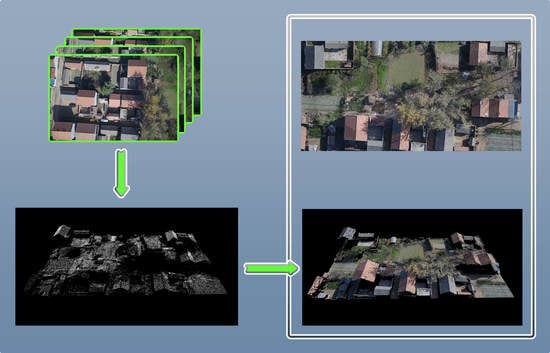
  • This paper presented a top view constrained dense matching method to generate a digital orthophoto without a general 3D reconstruction.
  • The dense matching works on a raster with a top-down propagation significantly improves the generation speed of the digital orthophoto.
  • Testing on various scenes and with some commercial software shows that the method is reliable and efficient.

2. Related Work

Many previous studies analyzed the generation process of the digital orthophoto. In digital photogrammetry, a mature workflow has been widely used for decades: image orientations, feature matching, dense 3D points generation, DEM/DSM production, orthophoto resolution determination (for DEM/DSM interpolation is necessary), and back projection by collinearity condition equations for orthophoto computation [1]. Liu et al. [2] captured the images with an unmanned aerial vehicle (UAV). Their digital orthophoto is generated by the commercial software Pix4D, which is based on the densified 3D point cloud. Without commercial software, Verhoeven et al. [3] used the SfM method to obtain the sparse point cloud and extrinsic parameters and constructed a 3D model with a dense reconstruction algorithm. Then, the 3D model was used to generate an orthophoto from the top view. The digital orthophoto generated by this method is reliable but the dense reconstruction process is redundant for the digital orthophoto. Barazzetti et al. [4] applied epipolar rectification before the 3D reconstruction. To produce a digital orthophoto, they still need the reconstructed 3D model. Wang et al. [5] mainly focused on the edge of buildings in digital orthophotos. They extracted and matched the line segments in the 2D images to rectify the edge of buildings in the 3D model, which is a post-process on the general dense 3D reconstruction. Chen et al. [6] incrementally generate the dense 3D point cloud based on the simultaneous localization and mapping (SLAM) method instead of SfM. The incremental approach has the problems of error accumulation, and their digital orthophoto is still a by-product of the dense 3D reconstruction. Lin et al. [7] also focused on the edge of buildings on the digital orthophotos. They arranged ground control points (GCP) to ensure the accuracy of the edges of the buildings, but their digital orthophotos output is generated after the dense 3D reconstruction. The above methods all used the general dense reconstruction. In the general dense reconstruction, not all information is valuable to the final digital orthophoto, such as the facade of buildings and details smaller than the required spatial resolution scale.
The digital orthophoto generation methods can be simplified in some special applications. Zhao et al. [8] supposed that a scene was a plane. They were inspired by the simultaneous localization and mapping (SLAM) method to fuse images with weighted multiband in real time. The source images were textured on the resulting map by a homography transformation, so the computational cost was low. However, their result could not be seen as a digital orthophoto because the homography matrix was not applicable to objects higher than the ground plane. Lin et al. [9] introduced a new method for digital orthophoto generation and highlighted the plant location. They used the DSM smoothing method to reduce the double mapping and pixelation artifacts. Moreover, they used seamline control to eliminate seam lines that crossed expected plants. They focused on the accuracy in the local area, which met the requirement for agricultural surveys. Other researchers generated digital elevation models (DEMs) instead of 3D models to obtain digital orthophotos. Hood et al. [10] determined image points’ coordinates and transformed them into horizontal coordinates. However, the accuracy was limited by the quality of the DEM. Fu et al. [11] generated a digital elevation model (DEM) by the dense point image matching of aerial images. After interpolating the DEM, the image point coordinates were calculated and translated to scanned coordinates. Then, they generated a digital orthophoto by interpolating the gray values. The interpolation method cannot be widely applied when the DEM is not dense enough. Li et al. [12] proposed a deep learning method to obtain a topological graph of target scenes. The footprints of buildings and the traces of roads were labeled with colors for observation. Such a topological graph is valuable for specific usage, but it is not applicable when more information is required or when the scenes are not buildings and roads. The application of these digital orthophoto generation methods is limited because of their assumptions on the scenes.
Another unavoidable question is the occlusion problem. In each image, there are objects occluded by some other objects, which influenced the choice of color in the result. Amhar et al. [13] generated the digital orthophoto with a digital terrain model (DTM), which can be considered to be the 3D reconstruction result without a texture. They focused on the occlusion problem of the DTM texture process and considered the image visibility to overcome it. Wang et al. [14] also used DTM to generate the digital orthophoto. Their approach to the occlusion problem is to identify which point is valid for a picture pixel when a pixel is assigned multiple points. Zhou et al. [15] generated the digital orthophoto with a digital building model (DBM), which required a 3D reconstruction process to obtain it. For the scene with buildings, the boundary of the occlusion area is usually a line segment, so the boundary of the occlusion area is easier to obtain than in other irregular scenes. They can detect occlusion by the boundary rather than point by point, but their performance improvement is based on the special scene assumption. Oliveira et al. [16] used a triangulated irregular network (TIN) as the input data of their digital orthophoto generation process and the TIN can be considered to be another pattern of the 3D reconstruction result. They used the gradient and visibility of a triangular face to find images suitable for texturing the face. Gharibi et al. [17] rasterized the DSM and set a label for each of the raster cell to indicate its visibility to the source images. They used an adaptive radial sweep method to determine the labels based on the known DSM. These methods considered the occlusion problem at the stage of texturing a 3D model. However, the occlusion detecting methods mentioned above are not applicable to TDM, because TDM is based on a raster instead of the 3D surface model. In this paper, we designed a new occlusion detection method.

3. Methods

The basic idea of TDM is to use sparse 3D points from SFM to generate dense 3D point located on a raster. The top view of the dense 3D points is the result of the digital orthophoto. Each 3D point corresponds to a pixel in the digital orthophoto.

3.1. Sparse 3D Point Generation

SfM is a standard process for generating sparse 3D points [18]. The aim of the SfM process is to look for the feature points in the scene, X i , i = 1 N P , the camera pose of each image, C j , R j , j = 1 N C , and the camera intrinsic matrix K , where
X i = ( X i , Y i , Z i ) T .
C j = ( C x j , C y j , C z j ) T ,
is the pose center of each image I j .
R j = r 11 j r 12 j r 13 j r 21 j r 22 j r 23 j r 31 j r 32 j r 33 j
is the rotation matrix, N P is the number of scene points, and N C is the number of camera poses. The intrinsic matrix of the camera is
K = f 0 u 0 f v 0 0 1 ,
where f is the focal length, and ( u , v ) are the coordinates of principle point.
The SfM algorithm calculates such unknowns by minimizing the following objective function:
f ( p ) = i = 1 N P j = 1 N C λ i j p i j p ^ i j ( R j , C j , X i ) 2 ,
where p = ( R 1 , R 2 , , R N C , C 1 , C 2 , , C N C , X 1 , X 2 , , X N P ) R 6 N C + 3 N P represents N C camera poses and N P 3D points, λ i j represents the constant weights, p i j is the corresponding point of the 3D point X i in image I j , and p ^ i j is obtained by projecting the 3D point X i to image I j . Equation (5) is optimized with the Levenberg–Marquardt algorithm. To ensure that the scale of the sparse point cloud is consistent with the real space, the camera center of each view has a referenced GPS location. The distance between the camera centers and the GPS locations is also a constraint in the nonlinear optimization.
In our study, the images used in the sparse reconstruction were captured by cameras on a UAV. Figure 2 shows a top view of a sparse 3D points generated by the SfM algorithm in a raster with a designed spatial resolution. The 3D sparse points are located in the cells of the raster. Moreover, the elevation value of each cell was stored as a Z-value. If more than one 3D point is mapped to the same cell, only the point with the largest Z i is left for the digital orthophoto generation.

3.2. Rasterization

A complete digital orthophoto is always tiled with several rectangle rasters. Let a raster has H × W cells. The number of rows of the raster is
H = Y m a x Y m i n L p ,
and the number of columns of the raster is
W = X m a x X m i n L p ,
where X m a x and Y m a x are the maximum values of the X- and Y-coordinates in this area, respectively, X m i n and Y m i n are the minimum values of the X- and Y-coordinates of in this area, respectively. The symbol means rounding down. Furthermore, Z m i n and Z m a x are the minimum and the maximum values, respectively, in this area, which are used below. L p is the spatial resolution of the digital orthophoto refers to the cell size.
In the beginning, each 3D point X i in the sparse point cloud is transformed to a corresponding cell P i , whose coordinate is
p x i = X i X m i n L p , p y i = Y i Y m i n L p .
The elevation z i of the cell is initialized as Z i and its matching score M s i is initialized as 1, the maximum possible value of the matching score. These cells with non-zero matching scores are regarded as seeds. For other cells that are not initialized at the first cycle, the value of M s is set to 1 .

3.3. Square Patch Optimization

In the beginning, only seed cells have known elevation values. We use a propagation process to estimate the cells with unknown elevation values by referring to seed cellsȦs demonstrated shown in Figure 3, a seed cell P k and its eight neighbor cells with unknown elevation are packed as a 3 × 3 square patch S R P k with ( p x k l , p y k l ) T and z k l , l = 1 9 . The elevation values of the eight undetermined cells are initialized with the same elevation value of P k .
The coordinate of each cell ( p x k l , p y k l ) T in S R P k is
X k l Y k l Z k l = p x k l L p + X m i n p y k l L p + Y m i n z k l .
If the patch S R P k can be observed in N C k images with the points at
λ j k l u j k l v j k l 1 = K R j [ I | C j ] X k l Y k l Z k l 1 .
( u j k l , v j k l , 1 ) T and ( X k l , Y k l , Z k l , 1 ) T are homogeneous coordinates [19]. Each point ( u j k l , v j k l , 1 ) T is related to a red-green-blue (RGB) pixel value with color ( R j k l , G j k l , B j k l ) . The mean color of the patch in each image is
R j k ¯ G j k ¯ B j k ¯ = k = 1 9 R j k l k = 1 9 G j k l k = 1 9 B j k l / 9 .
Then, we define a vector
V j k = R j k 1 R j k ¯ G j k 1 G j k ¯ B j k 1 B j k ¯ R j k 2 R j k ¯ G j k 2 G j k ¯ B j k 3 B j k ¯ R j k 9 R j k ¯ G j k 9 G j k ¯ B j k 9 B j k ¯
to highlight the color difference of the patch.
We use the vectors to measure the color consistency between the N C k images. One vector is selected as the reference. Then, we compute the cosine distances of the other vectors with the reference. The average distance is the matching score. To select the best reference, we measure
ψ j k = cos 1 Z k C z j C j X k
between the patch and each of the N C k images, where X k = ( X k , Y k , Z k ) T is the coordinate of the seed cell. ψ j k indicates the angle between ( 0 , 0 , 1 ) T and the vector C j X k . We used the image with the minimum ψ j k as the reference.
To measure the similarity of the vectors V j k , j = 1 N C , from N C k images, the matching score is defined as
M s k = j = 1 N C k , j m , j S n k V k m T V j k V k m V j k N C N v k ,
where V k m is the color vector with minimum ψ j k , S n k is the set of indices of the images where the patch S R P k is occluded by some objects, and N v k is the number of elements in S n k . V k m T V j k V k m V j k is the cosine distance between V k m and V j k . The method of occlusion detection is detailed in Section 3.4.
If the M s k of the square patch is higher than a threshold T M s , the cells in the patch S R P k are labeled as seed cells, textured by the color from I m , and the elevation values of the cells are fixed. T M s is set as 0.7 in this stage.
Inspired by Chen’s work [20], if the matching score of the square patch is lower than threshold, all cells in S R P k are packed as a plane π P k , as shown in Figure 4a. The normal vector n k of plane π P k is changed as
n i = cos θ sin ϕ sin θ sin ϕ cos ϕ ,
where θ randomly varies in the range of [ 0 , 360 ) , and ϕ randomly varies in the range [ 0 , 60 ] . Figure 4b shows an example of the randomly changed plane normal. The normal vector is randomly changed at most N T times to find fit elevation values of the cells in S R P k with a matching score higher than the threshold. In our study, N T was set to 7 because if the elevation of the cells to be estimated is close to the seed cell in S R P k , the random change of the normal vector seven times is enough to find a matching score that meets the threshold requirements. If the cells cannot find an expected matching score, the square patch is discarded, and the cells in it will wait for initialization from other seed cells. The seed cells is able to propagate on the continue smooth surface by this strategy. The case that there are no seed cells on a continue surface seldom occurs.
If there are other seed cells in S R P k , as demonstrated in Figure 5, cells without known elevation were initialized as the average elevation of its nearest seed cells. When the cells were packed as a plane to adjust the normal to look for a higher matching score, the elevation of seed cells would not be affected.

3.4. Occlusion Detection

Figure 6a shows a demonstration of the occlusion problem. P 1 and P 2 are two cells of the final digital orthophoto. P 1 is on the ground but P 2 is on the top surface of a building or other objects higher than the ground. For camera C j , they have the same projection position p I . The color of p I comes from the cell P 2 . We cannot use the color p I to estimate cell P 1 , because P 1 is occluded by P 2 .
Because the images were captured by cameras on the UAV, the center of the camera was higher than any objects in the scene. Only the cell with the highest z value was valid if there were more than one cells projected to the same position.
Suppose P k as a seed cell, which is being used for propagation. I j is one of the views of P k , which is being used for computing the matching score. To judge whether I j is occluded, we sampled some points on the connecting line between cell P k and the camera center C j , as shown in Figure 6b. For each sample point X j k n , its orthographic projection is in cell P j k n according to Equation (8). If some Z-coordinates of the sample points are less than the elevation of their corresponding cells, the image I j would be judged as an occluded image for the cell P k . Because the global maximum value of the Z-coordinate is Z m a x , no cells would be higher than Z m a x , and then sample points with Z-coordinates higher than Z m a x would be unnecessary to be checked. On the connecting line P k C j , we define a point X h j k with the Z-coordinate Z m a x . The points for checking occlusion would be sampled only from the line segment P k X h j k . The sample interval is
L S = P k X h j k N o c c + 1 ,
where N o c c is number of sampled points. In our study, N o c c is 5. More samples improve the running time of the method. However, we found that when Nocc equals 5, it is enough to ensure stability.
In the occlusion detection process, to judge whether a cell is occluded, higher cells should be referenced, as shown in Figure 6c, so the digital orthophoto of a scene is generated from high to low. We divide seed cells into 200 levels based on the elevation. The height of each level is
H L = Z m a x Z m i n 200 .
The propagation cycle would be repeated many times in the digital orthophoto generation process. In the first propagation cycle, only seed cells with elevation in the highest elevation level are used for propataion. As the time of propagation increases, seed cells with lower elevation can be used for propagation. In the propagation cycle C p , p = 1 200 , the seed cells with
Z > Z m a x p H L ,
are used for propagation. After the 200 cycles are finished, the propagation is repeated several more times to fill cells without the expected matching score. The threshold of the matching score is decreased by 0.05 in each repeat time in this stage until no more seed cells are found. However, when no more seed cells are found, the digital orthophoto may still have some cells that have not been textured. TDM asserted that the cells which are not textured could not be viewed by any images, and their color is set as black. The generation process of the digital orthophoto from the sparse 3D points is summarized in Algorithm 1.
Algorithm 1: Digital orthophoto generation process.
Remotesensing 15 00177 i001

4. Experiment and Analysis

The images used in the following experiments were taken by a camera on a drone. The position of the camera center of each image is obtained from a differential GPS. The sparse point cloud was generated using the open-source library open Multiple View Geometry (OpenMVG). We test our method on various scenes. In this section, we selected three common scenarios: city, village, and farmland, to demonstrate the digital orthophoto generation. We also verify the effectiveness of occlusion detection with several examples. To evaluate the accuracy of TDM, we compared the results with that of the commercial software ContextCapture, Pix4D, and Altizure 3D. The times used to generate a digital orthophoto at different spatial resolutions were also measured.

4.1. Test on Various Scene

Figure 7 shows some source images that were used to generate the digital orthophoto of a city. The images contain some high buildings.
The digital orthophoto generation process is demonstrated in Figure 8, with the four results sampled in the generation process. Figure 8a is the top view of the sparse 3D points in a raster. Figure 8b is an oblique view of the 3D points. Figure 8c is the top view after the fifth cycle of propagation, in which only seed cells with an elevation higher than Z m a x 5 H L are used for propagation. Figure 8d is the corresponding oblique view of Figure 8c. Figure 8e is the top view after the 200th cycle, where all the seed cells have been used for propagation. There are still some cells whose M s are lower than the threshold T M s . Then the T M s decrease by a specific value in the following propagation cycle to ensure the black holes can be closed. Figure 8g is the top view of the final result. Without considering the elevation of each cell, it is also the result of the digital orthophoto. Figure 8h is an oblique view of the final result. We can find that the parts invisible in the top view are not taken part in the generation.
Figure 9 shows some images used to generate the digital orthophoto of farmland with a factory inside. We use this example to test that the scene has some large areas with less color variation. The generation steps are demonstrated in Figure 10.
We use the images in Figure 11 to test the performance of the elevation estimation, as there are many sloping roofs. The results are shown in Figure 12.
The spatial resolution L p of these three digital orthophotos was 0.04 m, and the generated image sizes of these digital orthophotos were 5398 × 3233 , 3781 × 3565 and 2500 × 1250 pixels, respectively.

4.2. Elevation of the Occlusion Detection

As shown in Figure 8, Figure 10 and Figure 12, the propagation follows a top-down growth strategy. Image pixels used for high-point cloud generation will not participate in the generation of lower-point clouds, thus guaranteeing color consistency constraints when low-point clouds are generated. In this part, we use examples to illustrate the effectiveness of the occlusion detection algorithms. The occluded areas are always adjacent to buildings. Figure 13a,b are two views of the same scene cropped from two aerial images. In Figure 13a, a part of the lawn (pointed by an arrow) is occluded by the nearby building, as shown in Figure 13b.
Figure 13c,d compares the generated digital orthophoto with and without occlusion detection. As shown in Figure 13d, the color of the roof is incorrectly textured on the ground (marked with red ellipses) when the occlusion detection is disabled. Figure 14 and Figure 15 are the other two examples with and without occlusion detection.

4.3. Evaluation of the Accuracy and Efficiency

In this section, we compared the result of TDM with those from the commercial software Pix4D (version 2.0.104), ContextCapture (version 4.4.0.338), and Altizure 3D (version 1.1.79) to evaluate the accuracy of TDM. These are popular software for generating digital orthophotos based on image sequences. In ContextCapture and Altizure 3D, the digital orthophotos are generated after 3D reconstruction. Pix4D can output the digital orthophotos directly from the general dense points reconstruction. We selected part of the village data for comparison. The selected area had a size of 100 m × 50 m, and the spatial resolution was set as 0.04 m.
The digital orthophotos generated by TDM, Pix4D, ContextCapture, and Altizure3D are displayed in Figure 16. The results generated by different methods were similar.
To measure the similarity between the results, we constructed color difference maps between each pair of the results, as shown in Figure 17. The brightness of the pixels in these maps indicates the difference between corresponding pixels in the digital orthophoto results. The color difference map showed that TDM produced the same measurability and visibility of the generated digital orthophoto as those generated by the commercial software. Furthermore, our result is more similar with that of the Pix4D.
Pix4D is considered one of the most outstanding software [21], and our further comparison focuses on Pix4D. For a detailed texture check, we cropped four small areas in the digital orthophoto (Figure 18a). The results are shown in Figure 18b,c. The colors of the ground near the buildings were more acceptable than those of Pix4D. To compare the measurement accuracy, we measured several distances in the digital orthophoto generated by TDM and Pix4D, as shown in Figure 19. The mean square error between the digital orthophoto of TDM and Pix4D is 0.0498 m with the spatial resolution equals 0.04 m. In general, the accuracy of TDM is acceptable according to the comparison with Pix4D.
These two methods were run on a personal computer with an Intel(R) Core(TM) i7-10870H CPU @ 2.20 GHz and an NVIDIA GeForce RTX 2070 with a Max-Q Design. Both Pix4D and TDM are tested without GPU assistance.
Figure 20 shows the time costs of TDM and Pix4D. In Pix4D, we obtained the time cost information from the quality report, and the recorded time was composed of the point cloud densification time, 3D textured mesh generation time, and ortho-mosaic generation time. In TDM the time cost was measured from the end of the sparse reconstruction to the end of the digital orthophoto generation. The time cost of Pix4D was about 1640 s for all spatial resolutions, while TDM became faster as the spatial resolution decreased.
Figure 21 shows parts of the digital orthophoto with a constant 624 × 312 pixels of different spatial resolutions. It appears that the low-resolution digital orthophoto results of Pix4D were downsampled from the high-resolution result. In our results, the low-resolution digital orthophoto generated with less time was still reliable.

5. Conclusions

The digital orthophoto provides location information and accurately displays the texture of the objects on the ground. Therefore, the digital orthophoto is widely used as a base map in a GIS. Currently, the methods of generating digital orthophotos depend on the result of 3D reconstruction, which leads to many redundant calculations. Reducing the redundant measures improves the efficiency of digital orthophoto generation and facilitates the use of maps for situations such as disaster rescue and quick environmental surveys, where rapid response is required.
This paper presented a top view constrained dense matching method named TDM to generate a digital orthophoto without a general 3D reconstruction. We generated the sparse 3D points using the SfM method. Then we built a raster according to the spatial resolution. The raster is initialed by the sparse 3D points and filled by a top-down propagation.Since the process of TDM is on a raster and only one point is saved in each cell, the computation complexity is directly related to the spatial resolution. Moreover, TDM effectively removed the redundant computation in general 3D reconstruction. We tested TDM on various scenes and compared it with commercial software ContextCapture, Pix4D, and Altizure 3D. The results showed that TDM was reliable and efficient. Currently, the TDM is only implemented on the CPU. The efficiency of TDM can be further improved by parallel computing.

Author Contributions

Conceptualization of this study, Methodology, Algorithm implementation, Experiment, Writing—Original draft preparation, Z.Z.; Methodology, Supervision of this study, G.J.; Data curation, Y.L. All authors have read and agreed to the published version of the manuscript.

Funding

This research received no external funding.

Data Availability Statement

Not applicable.

Conflicts of Interest

The authors declare no conflict of interest.

References

  1. Wolf, P.R.; Dewitt, B.A.; Wilkinson, B.E. Elements of Photogrammetry with Applications in GIS; McGraw-Hill Education: New York, NY, USA, 2014. [Google Scholar]
  2. Liu, Y.; Zheng, X.; Ai, G.; Zhang, Y.; Zuo, Y. Generating a high-precision true digital orthophoto map based on UAV images. ISPRS Int. J. Geo-Inf. 2018, 7, 333. [Google Scholar] [CrossRef] [Green Version]
  3. Verhoeven, G.; Doneus, M.; Briese, C.; Vermeulen, F. Mapping by matching: A computer vision-based approach to fast and accurate georeferencing of archaeological aerial photographs. J. Archaeol. Sci. 2012, 39, 2060–2070. [Google Scholar] [CrossRef]
  4. Barazzetti, L.; Brumana, R.; Oreni, D.; Previtali, M.; Roncoroni, F. True-orthophoto generation from UAV images: Implementation of a combined photogrammetric and computer vision approach. ISPRS Ann. Photogramm. Remote. Sens. Spat. Inf. Sci. 2014, 2, 57–63. [Google Scholar] [CrossRef] [Green Version]
  5. Wang, Q.; Yan, L.; Sun, Y.; Cui, X.; Mortimer, H.; Li, Y. True orthophoto generation using line segment matches. Photogramm. Rec. 2018, 33, 113–130. [Google Scholar] [CrossRef]
  6. Chen, L.; Zhao, Y.; Xu, S.; Bu, S.; Han, P.; Wan, G. DenseFusion: Large-Scale Online Dense Pointcloud and DSM Mapping for UAVs. In Proceedings of the 2020 IEEE/RSJ International Conference on Intelligent Robots and Systems (IROS), Las Vegas, NV, USA, 24 October 2020–24 January 2021; pp. 4766–4773. [Google Scholar]
  7. Lin, T.Y.; Lin, H.L.; Hou, C.W. Research on the production of 3D image cadastral map. In Proceedings of the 2018 IEEE International Conference on Applied System Invention (ICASI), Chiba, Japan, 13–17 April 2018; pp. 259–262. [Google Scholar]
  8. Zhao, Y.; Cheng, Y.; Zhang, X.; Xu, S.; Bu, S.; Jiang, H.; Han, P.; Li, K.; Wan, G. Real-Time Orthophoto Mosaicing on Mobile Devices for Sequential Aerial Images with Low Overlap. Remote Sens. 2020, 12, 3739. [Google Scholar] [CrossRef]
  9. Lin, Y.C.; Zhou, T.; Wang, T.; Crawford, M.; Habib, A. New orthophoto generation strategies from UAV and ground remote sensing platforms for high-throughput phenotyping. Remote Sens. 2021, 13, 860. [Google Scholar] [CrossRef]
  10. Hood, J.; Ladner, L.; Champion, R. Image processing techniques for digital orthophotoquad production. Photogramm. Eng. Remote Sens. 1989, 55, 1323–1329. [Google Scholar]
  11. Fu, J. DOM generation from aerial images based on airborne position and orientation system. In Proceedings of the 2010 6th International Conference on Wireless Communications Networking and Mobile Computing (WiCOM), Chengdu, China, 23–25 September 2010; pp. 1–4. [Google Scholar]
  12. Li, Z.; Wegner, J.D.; Lucchi, A. Topological map extraction from overhead images. In Proceedings of the IEEE/CVF International Conference on Computer Vision, Seoul, Republic of Korea, 27 October–2 November 2019; pp. 1715–1724. [Google Scholar]
  13. Amhar, F.; Jansa, J.; Ries, C. The generation of true orthophotos using a 3D building model in conjunction with a conventional DTM. Int. Arch. Photogramm. Remote Sens. 1998, 32, 16–22. [Google Scholar]
  14. Wang, X.; Zhang, X.; Wang, J. The true orthophoto generation method. In Proceedings of the 2012 First International Conference on Agro- Geoinformatics (Agro-Geoinformatics), Shanghai, China, 2–4 August 2012; pp. 1–4. [Google Scholar] [CrossRef]
  15. Zhou, G.; Wang, Y. A new method of occlusion detection to generate true orthophoto. In Proceedings of the 2016 24th International Conference on Geoinformatics, Galway, Ireland, 14–20 August 2016; pp. 1–4. [Google Scholar]
  16. De Oliveira, H.C.; Dal Poz, A.P.; Galo, M.; Habib, A.F. Surface gradient approach for occlusion detection based on triangulated irregular network for true orthophoto generation. IEEE J. Sel. Top. Appl. Earth Obs. Remote Sens. 2018, 11, 443–457. [Google Scholar] [CrossRef] [Green Version]
  17. Gharibi, H.; Habib, A. True Orthophoto Generation from Aerial Frame Images and LiDAR Data: An Update. Remote Sens. 2018, 10, 581. [Google Scholar] [CrossRef] [Green Version]
  18. Moulon, P.; Monasse, P.; Marlet, R. Global fusion of relative motions for robust, accurate and scalable structure from motion. In Proceedings of the IEEE International Conference on Computer Vision, Sydney, NSW, Australia, 1–8 December 2013; pp. 3248–3255. [Google Scholar]
  19. Hartley, R.; Zisserman, A. Multiple View Geometry in Computer Vision; Cambridge University Press: Cambridge, UK, 2003. [Google Scholar]
  20. Shen, S. Accurate multiple view 3d reconstruction using patch-based stereo for large-scale scenes. IEEE Trans. Image Process. 2013, 22, 1901–1914. [Google Scholar] [CrossRef] [PubMed]
  21. Casella, V.; Chiabrando, F.; Franzini, M.; Manzino, A.M. Accuracy assessment of a UAV block by different software packages, processing schemes and validation strategies. ISPRS Int. J. Geo-Inf. 2020, 9, 164. [Google Scholar] [CrossRef]
Figure 1. Digital orthophoto of a part of a village. (a) The digital orthophoto is the top view of some 3D points. (b) Looking at these 3D points from an oblique view.
Remotesensing 15 00177 g001
Figure 2. A top view of sparse 3D points generated by the SfM algorithm in a raster with a designed spatial resolution.
Remotesensing 15 00177 g002
Figure 3. A square patch. The squares represent cells in the raster. The height of the vertical column represents the elevation values of each cell. The column in red represents a seed cell.
Remotesensing 15 00177 g003
Figure 4. (a) Plane composed of the seed cell at the center and eight neighbor cells with unknown elevation. The normal of the plane in (a) is ( 0 , 0 , 1 ) T . (b) Example of a plane whose normal has been randomly changed. The seed cell at the center is fixed, and the elevation of other cells vary with the plane.
Remotesensing 15 00177 g004
Figure 5. A square patch with a seed cell at the center and another seed cell at the corner. For each other cells without known elevation, the elevation is initialized as the average elevation of its neighboring seed cells.
Remotesensing 15 00177 g005
Figure 6. Figures to display the occlusion detection process. (a) A demonstration of the occlusion problem. (b) Figure to explain the sampling method of points on the connecting line between the cell P k and the camera center C j . The distance between neighbor sampled points is the sample interval, L S . To highlight the process of the point sampling, cells other than P k are not drawn in this figure. (c) An example of the occlusion detection process. Because the elevation of P j k 5 is higher than the Z-coordinate of X j k 5 , the image I j is judged as an occluded image. However, if the cell P k is used for propagation before the elevation of P j k 5 is known, the occlusion would not be correctly detected.
Remotesensing 15 00177 g006
Figure 7. Some of the aerial images were used to generate the digital orthophoto of a city.
Remotesensing 15 00177 g007
Figure 8. The beginning, two intermediate, and final results of the generation process. The left column (a,c,e,g) is the top view, and the right (b,d,f,h) is the corresponding oblique view.
Remotesensing 15 00177 g008aRemotesensing 15 00177 g008b
Figure 9. Some of the aerial images were used to generate the digital orthophoto of farmland with a factory inside.
Remotesensing 15 00177 g009
Figure 10. The beginning, two intermediate, and final results of the generation process. The left column (a,c,e,g) is the top view, and the right (b,d,f,h) is the corresponding oblique view.
Remotesensing 15 00177 g010
Figure 11. Some of the aerial images were used to generate the digital orthophoto of a village.
Remotesensing 15 00177 g011
Figure 12. The beginning, two intermediate, and final results of the generation process. The left column (a,c,e,g) is the top view, and the right (b,d,f,h) is the corresponding oblique view.
Remotesensing 15 00177 g012aRemotesensing 15 00177 g012b
Figure 13. An example of the occlusion. A part of the lawn (pointed by an arrow) in (a) is occluded by the nearby building, as shown in (b). (c,d) are digital orthophoto results generated with and without occlusion detection. We use the red ellipse to mark the incorrect texture, as shown in (d).
Remotesensing 15 00177 g013
Figure 14. Digital orthophoto results generated with and without occlusion detection. We use the red ellipses to mark the incorrect texture, as shown in (d). (a) Aerial image. (b) Aerial image. (c) Result with occlusion detection. (d) Result without occlusion detection.
Remotesensing 15 00177 g014
Figure 15. Digital orthophoto results generated with and without occlusion detection. We use the red ellipses to mark the incorrect texture, as shown in (d). (a) Aerial image. (b) Aerial image. (c) Result with occlusion detection. (d) Result without occlusion detection.
Remotesensing 15 00177 g015
Figure 16. Digital orthophotos generated by our algorithm, Pix4D, ContextCapture, and Altizure 3D. (a) Digital orthophoto result generated by TDM. (b) Digital orthophoto result generated by Pix4D. (c) Digital orthophoto result generated by ContextCapture. (d) Digital orthophoto result generated by Altizure 3D.
Remotesensing 15 00177 g016
Figure 17. Color difference map between each of the two results. (a) Color difference map between ContextCapture and TDM. (b) Color difference map between Pix4D and TDM. (c) Color difference map between Altizure 3D and TDM. (d) Color difference map between ContextCapture and Pix4D. (e) Color difference map between ContextCapture and Altizure 3D. (f) Color difference map between Pix4D and Altizure 3D.
Remotesensing 15 00177 g017
Figure 18. Detailed comparison between TDM and Pix4D in the digital orthophotos. (a) Four cropped small areas used for a detailed comparison. The numbers 1–4 correspond to the images from left to right in (b) and (c). (b) Details of Pix4D digital orthophoto. (c) Details of TDM digital orthophoto.
Remotesensing 15 00177 g018aRemotesensing 15 00177 g018b
Figure 19. Comparison of length measurement between TDM and Pix4D. The two images are the digital orthophoto generated by TDM and Pix4D. The number next to each colored line indicates the measured distance. (a) Length measurement of TDM. (b) Length measurement of Pix4D.
Remotesensing 15 00177 g019
Figure 20. Time costs of TDM and Pix4D.
Remotesensing 15 00177 g020
Figure 21. Parts of digital orthophotos with a constant 624 × 312 pixels generated from different spatial resolutions. The left column is the results generated by TDM, and the right is the results generated by Pix4D. (a) L p is 4 cm. (b) L p is 6 cm. (c) L p is 8 cm. (d) L p is 10 cm. (e) L p is 12 cm. (f) L p is 14 cm. (g) L p is 16 cm.
Remotesensing 15 00177 g021aRemotesensing 15 00177 g021b
Disclaimer/Publisher’s Note: The statements, opinions and data contained in all publications are solely those of the individual author(s) and contributor(s) and not of MDPI and/or the editor(s). MDPI and/or the editor(s) disclaim responsibility for any injury to people or property resulting from any ideas, methods, instructions or products referred to in the content.

