Article

Improved Surface Soil Organic Carbon Mapping of SoilGrids250m Using Sentinel-2 Spectral Images in the Qinghai–Tibetan Plateau

1
State Key Laboratory of Soil Erosion and Dryland Framing on the Loess Plateau, Institute of Soil and Water Conservation, Northwest A&F University, Xianyang 712100, China
2
Institute of Soil and Water Conservation, Chinese Academy of Science and Ministry of Water Resources, Xianyang 712100, China
3
Department of Earth and Environmental Science, School of Human Settlements and Civil Engineering, Xi’an Jiaotong University, Xi’an 710049, China
4
Institute of Soil and Water Conservation, Beijing Forestry University, Beijing 100083, China
5
Hydrology and Water Resources Branch Bureau of Shigatsa, Hydrology and Water Resources Geological Bureau of Tibet Autonomous Region, Shigatsa 857000, China
6
Sate Key Laboratory of Hydrology-Water Resources and Hydraulic Engineering, Nanjing Hydraulic Research Institute, Nanjing 210029, China
*
Author to whom correspondence should be addressed.
Remote Sens. 2023, 15(1), 114; https://doi.org/10.3390/rs15010114
Submission received: 16 November 2022 / Revised: 11 December 2022 / Accepted: 22 December 2022 / Published: 25 December 2022
(This article belongs to the Special Issue Remote Sensing in Natural Resource and Water Environment)

Abstract

:
Soil organic carbon (SOC) is a critical indicator for the global carbon cycle and the overall carbon pool balance. Obtaining soil maps of surface SOC is fundamental to evaluating soil quality, regulating climate change, and global carbon cycle modeling. However, efficient approaches for obtaining accurate SOC information remain challenging, especially in remote or inaccessible regions of the Qinghai–Tibet Plateau (QTP), which is influenced by complex terrains, climate change, and human activities. This study employed field measurements, SoilGrids250m (SOC_250m, a spatial resolution of 250 m × 250 m), and Sentinel-2 images with different machine learning methods to map SOC content in the QTP. Four machine learning methods including partial least squares regression (PLSR), support vector machines (SVM), random forest (RF), and artificial neural network (ANN) were used to construct spatial prediction models based on 396 field-collected sampling points and various covariates from remote sensing images. Our results revealed that the RF model outperformed the PLSR, SVM, and ANN models, with a higher determination coefficient (R2 of 0.82 is from the training datasets) and the ratio of performance to deviation (RPD = 2.54). The selected covariates according to the variable importance in projection (VIP) were: SOC_250m, B2, B11, Soil-Adjusted Vegetation Index (SAVI), Normalized Difference Vegetation Index (NDVI), B5, and Soil-Adjusted Total Vegetation Index (SATVI). The predicted SOC map showed an overall decrease in SOC content ranging from 69.30 g·kg−1 in the southeast to 1.47 g·kg−1 in the northwest. Our prediction showed spatial heterogeneity of SOC content, indicating that Sentinel-2 images were acceptable for characterizing the variability of SOC. The findings provide a scientific basis for carbon neutrality in the QTP and a reference for the digital mapping of SOC in the alpine region.

1. Introduction

Soil organic carbon (SOC) is a critical factor for assessing soil quality and provides a key role in the overall carbon pool balance and the global carbon cycle [1]. The carbon stored in soils is three times greater than atmospheric carbon storage, even a slight loss of soil carbon to the atmosphere has a substantial influence on greenhouse gas emissions. SOC has become a focal point for global warming [2,3,4] and carbon neutrality was then proposed for targeting the mitigation of climate change. The soil in high-altitude ecosystems, such as the Qinghai–Tibet Plateau (QTP), is generally characterized by high organic carbon density and great spatial variability [5]. The permafrost on the QTP is undergoing extensive degradation since it is more sensitive to climate warming, which could result in the decomposition of SOC in permafrost by microorganisms, influencing the global greenhouse effect and carbon neutrality [6,7]. Field-measured SOC in the permafrost region of the QTP is limited due to the harsh natural environment and challenging access to the depopulated zone. The content and spatial variability of SOC in the permafrost region (about 40% of the area of the QTP) [8] are unclear due to a lack of reliable in situ data. The movement, turnover and transport of SOC in soil, water and atmosphere have not been deeply investigated due to the unclear spatial distribution of SOC [9]. Thus, a high-resolution SOC map is important for improving the understanding of the SOC movement and sustainably managing QTP ecosystems.
SOC acquisition is typically more accurate with soil sampling and laboratory measurement but these procedures are time- and labor-consuming and are not applicable at a regional scale [10]. Remote sensing data offers an alternative approach for monitoring and mapping SOC content [11]. Related studies indicated that remote sensing data was adequate for retrieving soil and geological properties [12], and provided high potential for regional digital soil mapping. Meng, et al. [13] found hyperspectral sensors can better utilize the spectral properties corresponding to SOC content for organic carbon prediction due to a large number of SOC-sensitive bands and narrower bandwidth. Castaldi, et al. [14] applied the Sentinel-2 data to predict SOC content in cropland regions and depicted SOC variability in farmland using Sentinel-2 images. Lu, et al. [15] predicted SOC distribution in a plantation area using Landsat and related data and provided invaluable methods to accurately predict SOC. As a high-quality multispectral sensor, Sentinel-2 combines extensive coverage (swath width of 290 km) to provide extraordinary terrestrial perspectives, spatial resolution (10–60 m), and minimum five-day global revisit time (twin satellites are in orbit). The data obtained from the Sentinel-2 images demonstrated its capability of monitoring and mapping various soil properties on a global scale [16].
Advancements in digital soil mapping (DSM) have allowed pedologists to interpret soil properties and ecological processes using the machine learning method [17]. These widely used methods include partial least squares regression (PLSR), support vector machines (SVM), random forests (RF), etc., which were used successfully to assess the spatial variability of SOC [18,19]. There are considerable studies using machine learning techniques and remote sensing images for SOC mapping with related soil characteristics and environmental variables [20,21,22]. Ließ, et al. [23] combined a digital elevation model and satellite images to predict SOC stocks with five machine learning methods and found the boosted regression tree approach produced the best overall model. Wang, et al. [24] showed that the RF model increased the predictive ability of high-resolution mapping of SOC stocks.
With an average altitude of nearly 4000 m, the QTP is the world’s largest mountain system and low-latitude permafrost area on earth [25]. The permafrost of the QTP holds a large amount of SOC [26]. However, climate warming has led to permafrost degradation, which changes the content and distribution of SOC [27]. Several studies have attempted to assess the spatial variability of SOC content in the QTP [28,29,30]. High-resolution national soil information grids of China contain a variety of soil factors in different layers and have a spatial resolution of 250 m × 250 m [31] but uncertainties existed in the 250 m data due to its complex topography, poor field accessibility, and sensitive ecological environment [32,33]. As mentioned above, there is no consistency in the applicable model for a specific region, the precision of the model is quite different and the results are not comparable. In the QTP, a field soil survey with the help of remote sensing images is a possible solution for predicting soil spatial variability with high spatial resolution. The aims of this study are to (1) improve the SOC mapping from a coarse spatial resolution of SOC data using an optimal machine learning method with field survey data and Sentinel-2 data; and (2) to obtain spatial variability of the SOC map in the surface of the QTP via digital soil mapping.

2. Materials and Methods

2.1. Study Area

The Qinghai–Tibetan Plateau (Figure 1) covers an area of nearly 2.6 million km2 (26°00′12″–39°46′50″N, 78°18′52″–104°46′59″E). The elevation of the QTP is generally higher than 4000 m above sea level [25] and the QTP is renowned as the “Asian Water Tower”, its freshwater resources play a crucial role in human existence environment and sustainable development of Eastern Asia, Southern Asia, and Central Asia [34,35]. The combination of terrain structure and atmospheric circulation results in a warm and humid climate in the southeast and a cold and dry climate in the northwest of the QTP [36]. Precipitation is mainly concentrated from June to September, reaching more than 70% of the yearly total. Precipitation decreases from 2000 mm in the southeast to <50 mm in the northwest, and temperature has similar pattern with a mean annual temperature of −5.75 to 2.57 °C. The plateau is covered with large areas of alpine steppes and alpine meadows, and shrubs are mainly distributed in the southeast, whereas coniferous and broadleaf forests occur mainly in the south and southeast of the QTP and large bare land exists in the northwest [37].

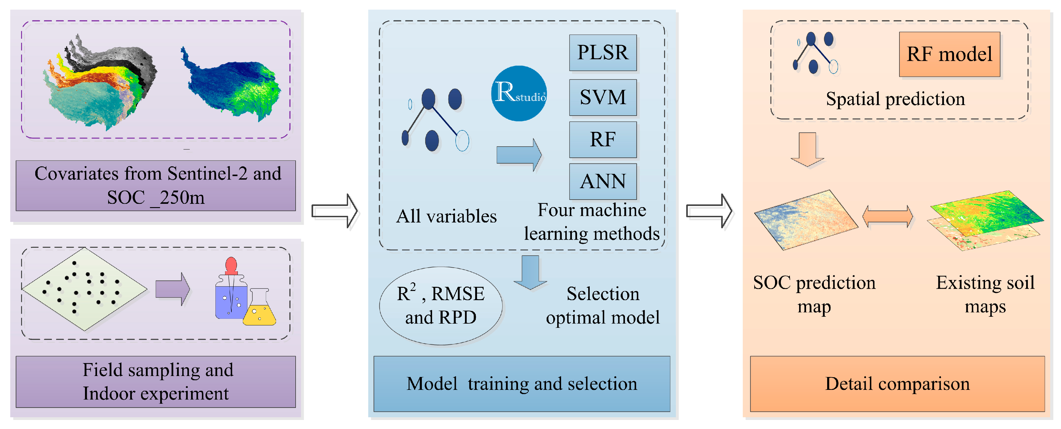
2.2. Methodological Framework

Figure 2 shows the methodological framework involved in our study to model and map SOC concentration in the QTP, including a combination of field measured and machine learning modeling with Sentinel-2 images. In total, we collected 396 surface sampling points to measure the SOC content across the QTP. The field survey attempted to cover as many soil sampling points as possible due to the large stretch of the QTP. Furthermore, we considered different vegetation types, land use, topography and soil types in the whole QTP, and make sure the sampling points represent various soil types. Afterward, a number of potential predicting variables, such as the publicly available SOC data, Sentinel-2 data, vegetation indices, etc. will be selected as input for SOC prediction by machine learning methods. Four different methods including PLSR, SVM, RF, and ANN will be tested to select the optimal approach for SOC spatial prediction. All variables are brought into the optimal RF model and corrected with mtry and ntree to select more important variables. The covariates selected by the VIP were: SOC_250m, B2, B11, SAVI, NDVI, B5, and SATVI for SOC spatial prediction.

2.3. Soil Organic Carbon Data

The SOC data used in this work involve field measured data from the QTP and the Soil Information Grids database from the National Tibetan Plateau Data Center.
Field measured data: a total of 396 surface sampling points were obtained in the QTP from 2019 to 2020 (Figure 1). Three 1 m × 1 m sampling squares were chosen randomly as replicates at each sampling point. Soil samples were obtained at three different locations on the surface sampling square after vegetation aboveground surface crusts and plant litter were removed. Three soil samples from the sampling squares were then mixed into a composite soil sample [38]. Air-dried soils were sieved through a 2 mm screen for analysis in the laboratory. The Walkley–Black dichromate wet-chemistry method was used to estimate the SOC [39].
Soil Information Grid database: The Soil Information Grid database provided a set of specifications for high-resolution national gridded maps across China (https://data.tpdc.ac.cn/zh-hans/ (accessed on 6 December 2021)). Note that many other covariates, such as soil properties, climatic, topographic, etc., were applied to DSM and proved to be useful by Liu, et al. [40]. Our experiments focused on surface SOC prediction by combining the SoilGrids250m (SOC_250m) and the Sentinel-2 images with the optimal machine learning method.

2.4. Environmental Covariates Based on Sentinel-2 Images

Google Earth Engine (GEE) is a cloud-based platform that allows users easy access to powerful computing resources for processing extremely massive geospatial information [41]. It offers an alternating platform for extensive geospatial algorithm advancement, providing higher-impact, data-driven research. We used Sentinel-2 MSI: MultiSpectral Instrument, Level-2A dataset from GEE to obtain spectral reflection data of the QTP. The Sentinel-2 data is a wide-swath, high-resolution, multispectral imaging mission with a global 5-day revisit frequency [42]. The Sentinel-2 data contain 13 spectral bands including visible and near-infrared at 10 m, red edge and SWIR at 20 m, and atmospheric bands at 60 m (Table 1), which can be used to monitor changes in vegetation, soil and water, and inland rivers and coastal locations. Furthermore, the product was pre-processed by European Space Agency (ESA) for radiation calibration, atmospheric correction, etc., ensuring that the data reflects the reflectivity information of the surface, and can be used without subsequent processing after downloading. The Earth Engine Data Catalog (https://developers.google.com/earth-engine/datasets/ (accessed on 24 January 2022)) was used to reference all characteristics of the Sentinel-2 satellite’s multispectral instrument. Based on the timing of our field survey and sampling, we downloaded the atmospherically corrected Sentinel-2 remote sensing images of the QTP with a uniform image spatial resolution of 20 m in the summer season of 2019 and 2020 (from June to September) with the GEE (https://code.earthengine.google.com/ (accessed on 18 May 2022)). As listed in Table 1, a total of 13 bands are available for digital soil mapping, here, we only selected 9 bands (B2, B3, B4, B5, B6, B7, B8A, B11, B12) to predict SOC since the bands B1 and B8 are not suitable for analysis [43]. The B8A was chosen instead of B8 to characterize soil spectral absorption characteristics, which meet the requirements of higher spatial resolution of the study area. Meanwhile, B1 and B9 were not selected since they were used to monitor aerosols in coastal waters and the atmosphere and characterize water vapor [44].
In this study, we calculated environmental factors from Sentinel-2 images using ArcGIS 10.2. Previous studies found that vegetation was an essential determinant influencing SOC content [45,46]. Thus, many vegetation indices were applied for soil digital mapping by combining different bands that can reflect vegetation growth under various conditions. We calculated a variety of relevant vegetation indicators via Sentinel-2 images in this study, including the Normalized Difference Vegetation Index (NDVI), Transformed Vegetation Index (TVI), Enhanced Vegetation Index (EVI), and Soil-Adjusted Vegetation Index (SAVI). The detailed calculation procedures are available in Table 2.

2.5. Models for Soil Organic Carbon Prediction

2.5.1. PLSR

The PLSR is a regression analysis method that allows statistical analysis of multivariate data by allowing simultaneous regression modeling, data structure reduction, and correlation analysis between two sets of variables [20,47]. The main difference between PLSR and ordinary least squares regression is the regression modeling process. PLSR uses data dimensionality reduction, information synthesis, and screening procedures to extract the new integrated components that best explain the system. In linear regression, we assumed that the resulting model y = f (x) is a hyperplane in a space with high dimensions. Assuming that xi ∈ R2 is a two-dimensional vector; then f (x) is a plane. In least squares, we require the error term εi = yif(xi) to have the smallest sum of squares. In fact, |εi| is the distance between the true value yi and the corresponding point f(xi) in the plane.

2.5.2. SVM

The SVM is a classical machine learning model in DSM that has improved the accuracy of predicting soil properties in recent years. It is mainly applied to perform classification and regression analysis on linear, in addition to nonlinear sample data and outlier detection. The data nonlinearity problem can be solved based on the kernel functions to map all sample data into a high-dimensional space with a feature dimension [48]. The SVM can tolerate a maximum divergence ε between f(x) and y, the loss is determined only when the exact value of the gap between f(x) and y is more than ε. This is equivalent to having f(x) at the center, a band of interrogation with a width of 2ε is formed and the training samples are considered to be correctly predicted if they fall into this band.

2.5.3. RF

The RF is composed to perform classification and regression issues using decision trees. The method invoices the idea of ensemble learning (bagging), with the model consisting of a series of regression trees where each tree is trained on a bootstrap sample, and predictions derived by averaging prediction outputs [49]. Specifically, the traditional decision trees select a feature set from each node to obtain the optimal split features, while RF performs the selection of the feature set from the nodes from a randomly generated subset of k features. The parameter k controls the randomness, and here the splitting is the same as the traditional decision tree at k = d. When k = 1, the splitting features are selected randomly. Usually, the recommended value of k is k = log2d [49]. In training, the model must define three parameters: the number of trees in the forest (ntree), the minimum number of data points in each terminal node (node size) and the number of features to try at each node (mtry).

2.5.4. ANN

The ANN is a mathematical model that approximates the organization of synaptic connections in the brain and performs distributed parallel information processing. The model is built on the interconnection of many nodes to construct a neural network that can process massive volumes of data [50]. The ANN regression consists of input layer, hidden layer, and output layer, and linear or non-linear relationships will be established between input or output data. For numerous training sessions, different random beginning points are picked at random, and the outcomes are averaged to obtain the variable importance for each variable.

2.5.5. Model Performance

We took 75% of the 396 surface sampling points as the calibration dataset and 25% as the validation dataset, and preprocessed the calibration and validation dataset separately, including the mean, Kurtosis, CV, etc. The model performances can be quantified by the root mean squared error (RMSE), coefficient of determination (R2), mean absolute error (MAE), and the ratio of performance to deviation (RPD). In the model classification scheme of Chang, et al. [51], when the RPD < 1.0, the model has poor predictive ability and is not recommended; when 1.0 < RPD < 1.4, the model is only sufficient to detect high and low values; when 1.4 < RPD < 2.0, the model is fair, which may be used for evaluation and correlation; when 2.0 < RPD < 2.5, the model displays a very good quantitative; and when RPD > 2.5, the model has excellent prediction ability. All of the modeling and testing for these models were carried out in the RStudio (https://rstudio.com/ (accessed on 27 June 2022)).
R M S E = i = 1 n ( y o y p ) 2 n
M A E = i = 1 n y o y p n
R P D = s t d R M S E
where y o is the observed SOC content (g·kg−1); y p is predicted SOC (g·kg−1); s t d is the standard deviation of the observations; and n is the number of samples.
The model used to predict SOC was chosen by removing redundant covariates and selecting the most relevant covariates, which minimizes model complexity and processing costs [52]. We estimated the significant fraction of the increase in the mean square error (IncMSE) in the RF model. The IncMSE for a particular predictor variable i is determined as a subsequent increase in the mean square error (MSE) of the out-of-bag (OOB) sample due to the fact that predictor i is randomly ranked, while the other predictors remain unchanged [53]. Therefore, the smaller the IncMSE value, the less important the predictor i is.
I n c M S E = M S E i O O B M S E O O B M S E O O B × 100
where M S E O O B is the MSE of OOB samples and M S E i O O B is the MSE of OOB samples when given predictor i is permuted.

3. Results

3.1. Model Performance

As illustrated in Table 3, the measured value of SOC in the total datasets ranged from 0.781 to 84.778 g·kg−1, and the mean value was 17.452 g·kg−1, with a CV of 92.928%. The mean, minimum, maximum, and CV of calibration and validation datasets were similar among the four models (PLSR, SVM, RF, and ANN). The calibration and validation datasets of the four models were randomly selected based on the total datasets and the standard deviation showed some differences between the models. Kurtosis was lower in the validation dataset of the PLSR and RF models, while the calibration dataset of the SVM and ANN models provided a higher kurtosis value.
Figure 3 exhibited stronger linear relationships between the measured and predicted SOC from RF (R2 = 0.82) for model calibration. In general, the RF is optimal among the four models and has strong generality and consistency. In addition to RF, SVM also showed good performance compared to PLSR and ANN, with an R2 higher than 0.6 and an RPD higher than 1.51. PLSR indicated poor stability and generalization among all the models, with the lowest R2 (0.43) and RPD (1.18). The model performance indicated that the RF was the optimal model according to the RMSE, R2, and RPD (Table 4). An RPD > 2.0 implies that the model has a strong prediction ability [51]. Apparently, only RF has the highest prediction ability (RPD = 2.54), suggesting a high potential for SOC prediction when compared to the RPD of the remaining three models. Then, we used the field measurements to analyze with soilGrids250m values, the value of RMSE in the Calibration Dataset was 1.09 higher than RF and the value of R2 was 0.45 lower than the RF model.

3.2. Variable Importance of the Optimal Model

Figure 4 exhibited the ranking of the VIP based on the RF, and a higher IncMSE value indicated more important variables. The SOC_250m was found to be the most relevant predictor based on IncMSE. In addition, the variables with the highest IncMSE value in the nine single bands and the five spectral indices were B2 and SAVI. The variable importance provides some insights into the selection of variables for RF.
The accuracy of the RF model was evaluated by tuning the input variables from 1 to 15. Figure 5 displayed the results of the RF model for tuning parameters. The abrupt changing of mtry was 7, whereas the RMSE was less than 0.84, MAE was less than 0.619, and R2 was higher than 0.62. Accordingly, SOC_250m, B2, B11, SAVI, NDVI, B5, and SATVI were selected for the following estimation. The discrepancies between RMSE, MAE, and R2 fluctuated slightly when the number of trees tuned increased from 300 to 1000 (Figure 5). Furthermore, the lowest RMSE, MAE, and highest R2 value can be detected when ntree = 600.

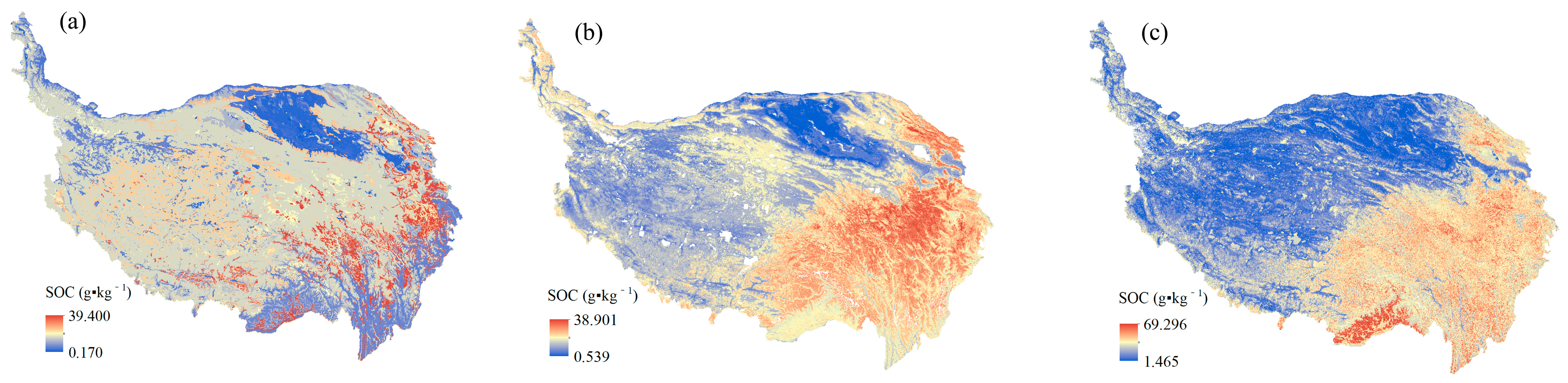
3.3. Spatial Prediction and Mapping of SOC

Figure 6 demonstrates the predicted maps of SOC content at 20 m resolution across the whole QTP. The predicted values of SOC vary from 1.465 to 69.30 g·kg−1, while the field measured SOC varies from 0.781 to 84.78 g·kg−1. Compared with the sampling points in the QTP, the measured values had a wider range than that of the predicted values (Table 3). In general, the SOC content gradually decreases from southeast to northwest in the QTP, the higher values were mostly located in eastern Tibet and the Three Rivers Watershed basin, and the lower values were concentrated in the Qiangtang Plateau and western part of the QTP. The results also indicated that more than 31.34% of the region has a SOC content with a range of 0–10 g·kg−1, and only 2.58% of the region has a SOC content with a range of 50–60 and 60–70 g·kg−1. Overall, the SOC content of the QTP mainly ranged from 1 to 40 g·kg−1.

4. Discussion

4.1. Model Performance and Covariates Selection

This study compared the predictability of PLSR, SVM RF, and ANN models in mapping SOC based on different environmental covariates across the QTP. As shown in Table 4 and Figure 3, the RF model had the highest R2, and the lowest RPD and RMSE. Thus, the performance of the four models developed in our study indicated that the RF model was optimal for the QTP [54]. A similar result was obtained by Heung, et al. [55], who concluded that RF outperformed all other models with a 52% total accuracy average regardless of the sample design. However, it should be noted that the model performance had subtle differences between training and validation, reflecting the problem of over-fitting with limited samples when processing a strong model [24]. Nevertheless, RF performed well in predicting SOC content through multiple decision regression trees. The PLSR has extremely strong applicability in establishing the model of soil fertility index from spectral data [56], while it was not satisfactory in this study. For the linear model, we did not consider the linear relationship between SOC and covariates, especially for the QTP with high variability. Additionally, Were, et al. [57] concluded that the spatial variability of SOC inventory in the Eastern Mau Forest Reserve could be predicted more accurately using SVM rather than RF. Theoretically, land use and topographic attributes are the most significant indicators of SOC content [58,59], the disparity in the two studies is largely dependent on the contrast in vegetation types between forests and alpine meadows. Forkuor, et al. [60] concluded that no single machine-learning method could be optimally suited to different regions. Given that the RF model had relatively high accuracy among all evaluations, the RF model can be applied to predict the variability of SOC in the QTP. Compared to the SOC_250m dataset, our prediction had higher accuracy according to the RMSE and R2.
Until now, multispectral satellite sensors have experienced rapid development in spatial and spectral resolution, especially the new generation of multispectral imaging satellite Sentinel-2 is capable to capture several wavelengths in the SWIR region, including absorption characteristics associated with SOC and soil texture. From the previous studies, the two SWIR (B11 and B12) broad bands are adequate to accurately predict SOM content [14] and SWIR and B5 bands with the highest VIP value [61] have a strong match for SOC prediction in our study (Figure 4). They are related to two organic compounds, lignin and cellulose, affecting the reflectance between 1600 and 1800 nm [62]. Hence, the SWIR performed well in SOC prediction with higher variable importance. Meanwhile, it was also shown that the important distributions of other variables and spectral indices clearly differed from one another. As shown in Figure 4, the B2, SAVIA, and NDVI had higher values in the variable importance, largely influencing the SOC content distribution. This was consistent with Tian, et al. [63], who concluded that the ability of NDVI and EVI to reflect the provision of SOC had an impact on the K factor, which had the same NDVI as our study. Similarly, Ben-Dor, Inbar and Chen [62] indicated that the visible area at 450 nm, 590 nm, and around 664 nm showed a potential relationship between reflectance and organic matter content, which is close to the range of values for the B2 and B5 bands. Only the 30 m resolution shortwave infrared band 5, band 7 and normalized differential water index from 2000–2017 were used in SOC_250m to represent the land surface moisture conditions. In this study, the combination of Sentinel-2 data and the field measurement values of SOC has a strong predictive ability. Thus, the Sentinel-2 data has good potential to predict the spatial pattern of SOC and is applicable in soil digital mapping.

4.2. Spatial Pattern of SOC in the QTP

The variable importance showed that the spatial distribution of SOC was closely linked to a variety of factors (Figure 4), indicating that the correlation between different cofactors and SOC content is fully considered to improve the prediction accuracy by using highly relevant variables for SOC content prediction [64]. Taking into account the spatial and temporal resolution of QTP, it is hard to use the climate and topography as variables input in the model. Meanwhile, the high-resolution National Soil Information Grid of China with a resolution of 250 m explored the link between environment and soil properties, the predictive variables include Landsat (both 5 and 8), MODIS, climate and topography features [40]. Thus, the SOC_250m from Liu et al. [40] was resampled to a raster cell size of 20 m as an input variable combined with our field measured and Sentinel-2 data on the QTP to more accurately predict the distribution of SOC in 2020. Particularly, both the quantile regression forest they used and the RF we used are ensemble tree-based machine learning models that can handle complex nonlinear relationships and multivariate interactions with high predictive power [65]. As shown in Figure 6, the SOC content was higher in the north and lower in the south, gradually increasing from northwest to southeast across the QTP based on these highly relevant variables. Liu, et al. [66] indicated a considerable increase in spatial heterogeneity from northwest to southeast across the QTP, soil organic matter, and remote sensing datasets. Furthermore, the SOC_250m [40] indicated a consistent spatial pattern in the QTP. The difference in the spatial distribution of SOC is largely dependent on land cover type and annual precipitation. Since alpine meadows are primarily found in the eastern portion of the QTP, where biomass and net primary output are substantially higher in the east and lower in the west [67]. Ding, et al. [68] indicated that alpine meadows had a greater mean SOC density than alpine steppes. High precipitation on the eastern QTP also favors the growth of vegetation and the development of permafrost, leading to higher SOC content.
Additionally, the remote sensing images provided by a single sensor can no longer meet the demand for soil characteristics in different geographical and temporal regions and in different dimensions. Multi-source data are required to provide valuable input variables for soil digital mapping [69]. Fortunately, climate change attracted more attention and is certainly associated with SOC [70], advanced multi-source spectral data is now frequently employed for SOC digital mapping. For instance, Gomez, et al. [71] reported that hyperspectral proximal and remote sensing had the potential to predict SOC using visible and near-infrared reflectance. Likewise, a study based on Landsat 8 Monthly NDVI Data found that time series NDVI were helpful to SOC mapping [72]. However, soil roughness, soil moisture, and land cover were important factors influencing the spectral characteristics of images [16]. Similarly, the light source, signal-to-noise ratio, spatial resolution, atmospheric conditions, and pixel cleanliness can also have an impact on remote sensing products [44]. Nevertheless, some studies have overcome many problems and achieved good results to monitor soil properties from Sentinel-2 data [73,74]. The spatial variability of SOC in QTP is consistent with the measured results, which indicated that our results based on Sentinel-2 image data and environmental variables are reliable. Meanwhile, it further indicated that Sentinel-2 has excellent inversion ability of SOC, thus, future research may be expected to predict other soil properties.

4.3. Comparisons with the Existing Soil Map Datasets

Sentinel-2 data provide alternative opportunities to overcome the limitations of traditional soil analysis and sampling with relatively satisfactory results for estimating SOC across the QTP. Furthermore, previous soil maps were used to compare with our results to analyze the accuracy and variability. Figure 7 displayed the spatial distribution of SOC content from the Harmonized World Soil Database (HWSD) [75], Li’s prediction [28], and our prediction. Three SOC content maps in the QTP showed that the contents ranged from 0.170 to 39.400 g·kg−1, 0.539 to 38.901 g·kg−1, and 1.465 to 69.296 g·kg−1, respectively. Although three maps had a consistent trend of spatial patterns, a higher range of SOC content was obviously found in our result. A similar result was examined by Li, et al. [76] who obtained the same result, which showed higher soil organic matter content than that of HWSD in China. Additionally, the 0–30 cm SOC map produced by Shangguan, et al. [77] showed higher SOC content than that of HWSD from land surface modeling. The sampling time should also be responsible for differences between Li’s prediction and our prediction. Their study provided the results of SOC dynamics in various soil layers of China in the early 1980s, 2000s, and early 2010s by using a machine learning method and extensive measuring and our study predicts the content and spatial variability of SOC on the QTP using field sampling and experimental analysis during the period of 2019–2020. In terms of their predicted variation trends, the estimated SOC stocks showed an increasing trend [28].
In order to compare our predictions with others, here, we showed the true color images and different SOC maps in a fixed region with an area of 26 km × 24 km (99.51°–100.85°E and 34.95°–35.93°N) located in the Qinghai Province. As shown in Figure 8, our study produced a 20 m spatial resolution of the SOC map, and HWSD and Li’s prediction had 1 km, which was too coarse to capture the detail of SOC content taxonomic variability. Compared to existing soil map datasets, our prediction has a consistent texture and shape with the image of Sentinel-2, providing more details than other soil maps [78,79]. The SOC map has higher accuracy and could represent SOC variations across the QTP well. Thus, it can be inferred that high-resolution Sentinel-2 images can improve the prediction accuracy in predicting SOC content [80].
It should be noted that our work is limited by the number of validated sampling points. Future research with more sampling data is needed to model training and testing, which will increase the predictability of the model. Moreover, the climatic and topographic properties should be considered in future studies to carry out large-scale SOC monitoring since these variables varied greatly and had a strong influence on soil properties. Meanwhile, future research should also combine multi-source data, including both field measurements, remote sensing images and other variables for soil digital mapping.

5. Conclusions

This study predicted the SOC spatial distribution of the QTP by using four different machine-learning models. The field-measured, Soil Information data (250 m), and Sentinel-2 images were used as model input for training and testing.
The RF model performed best among the four models, with the highest determination coefficient and the ratio of performance to deviation, which can be reasonably applied to the prediction of SOC for the QTP. Our prediction was highly dependent on SOC_250m data, which has the highest importance. B2, B11, SAVI, and NDVI have high VIP among the 14 variables. The SOC map at 20 m resolution suggested an overall decrease ranging from 69.30 g·kg−1 in the southeast to 1.47 g·kg−1 in the northwest in the QTP. Higher values are mostly located in eastern Tibet and the Three Rivers Watershed basin, and lower values are concentrated in the Qiangtang Plateau and the western part of the QTP.
The findings of this study showed high spatial variability of SOC on the QTP at 20 m resolution and are expected to provide a scientific foundation for the distribution and stock of SOC in the QTP region.

Author Contributions

Conceptualization, J.Y. and G.Z.; methodology, J.Y.; software, J.F.; formal analysis, Y.W.; investigation, J.Y. and Z.X.; resources, Y.W.; data curation, J.F., Z.X.; writing—original draft preparation, J.Y. and G.Z.; writing—review and editing, Z.L. and X.M.; visualization, X.M. and P.M.; supervision, G.Z.; project administration, X.M.; funding acquisition, G.Z. All authors have read and agreed to the published version of the manuscript.

Funding

This research was funded by the Strategic Priority Research Program of the Chinese Academy of Sciences (Pan-Third Pole Environment Study for a Green Silk Road) (No: XDA20040202), the National Key Scientific Research Project (Grant No. 2022YFC3201701), and the Western Light Interdisciplinary Team-Key Laboratory Cooperative Research Project, Chinese Academy Sciences “Coupling Processes and Regulation of Water Erosion and Carbon Turnover in the Tibetan Plateau” (Granted in 2020).

Acknowledgments

Thanks are also given to the reviewers for their valuable comments, which significantly improved the paper’s quality.

Conflicts of Interest

There are no conflict of interest in this work.

References

  1. Wang, S.; Guan, K.; Zhang, C.; Lee, D.; Margenot, A.J.; Ge, Y.; Peng, J.; Zhou, W.; Zhou, Q.; Huang, Y. Using soil library hyperspectral reflectance and machine learning to predict soil organic carbon: Assessing potential of airborne and spaceborne optical soil sensing. Remote Sens. Environ. 2022, 271, 112914. [Google Scholar] [CrossRef]
  2. de Anta, R.C.; Luís, E.; Febrero-Bande, M.; Galiñanes, J.; Macías, F.; Ortíz, R.; Casás, F. Soil organic carbon in peninsular Spain: Influence of environmental factors and spatial distribution. Geoderma 2020, 370, 114365. [Google Scholar] [CrossRef]
  3. Melillo, J.M.; Steudler, P.A.; Aber, J.D.; Newkirk, K.; Lux, H.; Bowles, F.P.; Catricala, C.; Magill, A.; Ahrens, T.; Morrisseau, S. Soil Warming and Carbon-Cycle Feedbacks to the Climate System. Science 2002, 298, 2173–2176. [Google Scholar] [CrossRef] [PubMed]
  4. Wang, S.; Zhao, Y.; Wang, J.; Gao, J.; Zhu, P.; Cui, X.a.; Xu, M.; Zhou, B.; Lu, C. Estimation of soil organic carbon losses and counter approaches from organic materials in black soils of northeastern China. J. Soils Sediments 2020, 20, 1241–1252. [Google Scholar] [CrossRef]
  5. Yao, T.; Thompson, L.; Yang, W.; Yu, W.; Gao, Y.; Guo, X.; Yang, X.; Duan, K.; Zhao, H.; Xu, B.; et al. Different glacier status with atmospheric circulations in Tibetan Plateau and surroundings. Nat. Clim. Chang. 2012, 2, 663–667. [Google Scholar] [CrossRef]
  6. Hjort, J.; Streletskiy, D.; Doré, G.; Wu, Q.; Bjella, K.; Luoto, M. Impacts of permafrost degradation on infrastructure. Nat. Rev. Earth Environ. 2022, 3, 24–38. [Google Scholar] [CrossRef]
  7. Wang, Y.; Xu, Y.; Wei, D.; Shi, L.; Jia, Z.; Yang, Y. Different chemical composition and storage mechanism of soil organic matter between active and permafrost layers on the Qinghai–Tibetan Plateau. J. Soils Sediments 2020, 20, 653–664. [Google Scholar] [CrossRef]
  8. Xing, Z.; Fan, L.; Zhao, L.; De Lannoy, G.; Frappart, F.; Peng, J.; Li, X.; Zeng, J.; Al-Yaari, A.; Yang, K.; et al. A first assessment of satellite and reanalysis estimates of surface and root-zone soil moisture over the permafrost region of Qinghai-Tibet Plateau. Remote Sens. Environ. 2021, 265, 112666. [Google Scholar] [CrossRef]
  9. Li, Y.; Liu, W.; Feng, Q.; Zhu, M.; Yang, L.; Zhang, J. Effects of land use and land cover change on soil organic carbon storage in the Hexi regions, Northwest China. J. Environ. Manag. 2022, 312, 114911. [Google Scholar] [CrossRef]
  10. Loiseau, T.; Chen, S.; Mulder, V.L.; Dobarco, M.R.; Richer-de-Forges, A.C.; Lehmann, S.; Bourennane, H.; Saby, N.P.A.; Martin, M.P.; Vaudour, E.; et al. Satellite data integration for soil clay content modelling at a national scale. Int. J. Appl. Earth Obs. Geoinf. 2019, 82, 101905. [Google Scholar] [CrossRef]
  11. Shankar, D.R. Remote Sensing of Soils; Springer: Berlin/Heidelberg, Germany, 2017. [Google Scholar]
  12. Castaldi, F.; Chabrillat, S.; Chartin, C.; Genot, V.; Jones, A.R.; van Wesemael, B. Estimation of soil organic carbon in arable soil in Belgium and Luxembourg with the LUCAS topsoil database. Eur. J. Soil Sci. 2018, 69, 592–603. [Google Scholar] [CrossRef]
  13. Meng, X.; Bao, Y.; Wang, Y.; Zhang, X.; Liu, H. An advanced soil organic carbon content prediction model via fused temporal-spatial-spectral (TSS) information based on machine learning and deep learning algorithms. Remote Sens. Environ. 2022, 280, 113166. [Google Scholar] [CrossRef]
  14. Castaldi, F.; Hueni, A.; Chabrillat, S.; Ward, K.; Buttafuoco, G.; Bomans, B.; Vreys, K.; Brell, M.; van Wesemael, B. Evaluating the capability of the Sentinel 2 data for soil organic carbon prediction in croplands. ISPRS J. Photogramm. Remote Sens. 2019, 147, 267–282. [Google Scholar] [CrossRef]
  15. Lu, W.; Lu, D.; Wang, G.; Wu, J.; Huang, J.; Li, G. Examining soil organic carbon distribution and dynamic change in a hickory plantation region with Landsat and ancillary data. Catena 2018, 165, 576–589. [Google Scholar] [CrossRef]
  16. Dvorakova, K.; Heiden, U.; van Wesemael, B. Sentinel-2 Exposed Soil Composite for Soil Organic Carbon Prediction. Remote Sens. 2021, 13, 1791. [Google Scholar] [CrossRef]
  17. Sadeghi, M.; Babaeian, E.; Tuller, M.; Jones, S.B. The optical trapezoid model: A novel approach to remote sensing of soil moisture applied to Sentinel-2 and Landsat-8 observations. Remote Sens. Environ. 2017, 198, 52–68. [Google Scholar] [CrossRef] [Green Version]
  18. Gomes, L.C.; Faria, R.M.; de Souza, E.; Veloso, G.V.; Schaefer, C.E.G.R.; Filho, E.I.F. Modelling and mapping soil organic carbon stocks in Brazil. Geoderma 2019, 340, 337–350. [Google Scholar] [CrossRef]
  19. Zhu, M.; Feng, Q.; Qin, Y.; Cao, J.; Zhang, M.; Liu, W.; Deo, R.C.; Zhang, C.; Li, R.; Li, B. The role of topography in shaping the spatial patterns of soil organic carbon. Catena 2019, 176, 296–305. [Google Scholar] [CrossRef]
  20. Maynard, J.J.; Levi, M.R. Hyper-temporal remote sensing for digital soil mapping: Characterizing soil-vegetation response to climatic variability. Geoderma 2017, 285, 94–109. [Google Scholar] [CrossRef] [Green Version]
  21. Belgiu, M.; Drăguţ, L. Random forest in remote sensing: A review of applications and future directions. ISPRS J. Photogramm. Remote Sens. 2016, 114, 24–31. [Google Scholar] [CrossRef]
  22. Silveira, C.T.; Oka-Fiori, C.; Santos, L.J.C.; Sirtoli, A.E.; Silva, C.R.; Botelho, M.F. Soil prediction using artificial neural networks and topographic attributes. Geoderma 2013, 195–196, 165–172. [Google Scholar] [CrossRef]
  23. Ließ, M.; Schmidt, J.; Glaser, B. Improving the Spatial Prediction of Soil Organic Carbon Stocks in a Complex Tropical Mountain Landscape by Methodological Specifications in Machine Learning Approaches. PLoS ONE 2016, 11, e0153673. [Google Scholar] [CrossRef] [PubMed] [Green Version]
  24. Wang, B.; Waters, C.; Orgill, S.; Gray, J.; Cowie, A.; Clark, A.; Liu, D.L. High resolution mapping of soil organic carbon stocks using remote sensing variables in the semi-arid rangelands of eastern Australia. Sci. Total Environ. 2018, 630, 367–378. [Google Scholar] [CrossRef] [PubMed]
  25. Baumann, F.; He, J.; Schmidt, K.; Kühn, P.; Scholten, T. Pedogenesis, permafrost, and soil moisture as controlling factors for soil nitrogen and carbon contents across the Tibetan Plateau. Glob. Chang. Biol. 2009, 15, 3001–3017. [Google Scholar] [CrossRef]
  26. Zhao, L.; Wu, X.; Wang, Z.; Sheng, Y.; Fang, H.; Zhao, Y.; Hu, G.; Li, W.; Pang, Q.; Shi, J.; et al. Soil organic carbon and total nitrogen pools in permafrost zones of the Qinghai-Tibetan Plateau. Sci. Rep. 2018, 8, 3656. [Google Scholar] [CrossRef] [Green Version]
  27. Liu, G.; Wu, T.; Hu, G.; Wu, X.; Li, W. Permafrost existence is closely associated with soil organic matter preservation: Evidence from relationships among environmental factors and soil carbon in a permafrost boundary area. Catena 2021, 196, 104894. [Google Scholar] [CrossRef]
  28. Li, H.; Wu, Y.; Liu, S.; Xiao, J.; Zhao, W.; Chen, J.; Alexandrov, G.; Cao, Y. Decipher soil organic carbon dynamics and driving forces across China using machine learning. Glob. Chang. Biol. 2022, 28, 3394–3410. [Google Scholar] [CrossRef]
  29. Ottoy, S.; De Vos, B.; Sindayihebura, A.; Hermy, M.; Van Orshoven, J. Assessing soil organic carbon stocks under current and potential forest cover using digital soil mapping and spatial generalisation. Ecol. Indic. 2017, 77, 139–150. [Google Scholar] [CrossRef]
  30. Zizala, D.; Minařík, R.; Zádorová, T. Soil Organic Carbon Mapping Using Multispectral Remote Sensing Data: Prediction Ability of Data with Different Spatial and Spectral Resolutions. Remote Sens. 2019, 11, 2947. [Google Scholar] [CrossRef]
  31. Liu, F.; Zhang, G.-L.; Song, X.; Li, D.; Zhao, Y.; Yang, J.; Wu, H.; Yang, F. High-resolution and three-dimensional mapping of soil texture of China. Geoderma 2020, 361, 114061. [Google Scholar] [CrossRef]
  32. Ding, J.; Wang, T.; Piao, S.; Smith, P.; Zhang, G.; Yan, Z.; Ren, S.; Liu, D.; Wang, S.; Chen, S.; et al. The paleoclimatic footprint in the soil carbon stock of the Tibetan permafrost region. Nat. Commun. 2019, 10, 4195. [Google Scholar] [CrossRef] [PubMed] [Green Version]
  33. Wang, Z.; Luo, P.; Zha, X.; Xu, C.; Kang, S.; Zhou, M.; Nover, D.; Wang, Y. Overview assessment of risk evaluation and treatment technologies for heavy metal pollution of water and soil. J. Clean. Prod. 2022, 379, 134043. [Google Scholar] [CrossRef]
  34. Qin, J.; Duan, W.; Chen, Y.; Dukhovny, V.A.; Sorokin, D.; Li, Y.; Wang, X. Comprehensive evaluation and sustainable development of water–energy–food–ecology systems in Central Asia. Renew. Sustain. Energy Rev. 2022, 157, 112061. [Google Scholar] [CrossRef]
  35. Immerzeel, W.W.; van Beek, L.P.H.; Bierkens, M.F.P. Climate Change Will Affect the Asian Water Towers. Science 2010, 328, 1382–1385. [Google Scholar] [CrossRef] [PubMed]
  36. Li, G.; Zhang, Z.; Shi, L.; Zhou, Y.; Yang, M.; Cao, J.; Wu, S.; Lei, G. Effects of Different Grazing Intensities on Soil C, N, and P in an Alpine Meadow on the Qinghai—Tibetan Plateau, China. Int. J. Environ. Res. Public Health 2018, 15, 2584. [Google Scholar] [CrossRef] [PubMed] [Green Version]
  37. Gao, Q.; Guo, Y.; Xu, H.; Ganjurjav, H.; Li, Y.; Wan, Y.; Qin, X.; Ma, X.; Liu, S. Climate change and its impacts on vegetation distribution and net primary productivity of the alpine ecosystem in the Qinghai-Tibetan Plateau. Sci. Total Environ. 2016, 554–555, 34–41. [Google Scholar] [CrossRef]
  38. Liu, L.; Zhao, G.; An, Z.; Mu, X.; Jiao, J.; An, S.; Tian, P. Effect of grazing intensity on alpine meadow soil quality in the eastern Qinghai-Tibet Plateau, China. Ecol. Indic. 2022, 141, 109111. [Google Scholar] [CrossRef]
  39. Nelson, D.W.; Sommers, L.E. Total Carbon, Organic Carbon, and Organic Matter. In Methods of Soil Analysis; SSSA Book Series; Soil Science Society of America, Inc.: Madison, WI, USA; American Society of Agronomy, Inc.: Madison, WI, USA, 1996; pp. 961–1010. [Google Scholar] [CrossRef]
  40. Liu, F.; Wu, H.; Zhao, Y.; Li, D.; Yang, J.-L.; Song, X.; Shi, Z.; Zhu, A.X.; Zhang, G.-L. Mapping high resolution National Soil Information Grids of China. Sci. Bull. 2022, 67, 328–340. [Google Scholar] [CrossRef]
  41. Gorelick, N.; Hancher, M.; Dixon, M.; Ilyushchenko, S.; Thau, D.; Moore, R. Google Earth Engine: Planetary-scale geospatial analysis for everyone. Remote Sens. Environ. 2017, 202, 18–27. [Google Scholar] [CrossRef]
  42. Khare, S.; Latifi, H.; Khare, S. Vegetation Growth Analysis of UNESCO World Heritage Hyrcanian Forests Using Multi-Sensor Optical Remote Sensing Data. Remote Sens. 2021, 13, 3965. [Google Scholar] [CrossRef]
  43. Bonansea, M.; Ledesma, M.; Bazán, R.; Ferral, A.; German, A.; O’Mill, P.; Rodriguez, C.; Pinotti, L. Evaluating the feasibility of using Sentinel-2 imagery for water clarity assessment in a reservoir. J. S. Am. Earth Sci. 2019, 95, 102265. [Google Scholar] [CrossRef]
  44. Wang, K.; Qi, Y.; Guo, W.; Zhang, J.; Chang, Q. Retrieval and Mapping of Soil Organic Carbon Using Sentinel-2A Spectral Images from Bare Cropland in Autumn. Remote Sens. 2021, 13, 1072. [Google Scholar] [CrossRef]
  45. Gholizadeh, A.; Žižala, D.; Saberioon, M.; Borůvka, L. Soil organic carbon and texture retrieving and mapping using proximal, airborne and Sentinel-2 spectral imaging. Remote Sens. Environ. 2018, 218, 89–103. [Google Scholar] [CrossRef]
  46. Huete, A.; Didan, K.; Miura, T.; Rodriguez, E.P.; Gao, X.; Ferreira, L.G. Overview of the radiometric and biophysical performance of the MODIS vegetation indices. Remote Sens. Environ. 2002, 83, 195–213. [Google Scholar] [CrossRef]
  47. Taghizadeh-Mehrjardi, R.; Schmidt, K.; Toomanian, N.; Heung, B.; Behrens, T.; Mosavi, A.S.; Band, S.; Amirian-Chakan, A.; Fathabadi, A.; Scholten, T. Improving the spatial prediction of soil salinity in arid regions using wavelet transformation and support vector regression models. Geoderma 2021, 383, 114793. [Google Scholar] [CrossRef]
  48. Cortes, C.; Vapnik, V. Support-vector networks. Mach. Learn. 1995, 20, 273–297. [Google Scholar] [CrossRef]
  49. Breiman, L. Random Forests. Mach. Learn. 2001, 45, 5–32. [Google Scholar] [CrossRef] [Green Version]
  50. Aitkenhead, M.J.; Coull, M.; Towers, W.; Hudson, G.; Black, H.I.J. Prediction of soil characteristics and colour using data from the National Soils Inventory of Scotland. Geoderma 2013, 200–201, 99–107. [Google Scholar] [CrossRef]
  51. Chang, C.-W.; Laird, D.A.; Mausbach, M.J.; Hurburgh, C.R. Near-Infrared Reflectance Spectroscopy–Principal Components Regression Analyses of Soil Properties. Soil Sci. Soc. Am. J. 2001, 65, 480–490. [Google Scholar] [CrossRef]
  52. Sothe, C.; Gonsamo, A.; Arabian, J.; Snider, J. Large scale mapping of soil organic carbon concentration with 3D machine learning and satellite observations. Geoderma 2022, 405, 115402. [Google Scholar] [CrossRef]
  53. Svetnik, V.; Liaw, A.; Tong, C.; Culberson, J.; Sheridan, R.; Feuston, B. Random Forest: A Classification and Regression Tool for Compound Classification and QSAR Modeling. J. Chem. Inf. Comput. Sci. 2003, 43, 1947–1958. [Google Scholar] [CrossRef] [PubMed]
  54. Yang, R.-M.; Zhang, G.-L.; Liu, F.; Lu, Y.-Y.; Yang, F.; Yang, F.; Yang, M.; Zhao, Y.-G.; Li, D.-C. Comparison of boosted regression tree and random forest models for mapping topsoil organic carbon concentration in an alpine ecosystem. Ecol. Indic. 2016, 60, 870–878. [Google Scholar] [CrossRef]
  55. Heung, B.; Ho, H.C.; Zhang, J.; Knudby, A.; Bulmer, C.E.; Schmidt, M.G. An overview and comparison of machine-learning techniques for classification purposes in digital soil mapping. Geoderma 2016, 265, 62–77. [Google Scholar] [CrossRef]
  56. dos Santos, F.R.; de Oliveira, J.F.; Bona, E.; dos Santos, J.V.F.; Barboza, G.M.C.; Melquiades, F.L. EDXRF spectral data combined with PLSR to determine some soil fertility indicators. Microchem. J. 2020, 152, 104275. [Google Scholar] [CrossRef]
  57. Were, K.; Bui, D.T.; Dick, Ø.B.; Singh, B.R. A comparative assessment of support vector regression, artificial neural networks, and random forests for predicting and mapping soil organic carbon stocks across an Afromontane landscape. Ecol. Indic. 2015, 52, 394–403. [Google Scholar] [CrossRef]
  58. Grimm, R.; Behrens, T.; Märker, M.; Elsenbeer, H. Soil organic carbon concentrations and stocks on Barro Colorado Island—Digital soil mapping using Random Forests analysis. Geoderma 2008, 146, 102–113. [Google Scholar] [CrossRef]
  59. Stumpf, F.; Keller, A.; Schmidt, K.; Mayr, A.; Gubler, A.; Schaepman, M. Spatio-temporal land use dynamics and soil organic carbon in Swiss agroecosystems. Agric. Ecosyst. Environ. 2018, 258, 129–142. [Google Scholar] [CrossRef]
  60. Forkuor, G.; Hounkpatin, O.K.L.; Welp, G.; Thiel, M. High Resolution Mapping of Soil Properties Using Remote Sensing Variables in South-Western Burkina Faso: A Comparison of Machine Learning and Multiple Linear Regression Models. PLoS ONE 2017, 12, e0170478. [Google Scholar] [CrossRef] [Green Version]
  61. Gerighausen, H.; Menz, G.; Kaufmann, H. Spatially Explicit Estimation of Clay and Organic Carbon Content in Agricultural Soils Using Multi-Annual Imaging Spectroscopy Data. Appl. Environ. Soil Sci. 2012, 2012, 868090. [Google Scholar] [CrossRef]
  62. Ben-Dor, E.; Inbar, Y.; Chen, Y. The reflectance spectra of organic matter in the visible near-infrared and short wave infrared region (400–2500 nm) during a controlled decomposition process. Remote Sens. Environ. 1997, 61, 1–15. [Google Scholar] [CrossRef]
  63. Tian, Z.; Liu, F.; Liang, Y.; Zhu, X. Mapping soil erodibility in southeast China at 250 m resolution: Using environmental variables and random forest regression with limited samples. Int. Soil Water Conserv. 2022, 10, 62–74. [Google Scholar] [CrossRef]
  64. Meersmans, J.; De Ridder, F.; Canters, F.; De Baets, S.; Van Molle, M. A multiple regression approach to assess the spatial distribution of Soil Organic Carbon (SOC) at the regional scale (Flanders, Belgium). Geoderma 2008, 143, 1–13. [Google Scholar] [CrossRef]
  65. Gyamerah, S.A.; Ngare, P.; Ikpe, D. Probabilistic forecasting of crop yields via quantile random forest and Epanechnikov Kernel function. Agric. For. Meteorol. 2020, 280, 107808. [Google Scholar] [CrossRef]
  66. Liu, S.; Sun, Y.; Dong, Y.; Zhao, H.; Dong, S.; Zhao, S.; Beazley, R. The spatio-temporal patterns of the topsoil organic carbon density and its influencing factors based on different estimation models in the grassland of Qinghai-Tibet Plateau. PLoS ONE 2019, 14, e0225952. [Google Scholar] [CrossRef] [Green Version]
  67. Luo, T.; Li, W.; Zhu, H. Estimated biomass and productivity of natural vegetation on the Tibetan plateau. Ecol. Appl. 2002, 12, 980–997. [Google Scholar] [CrossRef]
  68. Ding, J.; Chen, L.; Ji, C.; Hugelius, G.; Li, Y.; Liu, L.; Qin, S.; Zhang, B.; Yang, G.; Li, F.; et al. Decadal soil carbon accumulation across Tibetan permafrost regions. Nat. Geosci. 2017, 10, 420–424. [Google Scholar] [CrossRef] [Green Version]
  69. Mouazen, A.M.; Shi, Z. Estimation and Mapping of Soil Properties Based on Multi-Source Data Fusion. Remote Sens. 2021, 13, 978. [Google Scholar] [CrossRef]
  70. Polyakov, V.; Lal, R. Modeling soil organic matter dynamics as affected by soil water erosion. Environ. Int. 2004, 30, 547–556. [Google Scholar] [CrossRef]
  71. Gomez, C.; Rossel, R.A.V.; McBratney, A.B. Soil organic carbon prediction by hyperspectral remote sensing and field vis-NIR spectroscopy: An Australian case study. Geoderma 2008, 146, 403–411. [Google Scholar] [CrossRef]
  72. Zhang, Y.; Guo, L.; Chen, Y.; Shi, T.; Luo, M.; Ju, Q.; Zhang, H.; Wang, S. Prediction of Soil Organic Carbon based on Landsat 8 Monthly NDVI Data for the Jianghan Plain in Hubei Province, China. Remote Sens. 2019, 11, 1683. [Google Scholar] [CrossRef] [Green Version]
  73. Liu, Y.; Jiaxin, Q.; Yue, H. Comprehensive Evaluation of Sentinel-2 Red Edge and Shortwave-Infrared Bands to Estimate Soil Moisture. IEEE J. Sel. Top. Appl. Earth Obs. Remote Sens. 2021, 14, 7448–7465. [Google Scholar] [CrossRef]
  74. Vaudour, E.; Gilliot, J.M.; Bel, L.; Lefevre, J.; Chehdi, K. Regional prediction of soil organic carbon content over temperate croplands using visible near-infrared airborne hyperspectral imagery and synchronous field spectra. Int. J. Appl. Earth Obs. Geoinf. 2016, 49, 24–38. [Google Scholar] [CrossRef]
  75. Fischer, G.F.; Nachtergaele, S.; Prieler, H.T.; van Velthuizen, L.; Verelst, D.; Wiberg. Global Agro-Ecological Zones Assessment for Agriculture (GAEZ 2008); IIASA: Laxenburg, Austria; FAO: Rome, Italy, 2018. [Google Scholar]
  76. Li, Q.; Yue, T.; Wang, C.; Zhang, W.; Yu, Y.; Li, B.; Yang, J.; Bai, G. Spatially distributed modeling of soil organic matter across China: An application of artificial neural network approach. Catena 2013, 104, 210–218. [Google Scholar] [CrossRef]
  77. Shangguan, W.; Dai, Y.; Liu, B.; Zhu, A.; Duan, Q.; Wu, L.; Ji, D.; Ye, A.; Yuan, H.; Zhang, Q.; et al. A China data set of soil properties for land surface modeling. J. Adv. Model. Earth Syst. 2013, 5, 212–224. [Google Scholar] [CrossRef]
  78. Li, F.; Peng, Y.; Chen, L.; Yang, G.; Abbott, B.W.; Zhang, D.; Fang, K.; Wang, G.; Wang, J.; Yu, J.; et al. Warming alters surface soil organic matter composition despite unchanged carbon stocks in a Tibetan permafrost ecosystem. Funct. Ecol. 2020, 34, 911–922. [Google Scholar] [CrossRef]
  79. Sanchez, P.A.; Ahamed, S.; Carré, F.; Hartemink, A.E.; Hempel, J.; Huising, J.; Lagacherie, P.; McBratney, A.B.; McKenzie, N.J.; Mendonça-Santos, M.d.L.; et al. Digital Soil Map of the World. Science 2009, 325, 680–681. [Google Scholar] [CrossRef] [PubMed] [Green Version]
  80. Urbina-Salazar, D.; Vaudour, E.; Baghdadi, N.; Ceschia, E.; Richer-de-Forges, A.C.; Lehmann, S.; Arrouays, D. Using Sentinel-2 Images for Soil Organic Carbon Content Mapping in Croplands of Southwestern France. The Usefulness of Sentinel-1/2 Derived Moisture Maps and Mismatches between Sentinel Images and Sampling Dates. Remote Sens. 2021, 13, 5115. [Google Scholar] [CrossRef]
Figure 1. Distribution of sampling points in the QTP.
Remotesensing 15 00114 g001
Figure 2. Methodological flowchart for SOC prediction.
Remotesensing 15 00114 g002
Figure 3. Predicted and observed SOC for the calibration dataset.
Remotesensing 15 00114 g003
Figure 4. The variable importance projection values distribution in RF.
Remotesensing 15 00114 g004
Figure 5. RF accuracy during the variable selection process using the different numerous trees (ntree).
Remotesensing 15 00114 g005
Figure 6. Spatial variability of SOC in the QTP.
Remotesensing 15 00114 g006
Figure 7. Comparison of SOC mapping results with the existing maps ((a) HWSD, (b) Li’s prediction, (c) Our prediction).
Remotesensing 15 00114 g007
Figure 8. Comparisons of (a) HWSD, (b) Li’s prediction, (c) Our prediction, and (d) true color image.
Remotesensing 15 00114 g008
Table 1. Characteristics of the Sentinel-2 satellite.
Sentinel-2 BandsWavelength
(nm)
Resolution
(m)
Description
B1443.960Aerosol
B2496.610Blue
B3560.010Green
B4664.510Red
B5703.920Red Edge 1
B6740.220Red Edge 2
B7782.520Red Edge 3
B8835.110NIR
B8A864.820Red Edge 4
B9945.020Water vapor
B111613.720SWIR1
B122202.420SWIR2
Table 2. Definition and calculation of the selected spectral indices.
IndexDefinitionCalculation Based on
Sentinel-2 Image Bands
NDVI N I R R e d N I R + R e d B 8 B 4 B 8 + B 4
TVI 0.5 + ρ N I R ρ R e d ρ N I R + ρ R e d × 100 0.5 + B 8 B 4 B 8 + B 4 × 100
EVI ρ N I R ρ R e d ρ N I R + 6 × ρ R e d 7.5 × ρ B l u e + 1 × 2.5 B 8 B 4 B 8 + 6 × B 4 7.5 × B 2 + 1 × 2.5
SATVI ρ S W I R 1 ρ R e d ρ S W I R 1 + ρ R e d + 1 × 2 ρ S W I R 2 2 B 11 B 4 B 11 + B 4 + 1 × 2 B 12 2
SAVI ( ρ N I R ρ R e d ) × 1.5 ρ N I R + ρ R e d + 0.5 ( B 8 B 4 ) × 1.5 B 8 + B 4 + 0.5
Table 3. Description of SOC predictions from four models.
ModelSamplesMean
(g·kg−1)
Min (g·kg−1)Max (g·kg−1)SD (g·kg−1)KurtosisCV (%)
Total17.4520.78184.77816.2183.68192.928
PLSRCalibration17.4880.78184.77816.2893.97293.140
Validation17.3371.10772.72016.0782.93192.733
SVMCalibration17.3890.78181.94015.9523.56291.736
Validation17.6221.10084.77816.9914.08496.418
RFCalibration17.4640.78184.77816.3463.95393.597
Validation17.4141.14571.80515.8952.92991.279
ANNCalibration17.3890.78181.94015.9523.56291.736
Validation17.6221.10084.77816.9914.08496.418
Table 4. Model prediction performance statistics.
ModelCalibration DatasetValidation DatasetRPDRegression
RMSEC (g·kg−1)RC2RMSEV (g·kg−1)RV2
PLSR0.8710.4320.9420.2421.185y = 0.480x + 6.753
SVM0.9030.6191.1480.5061.511y = 0.507x + 6.118
RF0.4560.8230.8700.5762.537y = 0.622x + 4.911
ANN1.0670.4911.0560.5971.270y = 0.437x + 7.919
SOC_250m1.0880.4511.0930.4000567y = 1.176x − 0.702
Disclaimer/Publisher’s Note: The statements, opinions and data contained in all publications are solely those of the individual author(s) and contributor(s) and not of MDPI and/or the editor(s). MDPI and/or the editor(s) disclaim responsibility for any injury to people or property resulting from any ideas, methods, instructions or products referred to in the content.

