A Context Feature Enhancement Network for Building Extraction from High-Resolution Remote Sensing Imagery

Abstract

The complexity and diversity of buildings make it challenging to extract low-level and high-level features with strong feature representation by using deep neural networks in building extraction tasks. Meanwhile, deep neural network-based methods have many network parameters, which take up a lot of memory and time in training and testing. We propose a novel fully convolutional neural network called the Context Feature Enhancement Network (CFENet) to address these issues. CFENet comprises three modules: the spatial fusion module, the focus enhancement module, and the feature decoder module. First, the spatial fusion module aggregates the spatial information of low-level features to obtain buildings’ outline and edge information. Secondly, the focus enhancement module fully aggregates the semantic information of high-level features to filter the information of building-related attribute categories. Finally, the feature decoder module decodes the output of the above two modules to segment the buildings more accurately. In a series of experiments on the WHU Building Dataset and the Massachusetts Building Dataset, our CFENet balances efficiency and accuracy compared to the other four methods we compared, and achieves optimality on all five evaluation metrics: PA, PC, F1, IoU, and FWIoU. This indicates that CFENet can effectively enhance and fuse buildings’ low-level and high-level features, improving building extraction accuracy.

1. Introduction

With the advancement of earth observation technology, the quality and quantity of high-resolution remote sensing data are constantly improving. The generation of high-resolution remote sensing images has made more convenient and detailed data sources available for its applications. Building extraction from high-resolution remote sensing images is a conversion process from data to information. In urban remote sensing, building extraction can be applied to urban and rural planning [1,2]. In surveying and mapping engineering, building extraction is widely used as a means of acquiring data [3,4]. At the same time, it is also an important part of the fields of precision agriculture and environmental monitoring [5,6,7]. However, the buildings in high-resolution remote sensing images have variable shapes, rich details, and inconsistent texture colors. The complexity of imaging conditions and spatial environment poses severe challenges to the automatic extraction of buildings [8,9].

The automated extraction of buildings from high-resolution images has been a challenging topic in the field of remote sensing image processing [10]. The ground object environment in high-resolution remote sensing images is far more complex than the target environment in general images. The proportion of targets to be segmented in remote sensing images is far less than that in general images. For the segmentation task of remote sensing images, the main difficulty lies in the changeable environment of the objects and the small and dense characteristics of the objects to be segmented. At present, building extraction methods can be broadly divided into two categories: the traditional building extraction method and the learning-based building extraction method.

The traditional building extraction methods mainly use hand-designed features such as texture features, geometric features, and spatial information features of buildings in remote sensing images to solve the problem of building extraction. Li et al. [11] utilized integrating saliency cues to extract buildings from remote sensing images in two steps. First, classical features (color, shadow, shape, etc.) were used to identify the initial candidate buildings, and then a significance estimation algorithm was used to filter out the final buildings. Chen et al. [12] first segmented the images to generate candidate buildings by an algorithm combining threshold watershed transformation and hierarchical merging, and then used their proposed edge regularity index and shadow line index to capture the characteristics of buildings, and finally they employed three classifiers to recognize the buildings in the images. Inglada et al. [13] used a machine learning method to perform pixel-level classification of high-resolution remote sensing images with different geometric features to distinguish buildings. Ding et al. [14] presented a building extraction model based on an image segmentation algorithm and geometric feature constraints combined with the Morphological Building Index (MBI). Katartzis et al. [15] used a semantic segmentation algorithm combined with the Markov model and edge corner detection to extract buildings. Awrangjeb et al. [16] proposed a threshold-based automatic evaluation system to segment buildings according to the correspondence between buildings.

The main drawback of the traditional building extraction method is that they heavily rely on the design and implementation of hand-crafted features and require some complex strategies to overcome noise and outlier variations, which increase computational costs and have poor generalization capabilities. Moreover, high-resolution remote sensing images have complex ground object information. It is difficult to accurately describe building information based only on manual-designed features, which results in low building extraction accuracy.

As a widely used deep learning architecture [17,18,19], combining remote sensing technology and deep learning has become a prevalent method in building extraction from high-resolution remote sensing images. The mainstream CNNs are VGGNet [20], ResNet [21], InceptionNet [22], DenseNet [23], AlexNet [24], etc. They have also become the commonly used baseline networks for many newly proposed segmentation models. Jonathan Long et al. [25] proposed the Fully Convolutional Network (FCN) for image pixel-level classification to overcome the limitations of CNN in fine image segmentation. The core difference between FCN and CNN is that FCN replaces the fully connected layer at the end of the CNN-based classification network with the convolution layer. After FCN was proposed, many researchers also proposed some improved image semantic segmentation models based on FCN, such as SegNet [26], DeconvNet [27], U-Net [28], DeepLab [29], PSPNet [30], HRNet [31], etc. Guo et al. [32] added an attention layer to U-Net and used multiple losses to extract complete buildings. Chen et al. [33] proposed a new neural network by combining DeepLabv3+Net with a densely connected convolutional neural network and residual structure. Shao et al. [34] introduced atrous convolution in U-Net to extract buildings and proposed a new residual refinement module to refine the extraction results further. Xu et al. [35] applied the guided filter to a deep neural network to improve the extraction accuracy of diverse objects in urban areas. Zhu et al. [36] proposed a multiple attending path network (MAP-NET) to extract building footprints by learning multi-scale features through multiple parallel paths, followed by applying an attention module and a pyramidal space pool module to obtain global dependencies. Liao et al. [37] combined building contour information and multi-scale semantic information to enhance the robustness of building extraction. Yang et al. [38] presented a novel encoder-decoder structure combining attention mechanism and DenseNets, which fuses features of buildings from different levels through a spatial attention module. Wen et al. [39] proposed an improved method based on the Mask Region Convolutional Neural Network (Mask R-CNN) to detect the boundaries of buildings in complex backgrounds. Zheng et al. [40] added a self-created symmetric information collection module in Deeplabv3+ to reduce noise in images for accurate segmentation of side-scan sonar remote sensing images. Yu et al. [41] proposed a method based on Transformer and YOLOv5 for real-time object detection on side-scan sonar remote sensing images.

Although these FCN-based methods have made considerable progress in the extraction accuracy of buildings, there are still some problems. First, high-resolution remote sensing images contain complex ground object information; different buildings have different shapes, inconsistent colors, and textures, making FCN-based networks fail to extract strong feature representations of buildings. Secondly, FCN-based networks often contain a large number of parameters, which causes the network model to occupy a large memory space during training and testing.

To sum up, the traditional building extraction methods rely excessively on manual-designed features, which are deficient in robustness and accuracy. The learning-based building extraction methods cannot effectively enhance and fuse low-level and high-level features from neural networks and often contain a large number of network structure parameters. In this paper, to better address the above issues, we design a Context Feature Enhancement Network (CFENet) that can learn more contextual information to achieve accurate localization segmentation of buildings. The contributions of this paper can be summarized as follows:

• An end-to-end context feature enhancement network, namely CFENet, is proposed to address the challenges of complexity and diversity of buildings encountered in building extraction from remote sensing images.
• CFENet achieves more accurate building extraction results on the WHU Building Dataset [42] and the Massachusetts Building Dataset [43] by explicitly establishing rich contextual relationships on low-level and high-level features.
• CFENet balances efficiency and accuracy by employing dilated convolution in the spatial fusion module and asymmetric convolution in the focus enhancement module.

The following sections are arranged as follows. Our CFENet is introduced in detail in Section 2. The experiments results of CFENet and the other four methods are analyzed in detail in Section 3, including comparative experiments and ablation experiments. Section 4 discusses the efficiency of different methods and the heatmaps verifying the effectiveness of our proposed modules. Finally, a summary of the entire text is presented in Section 5.

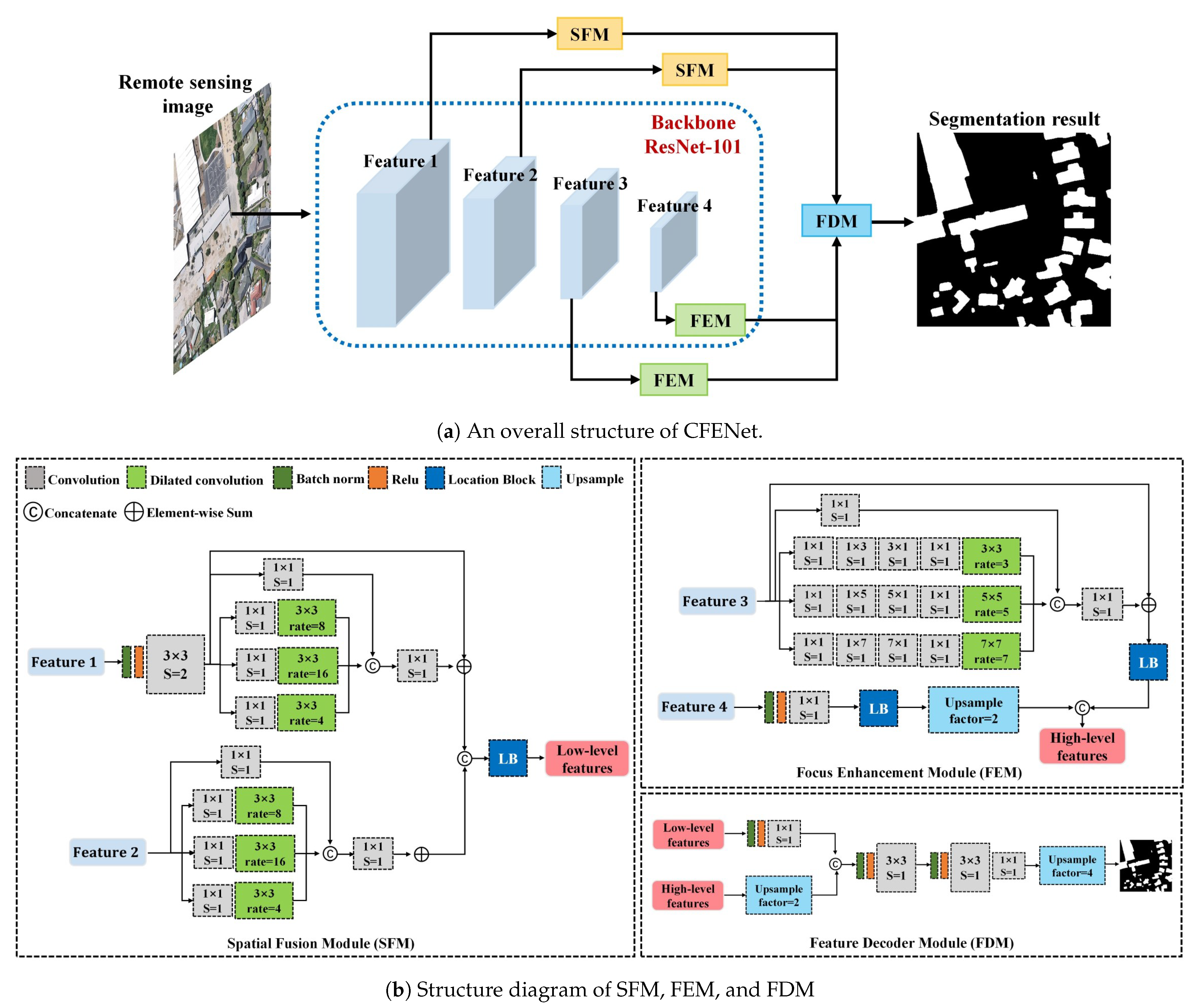
2. The Proposed Context Feature Enhancement Network

2.1. Model Description

Automated extraction of buildings from high-resolution remote sensing images poses serious challenges. The observation mentioned above motivates us to introduce an efficient end-to-end Context Feature Enhancement Network (CFENet), to learn more contextual information to achieve accurate localization segmentation of buildings. The pipeline of CFENet is shown in Figure 1.

CFENet adopts ResNet-101 as the backbone, and the input image size is 512 × 512 pixels. After performing feature extraction through ResNet-101, four different size feature maps are obtained, denoted as Feature 1, Feature 2, Feature 3, and Feature 4. Feature 1 and Feature 2 are low-level features, while Feature 3 and Feature 4 are high-level features. The low-level features contain larger spatial resolution and more detailed information (color, outline, texture, etc.) by employing fewer convolution layers and downsampling operations. However, the low-level features are not rich in semantic information and contain much noisy information. On the contrary, the high-level features have more abstract and rich semantic information (attributes, categories, etc.) by employing more convolution layers and downsampling operations. However, the spatial resolution of the high-level features is small, and spatial information loss is serious.

Our CFENet aggregates the spatial information of low-level features through the spatial fusion module to obtain buildings’ outline and edge information. The focus enhancement module fully integrates the semantic information of the last two high-level features extracted from ResNet-101 to obtain the attribute category information of the building. After the feature encoding of Feature 1 and Feature 2 by the spatial fusion module and the feature encoding of Feature 3 and Feature 4 by the focus enhancement module, CFENet applies the feature decoder module to the outputs of the two modules and performs final decoding to segment accurate buildings.

2.2. Spatial Fusion Module

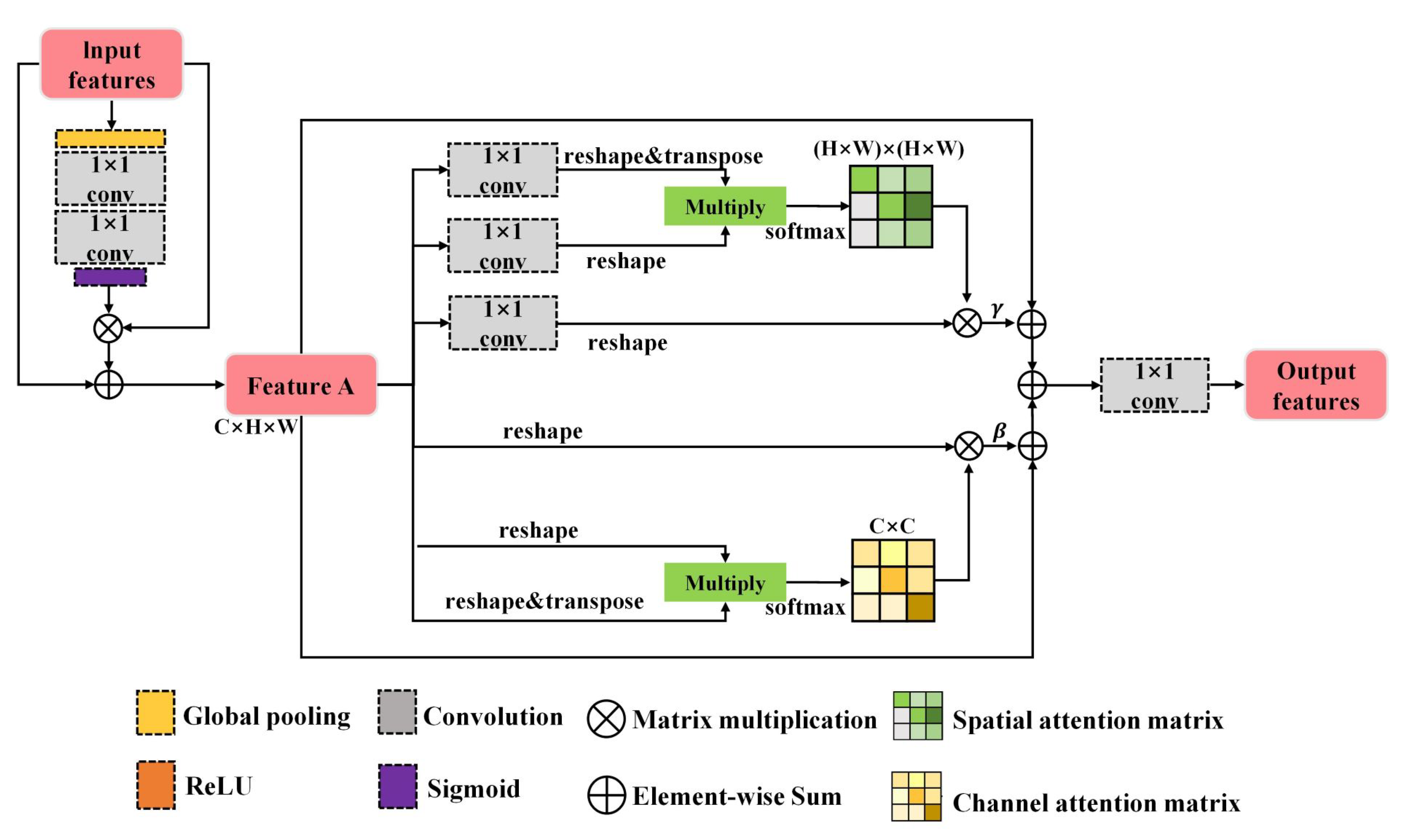
The proposed dilated convolution [44] significantly reduces the drawbacks associated with CNNs. Aiming at the problem of image resolution reduction and information loss caused by downsampling in the task of image semantic segmentation, dilated convolution proposes a new convolution idea. This idea expands the receptive field and reduces the number of network parameters. In this module, we superimpose dilated convolutions with different dilated rates to simulate different receptive fields according to the characteristics of dilated convolution and enhance the representational ability of features by concatenating the features of different receptive fields.

Because the low-level features are applied with fewer convolution layers and downsampling operations, they usually contain greater spatial resolution and richer spatial information (color, outline, texture, etc.). To better extract the spatial information of buildings from low-level features, we increase the receptive field by using dilated convolutions with different dilation rates. The details of the spatial fusion module are illustrated in Figure 1b.

In our work, $\left\{F_i|i=\{1,2,3,4\}\right\}$ are the features of different stages extracted by the backbone network. $F_1$ and $F_2$ are respectively fed into the two branches, and then fed into the Location Block after concatenation to obtain enhanced low-level features $f_{low}$:

$$f_{low}=\Phi \left(C\left\{{\delta }_{\theta }\left(F_1\right),{\phi }_{\theta }\left(F_2\right)\right\}\right)$$

(1)

where ${\delta }_{\theta }$ represents the first branch of the spatial fusion module, ${\phi }_{\theta }$ represents the second branch of the spatial fusion module. C represents concatenation operation, and $\Phi$ represents the Location Block.

The design of the spatial fusion module is based on multi-branch dilated convolution. The input of this module is Feature 1 (number of channels: 256, feature map size: 128 × 128) and Feature 2 (number of channels: 512, feature map size: 64 × 64). First, by using a 3 × 3 convolution layer with a step size of 2 to keep Feature 1 the same size as Feature 2, and then through a parallel branch, which has four branches $\left\{branc{h}_k,k=1,2,3,4\right\}$. A 1 × 1 convolution layer is used in each branch to reduce the number of channels in the feature map. When k > 1, a 3 × 3 dilated convolution layer is added after the 1 × 1 convolution layer in each branch, and the dilation ratio is set to $2^k$. Subsequently, the output features of the four branches are aggregated through a concatenation operation, and then the dimensionality is reduced by a 1 × 1 convolution layer. Finally, the dimensionality reduction features are added element-by-element with the features before entering the branch. Like Feature 1, Feature 2 also needs to go through the same parallel branch. The difference is that Feature 2 does not need to perform any operations before entering the parallel branch. Finally, Feature 1 and Feature 2 are concatenated together, and then the concatenated features are fed into the Location Block for feature enhancement. The Location Block is described in detail in Section 2.3.

2.3. Location Block

In this paper, we propose a unit named Location Block (LB) based on the idea of the Dual Attention Network [45] combined with the channels Squeeze-Extraction [46] operation, which improves the performance of the network by enabling it to execute feature recalibration adaptively. The main function of Location Block is to enhance the essential features and weaken the non-essential features, so as to make the extracted features more powerfully representational. In addition, a parallel module enables the network to learn the mapping relationship between interdependent channels and the correlation degree between each pixel in the feature map. The architecture of the Location Block is shown in Figure 2.

The Location Block first performs a global pooling operation on the input features, followed by the first 1 × 1 convolution layer to squeeze the C channels into C/r channels to reduce the amount of computation, and the second 1 × 1 convolution layer is restored back to C channels, where r refers to the compression ratio, which is set to 16 in this paper. The next step is the reweight operation. The weight output by the sigmoid function is considered to the feature channels’ importance after feature reselection. The weight is then multiplied channel-by-channel to the previous features, thus completing the recalibration of the original features in the channel dimension. We perform the above operations to model the feature channel-wise dependencies as completely as possible.

After completing the above steps, we design two parallel branches to capture rich long-range contextual relationships in spatial and channel dimensions, in order to obtain better intra-class consistent feature representation. We first introduce the first branch. $\mathit{A}\in {\mathbb{R}}^{C\times H\times W}$ is the feature map of the input parallel module. First, feature A is converted into new features B, C, and D by the 1 × 1 convolution layer, where $\left\{\mathit{B},\mathit{C},\mathit{D}\right\}\in {\mathbb{R}}^{C\times H\times W}$. Then both feature maps B and C are reshaped to ${\mathbb{R}}^{C\times N}$, where $N=H\times W$. The transposed B is then multiplied by C and a softmax activation function is applied to obtain a spatial attention map $\mathit{S}\in {\mathbb{R}}^{N\times N}$:

$$s_{ji}=\frac{exp\left(B_i^T·C_j\right)}{{\sum }_{i=1}^{N}exp\left(B_i^T·C_j\right)}$$

(2)

where the impact of the jth pixel on the ith pixel denotes the value of $s_{ji}$. The more similar the feature representations of the two positions are, the greater their correlation; that is, the greater the value of $s_{ji}$.

At the same time, feature D is reshaped to ${\mathbb{R}}^{C\times N}$, multiplied by the transpose of S, and then reshaped back to ${\mathbb{R}}^{C\times H\times W}$. Finally, it is multiplied by a scale parameter $\gamma$ and then employs element-wise summation with A to obtain the feature matrix map $\mathit{E}\in {\mathbb{R}}^{C\times H\times W}$:

$$E=\gamma \sum _{i=1}^N\left(S^T·D_i\right)+A_j$$

(3)

where $\gamma$ is a gradual learning scale parameter with an initial value of 0. The weighted summation of the features at all locations and the original features yields the feature matrix map E for each location. Therefore, the above branch can cluster rich contextual information on local features. It helps to facilitate semantic consistency and intra-class compactness of features.

For high-resolution remote sensing images, fully mining the interdependencies between channels can improve the representation ability of specific semantic information of features. Therefore, this branch aims to model the interdependencies between different channels by using a module capable of aggregating channel attention. Unlike the previous branch, no convolution layer is applied to the feature map A, but the associated operation is performed directly on the feature map A. Similarly, feature A is reshaped to ${\mathbb{R}}^{C\times N}$. Then the reshaped A is multiplied by the transpose of A, and a softmax activation function is applied to get the channel attention map $\mathit{X}\in {\mathbb{R}}^{C\times C}$:

$$x_{ji}=\frac{exp\left(A_i^T·A_j\right)}{{\sum }_{i=1}^{C}exp\left(A_i^T·A_j\right)}$$

(4)

where the impact of the jth pixel on the ith pixel denotes the value of $x_{ji}$. The transpose of X is multiplied by A and the result is reshaped to ${\mathbb{R}}^{C\times H\times W}$. After multiplying by a scale parameter $\beta$, it is summed with A element-by-element to obtain the feature matrix map E that fuses the channel information. $\beta$ is a gradual learning scale parameter with an initial value of 0.

$$E=\beta \sum _{i=1}^C\left(X^T·A_i\right)+A_j.$$

(5)

After the input features are processed separately by the two branches, element-wise summation is used to fuse the two feature maps, and a 1 × 1 convolution layer is used for dimensionality reduction to finally complete the enhancement of the input features.

2.4. Focus Enhancement Module

Asymmetric convolution is a means of compressing and accelerating networks. Previous works [22,47,48] have proved that 1 × n convolution plus n × 1 convolution can be used to replace n × n convolution to greatly reduce the amount of network parameters while ensuring accuracy. 1 × n convolution and n × 1 convolution can also explore more valuable information in the horizontal and vertical directions of features. In this module, asymmetric convolutions are used to reduce computational complexity and enable features to learn more valuable information in both horizontal and vertical directions.

In the focus enhancement module, $F_3$ and $F_4$ are respectively fed into the two branches of the focus enhancement module, and then fed into the Location Block respectively, and then concatenated to get the enhanced high-level feature $f_{high}$:

$$f_{high}=C\left\{\Phi \left({\psi }_{\theta }\left(F_3\right)\right),\Phi \left({\xi }_{\theta }\left(F_4\right)\right)\right\}$$

(6)

where ${\psi }_{\theta }$ represents the first branch of the focus enhancement module, ${\xi }_{\theta }$ represents the second branch of the focus enhancement module, C represents concatenation operation, and $\Phi$ represents the Location Block.

The structure diagram of the focus enhancement module is shown in Figure 1b. The input of this module is Feature 3 (number of channels: 1024, feature map size: 32 × 32) and Feature 4 (number of channels: 2048, feature map size: 16 × 16) extracted by ResNet-101. We replace the original n x n convolution layer with a 1 × n convolution layer plus an n × 1 convolution layer to reduce the number of parameters and achieve deeper nonlinearity. Finally, we use the shortcut operation adopted by ResNet [21]. Feature 3 is first fed into a parallel branch. In each branch of the parallel branch, a 1 × 1 convolution layer is used first, followed by a 1 × n convolution layer, an n × 1 convolution layer, a 1 × 1 convolution layer, and an n × n dilated convolution layer, respectively. The dilation rate of dilated convolution in each branch is set to 3, 5, and 7, respectively. These hyperparameters are adjusted in the experiments according to the validation set.

After concatenating the outputs of the four branches, the number of feature channels is reduced to 48 by using a 1 × 1 convolution layer. Then the shortcut design from ResNet is applied, and the ReLU function is applied to obtain a new feature. The obtained new features are then input into the Location Block for feature enhancement. Meanwhile, Feature 4 is first applied with a convolution layer (followed by a BN layer and a ReLU activation function layer) for dimension reduction. Then the output is fed to the Location Block to obtain the enhanced feature. Finally, a 2-fold upsampling operation is performed to obtain the same size as Feature 3, and a concatenated operation is performed with the enhanced Feature 3 to obtain the final enhanced high-level feature.

We design multi-branch convolution layers with different kernels to simulate multi-scale receptive fields. The design principle of the focus enhancement module lies in that the high-level features have rich semantic information and larger receptive fields. Therefore, we only enhance Feature 3 and do not expand the receptive field for Feature 4. Meanwhile, we design the parallel branches with low dilation rates to prevent the gridding effect.

2.5. Feature Decoder Module

The structure of the feature decoder module is illustrated in Figure 1b. This module reduces the number of channels of low-level fusion features to 48, whereas the number of channels of high-level fusion features remains at 96. The goal is to keep the high-level features dominant while the low-level features play an auxiliary role. The reason is that the high-level features have abundant semantic information, which can better provide the category attribute information of buildings. Then the two features are concatenated together and passed sequentially through two 3 × 3 convolution layers (followed by a BN layer and a ReLU activation function layer). Ultimately, a 1 × 1 convolution layer is employed to reduce the number of feature map channels to 1, and it is upsampled four times to the same size as the input image and then fed into the sigmoid function to obtain the final building extraction result.

2.6. Loss Function

Cross-Entropy Loss is a frequently applied loss function in two-dimensional semantic segmentation tasks. The learning-based remote sensing building extraction task aims to train a binary classifier. The positive samples are pixels containing the building, whereas the negative samples are pixels containing the background. Because the building extraction task belongs to the two-class semantic segmentation task, we also employ Binary Cross-Entropy Loss (BCELoss) [49] in the training process. The calculation formula of BCELoss is defined as:

$$L_{bceloss}=-\frac{1}{N_{pixels}}\sum _{i=1}^{N_{pixels}}\left(y_{i}log{p}_i+\left(1-y_i\right)log\left(1-p_i\right)\right)$$

(7)

where $N_{pixels}$ denotes the total number of pixels in the remote sensing image, $y_i$ denotes the expected value of the ith pixel, and $p_i$ denotes the predicted value of the ith pixel.

3. Experiments and Results

3.1. Evaluation Metrics

For our experiments, we adopted pixel accuracy (PA), precision (PC), F1 score (F1), intersection over union (IoU), and frequency weighted intersection over union (FWIoU) as evaluation metrics to evaluate the effectiveness of CFENet. The calculation formulas of these five evaluation metrics are defined as follows:

$$PA=\frac{TP+TN}{TP+FP+TN+FN}$$

(8)

$$PC=\frac{TP}{TP+FP}$$

(9)

$$F1=2\times \frac{PC\times Recall}{PC+Recall}$$

(10)

$$IoU=\frac{TP}{TP+FN+FP}$$

(11)

$$FWIoU=\frac{TP+TN}{TP+FP+TN+FN}\times \frac{TP}{TP+FP+FN}.$$

(12)

For the remote sensing building extraction task, the positive sample is the building and the negative sample is the background. Where TP refers to the number of cases in which the true case is positive and the predicted case is also positive, and TN refers to the number of cases in which the true case is negative and the predicted case is also negative. FP refers to the number of cases in which the true case is the negative case and the predicted case is the positive case. FN refers to the number of cases in which the true case is the positive case and the predicted case is the negative case. The larger the value of these five evaluation indicators, the better the experimental effect.

3.2. Dataset and Implementation Details

WHU Building Dataset [42]: The dataset adopted for our experiments is the aerial image dataset of the WHU Building Dataset. The dataset covers a 450 km² area in Christchurch, New Zealand, which includes residential, industrial, cultural, and rural areas, and contains 187,000 buildings with different textures, shapes, and colors. This area is evenly divided into 8189 images of 512 × 512 pixels in tif format. The dataset for our experiment is divided randomly, and the training set, validation set, and test set contain 4736, 1036, and 2416 images, respectively. The original images and ground-truth values in the WHU Building Dataset are shown in Figure 3.

Massachusetts Building Dataset [43]: The dataset contains 151 high-resolution aerial images of downtown and suburban Boston. The size of each image in the dataset is 1500 × 1500 pixels covering an area of 2250 × 2250 m². The dataset has 137 images in the training set, 10 images in the test set, and 4 images in the validation set. It is worth noting that the ground resolution of the images in this dataset is 1 m, which increases the difficulty of building extraction. When using the original images in this dataset, each image is evenly divided into several patches with a size of 256 × 256 pixels. The original images and ground-truth values in the Massachusetts Building Dataset are shown in Figure 4.

Implementation details: Our proposed method is implemented based on pytorch 1.7.0 and cuda 11.0, and the corresponding code is available from our community site (https://github.com/djzgroup/CFENet, accessed on 30 March 2022). An Adam optimizer is applied to train our network with a learning rate initialized to 0.0001, and then decayed to 0.1 of the current learning rate every 50 epochs. Our network is trained on the GPU for a number of 200 epochs.

3.3. Comparative Experiments

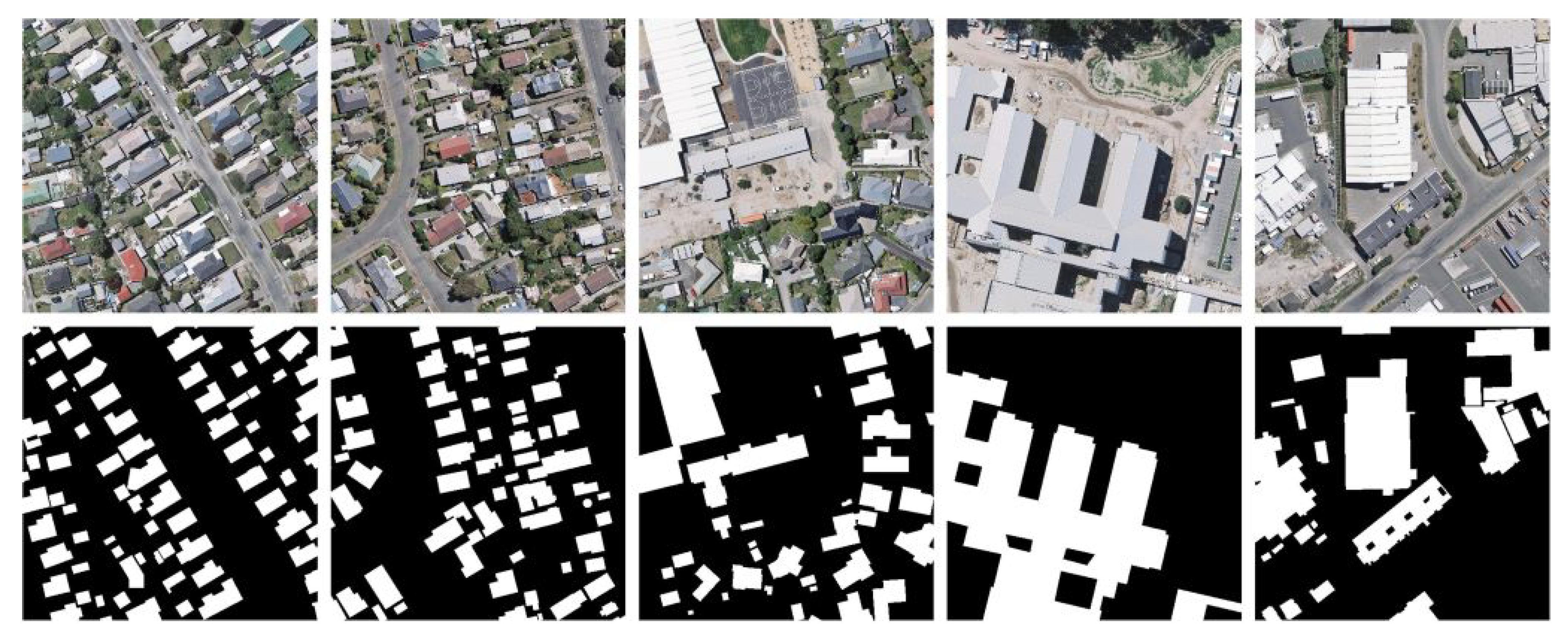
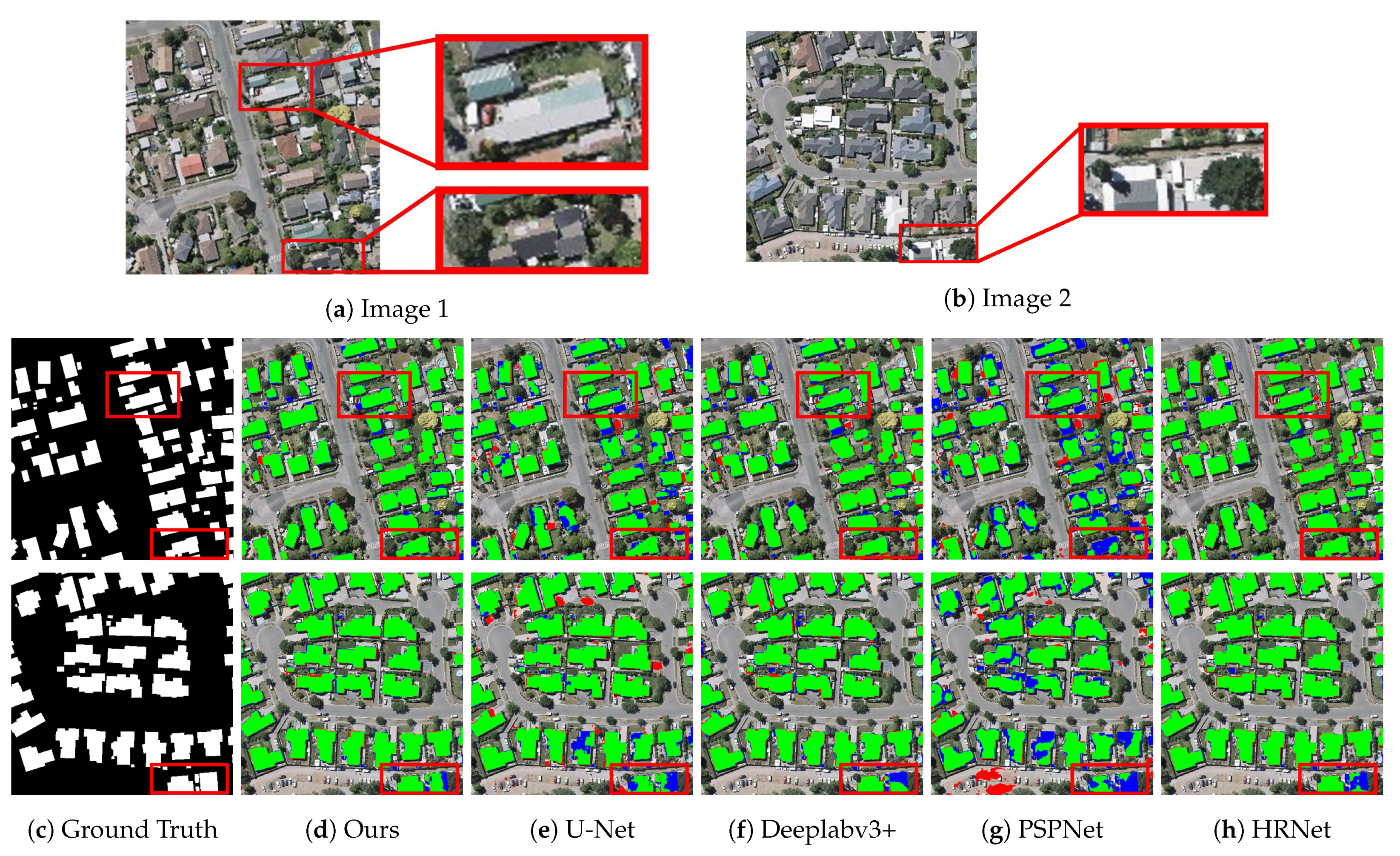
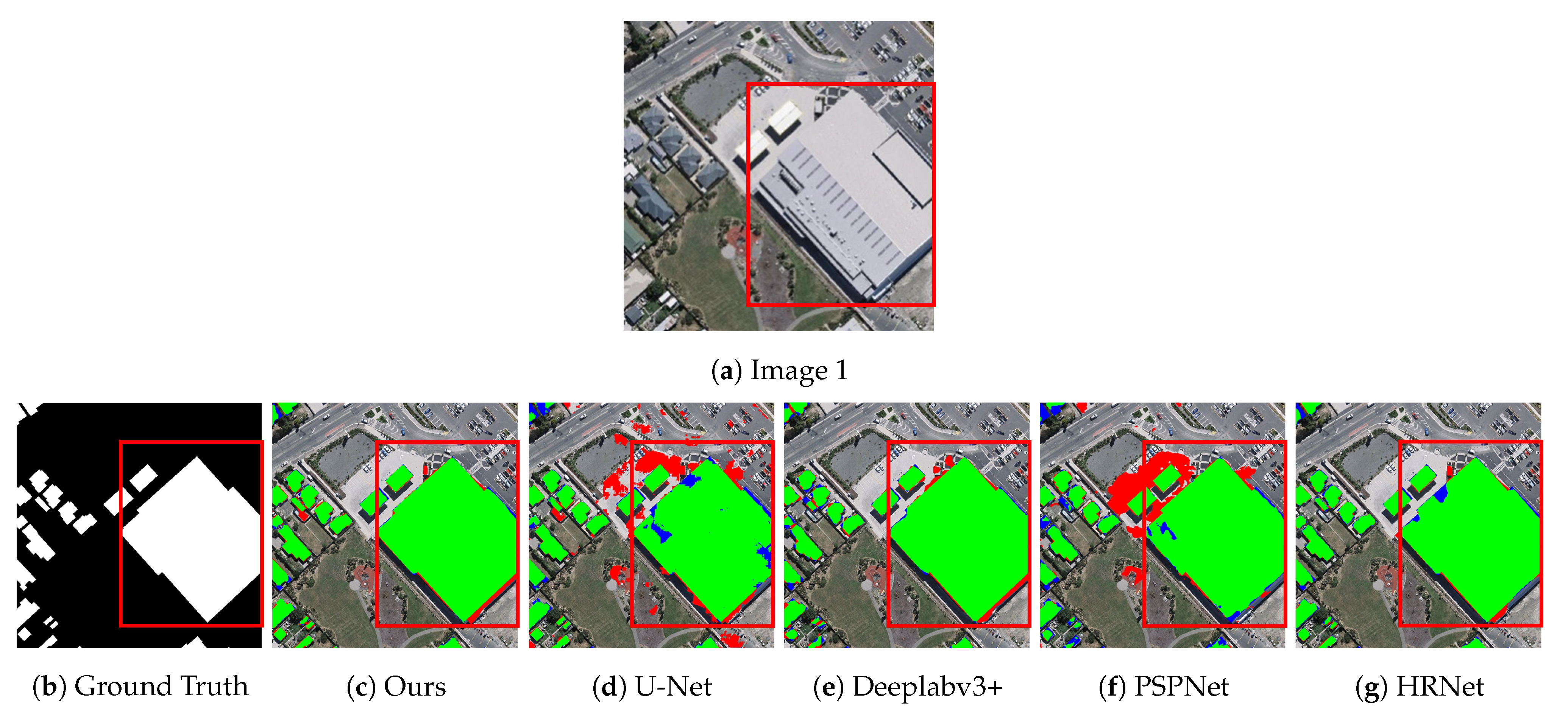
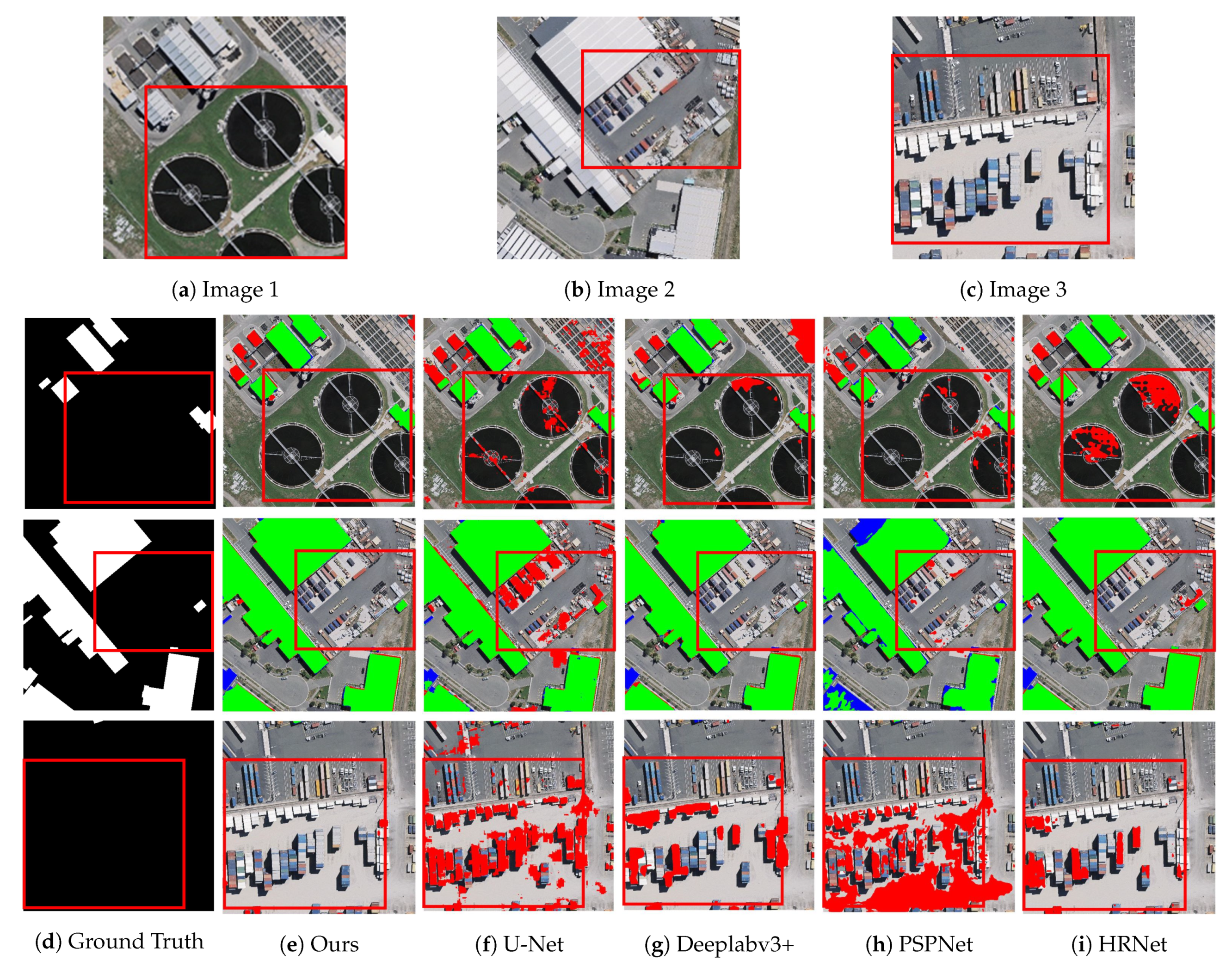
3.3.1. Results on WHU Building Dataset

CFENet is compared with four methods, U-Net [28], Deeplabv3+ [50], PSPNet [30], and HRNet [31]. All these methods have good results in the semantic segmentation task. U-Net started as a semantic segmentation network applied to medical images, and due to its elegant network structure is widely used in semantic segmentation tasks of images in various fields. Deeplabv3+ is based on Deeplabv3, adding a simple and efficient decoder to refine the segmentation results. PSPNet reduces error segmentation by introducing more contextual and multi-scale information. HRNet is used for the representation of high-resolution images, which preserves the high-resolution representation by fusing features from different branches. HRNet has achieved great success in tasks such as semantic segmentation, image-level classification, and object detection. The performance of different methods on the WHU Building Dataset is shown in

Table 1. Performance of different methods on the WHU Building Dataset.

Method	PA	PC	F1	IoU	FWIoU
U-Net [28]	0.9713	0.8366	0.8435	0.7419	0.9485
Deeplabv3+ [50]	0.9816	0.9001	0.9010	0.8296	0.9651
PSPNet [30]	0.9586	0.8215	0.7734	0.6434	0.9247
HRNet [31]	0.9864	0.9109	0.9201	0.8647	0.9742
CFENet (Ours)	0.9871	0.9370	0.9262	0.8722	0.9751

. Our method outperforms other methods on all five evaluation metrics. In particular, our method improves 0.0158 on PA, 0.1004 on PC, 0.0827 on F1, 0.0266 on FWIoU and even more on IoU by 0.1303 over U-Net which is currently used mainly for building extraction tasks. The experimental results of CFENet also show some improvement over HRNet which excels in semantic segmentation, especially the PC improvement of 0.0261.

We qualitatively assess the building extraction results of different methods on the WHU Building Dataset. In the visualization, green areas represent building pixels that are correctly predicted, red areas represent pixels that are actually background but incorrectly predicted as buildings, and blue areas represent pixels that are actually buildings but incorrectly predicted as background. As shown in Figure 5, our method shows better performance in dealing with small-sized and complex-shaped buildings, whereas the other four methods show more or less prediction bias. The buildings in the first row of Figure 6 are large buildings with rich textures and colors. Our method can extract buildings with richer details. The other four methods have the problem that the details of the extraction results are not prominent when extracting such buildings. The cistern shown in Figure 7a has a ground texture that is highly similar to the building footprint. Figure 7b,c are some containers where the surface texture is highly confused with the building. Our method can effectively identify accurate building footprints when dealing with such ground facilities that are easily confused with buildings, while the other four methods suffer from misidentification. Therefore, our method effectively solves the problems of inaccurate extraction results and insufficient detail of extracted buildings when extracting complex buildings.

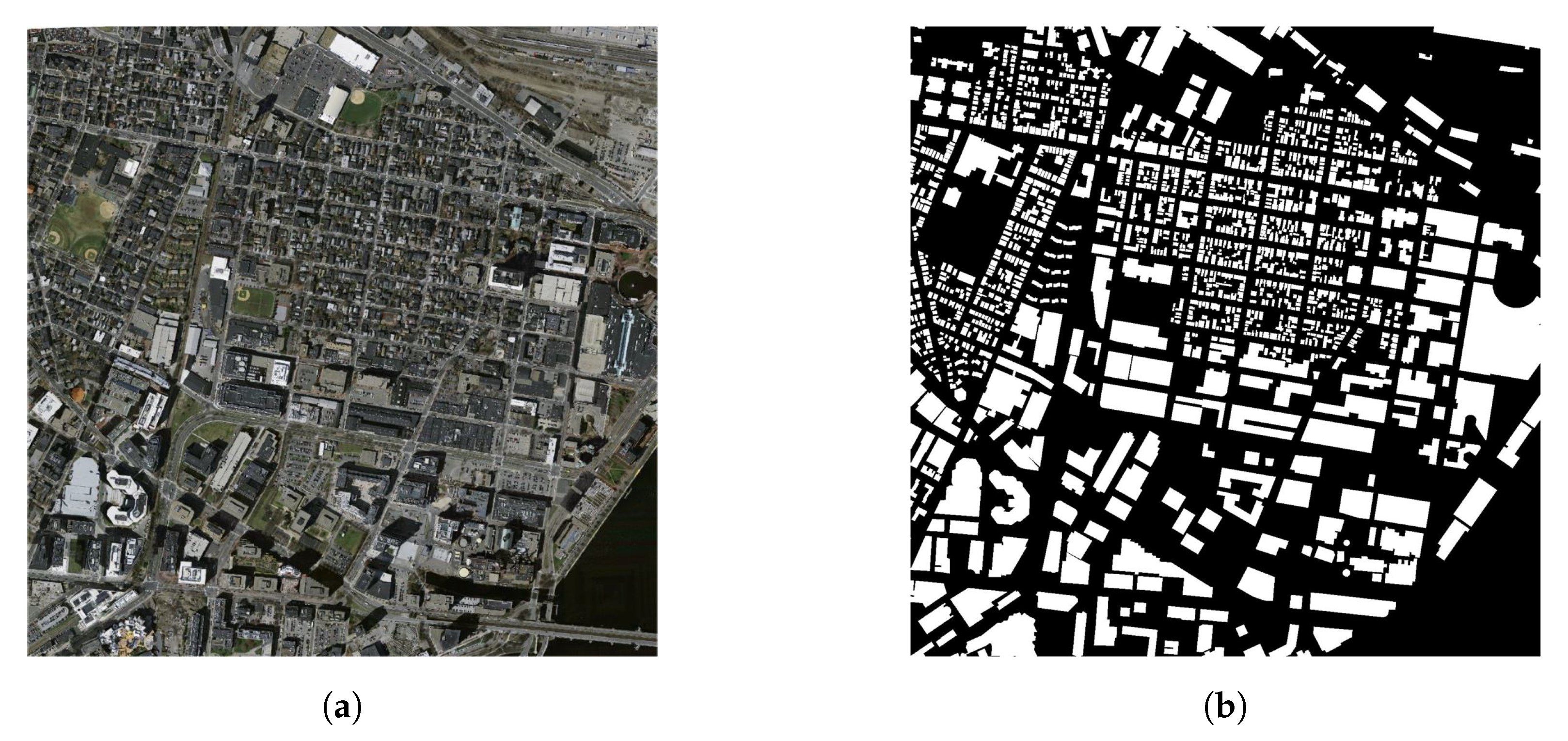
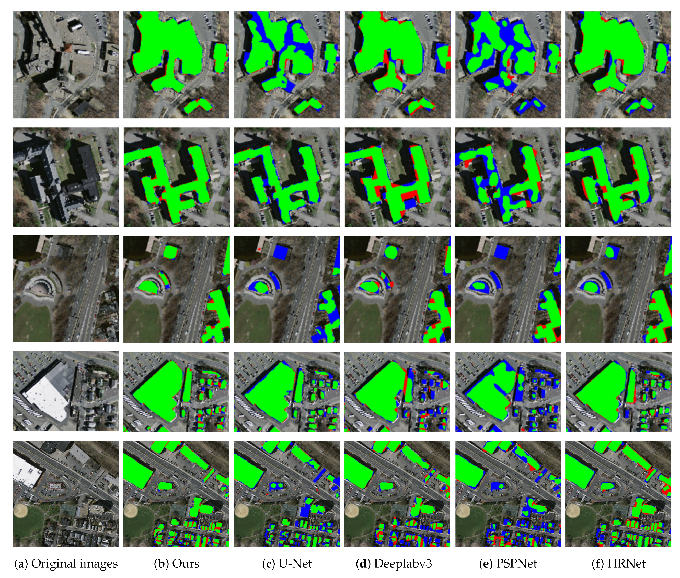
3.3.2. Results on Massachusetts Building Dataset

We conduct experiments on the Massachusetts Buildings Dataset to further validate the effectiveness of CFENet. The experimental results of different methods on the Massachusetts Building Dataset are shown in

Table 2. Performance of different methods on the Massachusetts Building Dataset.

Method	PA	PC	F1	IoU	FWIoU
U-Net	0.9517	0.8635	0.7701	0.6626	0.9099
Deeplabv3+	0.9163	0.7153	0.6506	0.5266	0.8559
PSPNet	0.9116	0.7375	0.6084	0.4704	0.8455
HRNet	0.9581	0.8292	0.7910	0.6968	0.9225
CFENet (Ours)	0.9626	0.8277	0.8304	0.7486	0.9317

. Our method also shows impressive performance on all five evaluation metrics. Among them, on IoU, CFENet improves the performance to 0.7486. On PA, our method achieves 0.9626, significantly outperforming the other methods we compared.

The qualitative assessment results on the Massachusetts Building Dataset are shown in Figure 8. The visualization result shows that CFENet has high extraction accuracy, and most of the buildings are predicted as true positives (green). Row 1, 2, and 4 are large, irregularly shaped buildings that other methods misjudge (red and blue) in predicting such buildings. Row 3 is of complex textured buildings, and Row 5 of buildings is small and dense. CFENet is basically accurate in predicting such buildings, whereas other methods predict some false positives (red) and false negatives (blue).

3.4. Ablation Experiments

As shown in

Table 3. Ablation study on WHU Building Dataset.

Method	BaseNet	Component			PA	PC	F1	IoU	FWIoU
		SFM	FEM	FDM
FCN	ResNet-101				0.9638	0.7578	0.8387	0.7309	0.9365
CFENet	ResNet-101	√			0.9806	0.8954	0.8887	0.8148	0.9640
CFENet	ResNet-101	√	√		0.9864	0.9182	0.9161	0.8608	0.9744
CFENet	ResNet-101	√	√	√	0.9871	0.9370	0.9262	0.8722	0.9751

, our proposed three modules significantly improve the performance. Compared with the baseline FCN (ResNet-101), we improve PA/PC/F1/IoU/ FWIoU by 0.0168/0.1376/0.05/0.0839/0.0275 by using only the spatial fusion module. The effect of using both the spatial fusion module and the focus enhance module improved over baseline on all five evaluation metrics. When three modules are integrated together, the PA/PC/F1/IoU/FWIoU of CFENet is further improved to 0.9871/0.9370/0.9262/0.8722/ 0.9751. The experimental results are significantly improved when the three modules we designed are gradually added, proving that our proposed modules are effective. Therefore, our proposed three modules are of great help for building extraction from high-resolution remote sensing images.

The effect of each module is shown in Figure 9. After adding the spatial fusion module to the base network, the boundary of the building is clearer, indicating that the spatial fusion module aggregates the spatial information of low-level features to a great extent. After adding the focus enhancement module on this basis, the details of the building are more prominent, indicating that the focus enhancement module integrates the rich semantic information in the high-level features. The completeness and accuracy of the building are further improved when the three modules are integrated together.

4. Discussion

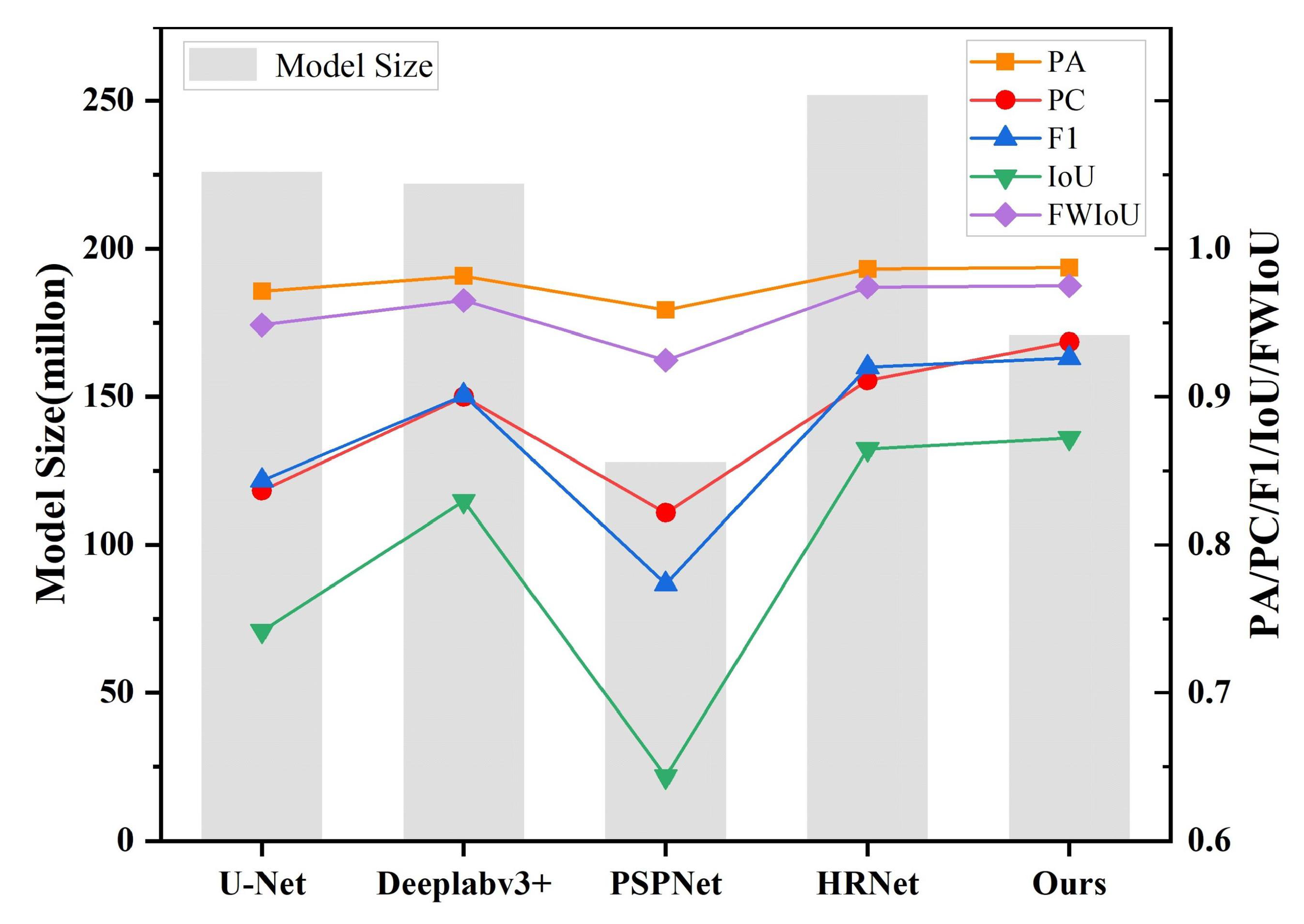
4.1. Comparison of the Efficiency of Different Methods

In addition to the five evaluation metrics mentioned in Section 3.1, we analyze the efficiency of different methods from several aspects under the same batch size. The column “Model Size” represents the total model size for each method. The larger the model, the more memory it takes up during training and testing, and the smaller the model, the faster the model runs. As shown in the column “Model Size” in

Table 4. Comparison of the efficiency of different methods. Different methods are trained on the WHU Building Dataset for 200 epochs, and the batch size is set to 8. The column “Model Size” represents the total model size of each method. The column “Time” represents the time required to train an epoch.

Method	Batch Size	Model Size (Million)	Time (Min/Epoch)
U-Net (ResNet-101)	8	226	20.050
Deeplabv3+ (ResNet-101)	8	222	10.417
PSPNet (ResNet-101)	8	128	20.383
HRNet	8	252	20.450
CFENet (ResNet-101)	8	171	13.250

, the model size of CFENet is only larger than that of PSPNet. Figure 10 shows the model size and the experimental results of different methods on the WHU Building Dataset. Although the model size of CFENet is larger than that of PSPNet, our experimental results are the best among the five methods, and the experimental results of PSPNet are the worst. This indicates that other methods require more memory during training and testing. The reason why CFENet has fewer total parameters is that we use a lot of dilated convolution layers in our network, and use 1 × n convolution layers plus n × 1 convolution layers instead of n × n convolution layers, and use 1 × 1 convolution layers for dimensionality reduction when appropriate. The advantage is that the model size can be reduced, and the performance can also be improved. Therefore, CFENet has a relatively small model to ensure good results.

The column “Time” of Table 4 represents the time required to train an epoch. CFENet takes 13.250 min to train an epoch, which is only slower than Deeplabv3+, and much lower than U-Net, Deeplabv3+, and PSPNet. It is worth mentioning that although the model of PSPNet is smaller than CFENet, PSPNet takes 20.383 min to train an epoch, which is much slower than our method.

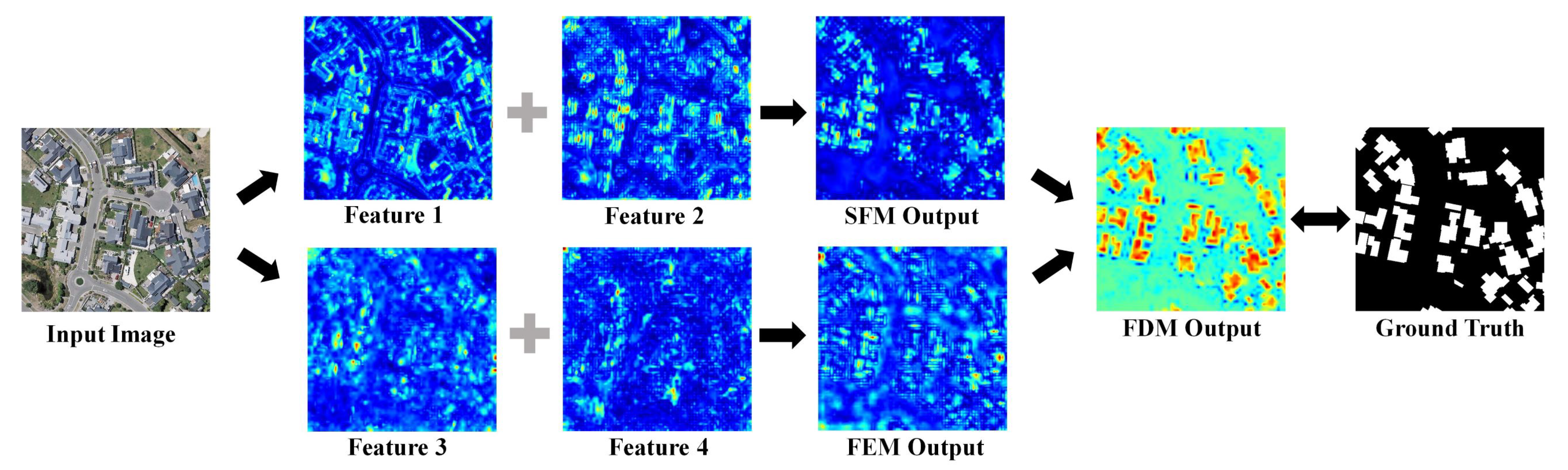
4.2. Heatmaps for Validating the Effectiveness of CFENet’s Modules

To further validate the effectiveness of our proposed modules, we perform a heatmap analysis of the features on the test images. The heatmap visualization of the features is shown in Figure 11. For the low-level features Feature 1 and Feature 2 extracted by ResNet-101, their spatial information is more abundant and leads to information redundancy because they are applied with fewer convolution layers. Therefore, many background pixels in the heatmap appear as highlighted cases. These highlighted background pixels are significantly improved after being processed by the spatial fusion module. The high-level features Feature 3 and Feature 4 extracted by ResNet-101 have more abstract feature information and rich semantic information (categories, attributes, etc.) due to the large number of convolutions. It can be observed from Figure 11 that the features processed by the focus enhancement module are significantly more similar to the ground truth, which proves the effectiveness of the focus enhancement module. The enhanced low-level and high-level features are fed into the feature decoder module for fusion and decoding. The output of the feature decoder module is very close to the ground truth.

5. Conclusions

This paper proposes an end-to-end neural network (CFENet) that can effectively enhance low-level and high-level features and fuse them to obtain strong feature representations for building extraction tasks. Specifically, we introduce the spatial fusion and focus enhancement modules to efficiently enhance the low-level features and high-level features extracted by ResNet-101, respectively. Then the feature decoder module further fuses and enhances the features generated by the spatial fusion module and the focus enhancement module to obtain the final probability map. CFENet achieves superior performance over other methods we have compared on the WHU Building Dataset and the Massachusetts Building Dataset, and significantly improves the extraction accuracy while controlling the computational cost. Moreover, ablation experiments show that our proposed three modules can improve the accuracy of building extraction from remote sensing images.

In future work, our method could be further explored and improved in the following aspects. The generalization ability of each module of CFENet could be further improved. The structure of the loss function could be modified to improve the ability to discriminate difficult samples. The remote sensing images could be preprocessed before being input into our network to further improve the performance of CFENet. Meanwhile, our method would be explored in more application areas, such as side scan sonar remote sensing images, etc.

References

1. Ma, L.; Liu, Y.; Zhang, X.; Ye, Y.; Yin, G.; Johnson, B.A. Deep learning in remote sensing applications: A meta-analysis and review. ISPRS J. Photogramm. Remote Sens. 2019, 152, 166–177. [Google Scholar] [CrossRef]
2. Georganos, S.; Grippa, T.; Vanhuysse, S.; Lennert, M.; Shimoni, M.; Kalogirou, S.; Wolff, E. Less is more: Optimizing classification performance through feature selection in a very-high-resolution remote sensing object-based urban application. GISci. Remote Sens. 2018, 55, 221–242. [Google Scholar] [CrossRef]
3. Yang, H.L.; Yuan, J.; Lunga, D.; Laverdiere, M.; Rose, A.; Bhaduri, B. Building Extraction at Scale Using Convolutional Neural Network: Mapping of the United States. IEEE J. Sel. Top. Appl. Earth Obs. Remote Sens. 2018, 11, 2600–2614. [Google Scholar]
4. Kuras, A.; Brell, M.; Rizzi, J.; Burud, I. Hyperspectral and Lidar Data Applied to the Urban Land Cover Machine Learning and Neural-Network-Based Classification: A Review. Remote Sens. 2021, 13, 3393. [Google Scholar] [CrossRef]
5. Munawar, H.S.; Ullah, F.; Qayyum, S.; Heravi, A. Application of deep learning on uav-based aerial images for flood detection. Smart Cities 2021, 4, 1220–1242. [Google Scholar] [CrossRef]
6. Wang, Y.; Cui, L.; Zhang, C.; Chen, W.; Xu, Y.; Zhang, Q. A Two-Stage Seismic Damage Assessment Method for Small, Dense, and Imbalanced Buildings in Remote Sensing Images. Remote Sens. 2022, 14, 1012. [Google Scholar] [CrossRef]
7. Peng, B.; Ren, D.; Zheng, C.; Lu, A. TRDet: Two-Stage Rotated Detection of Rural Buildings in Remote Sensing Images. Remote Sens. 2022, 14, 522. [Google Scholar] [CrossRef]
8. Mahabir, R.; Croitoru, A.; Crooks, A.T.; Agouris, P.; Stefanidis, A. A critical review of high and very high-resolution remote sensing approaches for detecting and mapping slums: Trends, challenges and emerging opportunities. Urban Sci. 2018, 2, 8. [Google Scholar] [CrossRef] [Green Version]
9. Ball, J.E.; Anderson, D.T.; Chan Sr, C.S. Comprehensive survey of deep learning in remote sensing: Theories, tools, and challenges for the community. J. Appl. Remote Sens. 2017, 11, 042609. [Google Scholar] [CrossRef] [Green Version]
10. Luo, L.; Li, P.; Yan, X. Deep Learning-Based Building Extraction from Remote Sensing Images: A Comprehensive Review. Energies 2021, 14, 7982. [Google Scholar] [CrossRef]
11. Li, E.; Xu, S.; Meng, W.; Zhang, X. Building extraction from remotely sensed images by integrating saliency cue. IEEE J. Sel. Top. Appl. Earth Obs. Remote Sens. 2016, 10, 906–919. [Google Scholar] [CrossRef]
12. Chen, R.; Li, X.; Li, J. Object-Based Features for House Detection from RGB High-Resolution Images. Remote Sens. 2018, 10, 451. [Google Scholar] [CrossRef] [Green Version]
13. Inglada, J. Automatic recognition of man-made objects in high resolution optical remote sensing images by SVM classification of geometric image features. ISPRS J. Photogramm. Remote Sens. 2007, 62, 236–248. [Google Scholar] [CrossRef]
14. Ding, Z.; Wang, X.; Li, Y.; Zhang, S. Study on building extraction from high-resolution images using Mbi. Int. Arch. Photogramm. Remote Sens. Spat. Inf. Sci 2018, 42. [Google Scholar] [CrossRef] [Green Version]
15. Katartzis, A.; Sahli, H.; Nyssen, E.; Cornelis, J. Detection of buildings from a single airborne image using a Markov random field model. In Proceedings of the IGARSS 2001, Scanning the Present and Resolving the Future, IEEE 2001 International Geoscience and Remote Sensing Symposium (Cat. No. 01CH37217), Sydney, NSW, Australia, 9–13 July 2001; Volume 6, pp. 2832–2834. [Google Scholar]
16. Awrangjeb, M.; Fraser, C.S. An automatic and threshold-free performance evaluation system for building extraction techniques from airborne LIDAR data. IEEE J. Sel. Top. Appl. Earth Obs. Remote Sens. 2014, 7, 4184–4198. [Google Scholar] [CrossRef]
17. Tu, Z.; Li, H.; Zhang, D.; Dauwels, J.; Li, B.; Yuan, J. Action-stage emphasized spatiotemporal VLAD for video action recognition. IEEE Trans. Image Process. 2019, 28, 2799–2812. [Google Scholar] [CrossRef]
18. Zhang, D.; He, L.; Tu, Z.; Han, F.; Zhang, S.; Yang, B. Learning motion representation for real-time spatio-temporal action localization. Pattern Recognit. 2020, 103, 107312. [Google Scholar] [CrossRef]
19. Zhang, D.; He, F.; Tu, Z.; Zou, L.; Chen, Y. Pointwise geometric and semantic learning network on 3D point clouds. Integr.-Comput.-Aided Eng. 2020, 27, 57–75. [Google Scholar] [CrossRef]
20. Simonyan, K.; Zisserman, A. Very deep convolutional networks for large-scale image recognition. arXiv 2014, arXiv:1409.1556. [Google Scholar]
21. He, K.; Zhang, X.; Ren, S.; Sun, J. Deep residual learning for image recognition. In Proceedings of the IEEE Conference on Computer Vision and Pattern Recognition, Las Vegas, NV, USA, 27–30 June 2016; pp. 770–778. [Google Scholar]
22. Szegedy, C.; Vanhoucke, V.; Ioffe, S.; Shlens, J.; Wojna, Z. Rethinking the inception architecture for computer vision. In Proceedings of the IEEE Conference on Computer Vision and Pattern Recognition, Las Vegas, NV, USA, 27–30 June 2016; pp. 2818–2826. [Google Scholar]
23. Huang, G.; Liu, Z.; Van Der Maaten, L.; Weinberger, K.Q. Densely connected convolutional networks. In Proceedings of the IEEE Conference on Computer Vision and Pattern Recognition, Honolulu, HI, USA, 21–26 July 2017; pp. 4700–4708. [Google Scholar]
24. Krizhevsky, A.; Sutskever, I.; Hinton, G.E. Imagenet classification with deep convolutional neural networks. Adv. Neural Inf. Process. Syst. 2012, 25, 1097–1105. [Google Scholar] [CrossRef]
25. Long, J.; Shelhamer, E.; Darrell, T. Fully convolutional networks for semantic segmentation. In Proceedings of the IEEE Conference on Computer Vision and Pattern Recognition, Boston, MA, USA, 7–12 June 2015; pp. 3431–3440. [Google Scholar]
26. Badrinarayanan, V.; Kendall, A.; SegNet, R.C. A deep convolutional encoder-decoder architecture for image segmentation. arXiv 2015, arXiv:1511.00561. [Google Scholar] [CrossRef] [PubMed]
27. Zeiler, M.D.; Fergus, R. Visualizing and understanding convolutional networks. In Proceedings of the European Conference on Computer Vision, Zurich, Switzerland, 6–12 September 2014; pp. 818–833. [Google Scholar]
28. Ronneberger, O.; Fischer, P.; Brox, T. U-net: Convolutional networks for biomedical image segmentation. In Proceedings of the International Conference on Medical Image Computing and Computer-Assisted Intervention, Munich, Germany, 5–9 October 2015; pp. 234–241. [Google Scholar]
29. Chen, L.C.; Papandreou, G.; Kokkinos, I.; Murphy, K.; Yuille, A.L. Deeplab: Semantic image segmentation with deep convolutional nets, atrous convolution, and fully connected crfs. IEEE Trans. Pattern Anal. Mach. Intell. 2017, 40, 834–848. [Google Scholar] [CrossRef] [PubMed] [Green Version]
30. Zhao, H.; Shi, J.; Qi, X.; Wang, X.; Jia, J. Pyramid scene parsing network. In Proceedings of the IEEE Conference on Computer Vision and Pattern Recognition, Honolulu, HI, USA, 21–26 July 2017; pp. 2881–2890. [Google Scholar]
31. Sun, K.; Xiao, B.; Liu, D.; Wang, J. Deep high-resolution representation learning for human pose estimation. In Proceedings of the IEEE/CVF Conference on Computer Vision and Pattern Recognition, Long Beach, CA, USA, 15–20 June 2019; pp. 5693–5703. [Google Scholar]
32. Guo, M.; Liu, H.; Xu, Y.; Huang, Y. Building extraction based on U-Net with an attention block and multiple losses. Remote Sens. 2020, 12, 1400. [Google Scholar] [CrossRef]
33. Chen, M.; Wu, J.; Liu, L.; Zhao, W.; Tian, F.; Shen, Q.; Zhao, B.; Du, R. DR-Net: An improved network for building extraction from high resolution remote sensing image. Remote Sens. 2021, 13, 294. [Google Scholar] [CrossRef]
34. Shao, Z.; Tang, P.; Wang, Z.; Saleem, N.; Yam, S.; Sommai, C. BRRNet: A fully convolutional neural network for automatic building extraction from high-resolution remote sensing images. Remote Sens. 2020, 12, 1050. [Google Scholar] [CrossRef] [Green Version]
35. Xu, Y.; Wu, L.; Xie, Z.; Chen, Z. Building extraction in very high resolution remote sensing imagery using deep learning and guided filters. Remote Sens. 2018, 10, 144. [Google Scholar] [CrossRef] [Green Version]
36. Zhu, Q.; Liao, C.; Hu, H.; Mei, X.; Li, H. MAP-Net: Multiple Attending Path Neural Network for Building Footprint Extraction from Remote Sensed Imagery. IEEE Trans. Geosci. Remote Sens. 2021, 59, 6169–6181. [Google Scholar] [CrossRef]
37. Liao, C.; Hu, H.; Li, H.; Ge, X.; Chen, M.; Li, C.; Zhu, Q. Joint Learning of Contour and Structure for Boundary-Preserved Building Extraction. Remote Sens. 2021, 13, 1049. [Google Scholar] [CrossRef]
38. Yang, H.; Wu, P.; Yao, X.; Wu, Y.; Wang, B.; Xu, Y. Building extraction in very high resolution imagery by dense-attention networks. Remote Sens. 2018, 10, 1768. [Google Scholar] [CrossRef] [Green Version]
39. Wen, Q.; Jiang, K.; Wang, W.; Liu, Q.; Guo, Q.; Li, L.; Wang, P. Automatic building extraction from Google Earth images under complex backgrounds based on deep instance segmentation network. Sensors 2019, 19, 333. [Google Scholar] [CrossRef] [Green Version]
40. Zheng, G.; Zhang, H.; Li, Y.; Zhao, J. A Universal Automatic Bottom Tracking Method of Side Scan Sonar Data Based on Semantic Segmentation. Remote Sens. 2021, 13, 1945. [Google Scholar] [CrossRef]
41. Yu, Y.; Zhao, J.; Gong, Q.; Huang, C.; Zheng, G.; Ma, J. Real-Time Underwater Maritime Object Detection in Side-Scan Sonar Images Based on Transformer-YOLOv5. Remote Sens. 2021, 13, 3555. [Google Scholar] [CrossRef]
42. Ji, S.; Wei, S.; Lu, M. Fully convolutional networks for multisource building extraction from an open aerial and satellite imagery data set. IEEE Trans. Geosci. Remote Sens. 2018, 57, 574–586. [Google Scholar] [CrossRef]
43. Mnih, V. Machine Learning for Aerial Image Labeling. Ph.D. Thesis, University of Toronto, Toronto, ON, Canada, 2013. [Google Scholar]
44. Yu, F.; Koltun, V. Multi-scale context aggregation by dilated convolutions. arXiv 2015, arXiv:1511.07122. [Google Scholar]
45. Fu, J.; Liu, J.; Tian, H.; Li, Y.; Bao, Y.; Fang, Z.; Lu, H. Dual attention network for scene segmentation. In Proceedings of the IEEE/CVF Conference on Computer Vision and Pattern Recognition, Long Beach, CA, USA, 15–20 June 2019; pp. 3146–3154. [Google Scholar]
46. Hu, J.; Shen, L.; Sun, G. Squeeze-and-excitation networks. In Proceedings of the IEEE Conference on Computer Vision and Pattern Recognition, Salt Lake City, UT, USA, 18–23 June 2018; pp. 7132–7141. [Google Scholar]
47. Denton, E.L.; Zaremba, W.; Bruna, J.; LeCun, Y.; Fergus, R. Exploiting linear structure within convolutional networks for efficient evaluation. Adv. Neural Inf. Process. Syst. 2014, 27, 1269–1277. [Google Scholar]
48. Jaderberg, M.; Vedaldi, A.; Zisserman, A. Speeding up convolutional neural networks with low rank expansions. arXiv 2014, arXiv:1405.3866. [Google Scholar]
49. De Boer, P.T.; Kroese, D.P.; Mannor, S.; Rubinstein, R.Y. A tutorial on the cross-entropy method. Ann. Oper. Res. 2005, 134, 19–67. [Google Scholar] [CrossRef]
50. Chen, L.C.; Zhu, Y.; Papandreou, G.; Schroff, F.; Adam, H. Encoder-decoder with atrous separable convolution for semantic image segmentation. In Proceedings of the European Conference on Computer Vision (ECCV), Munich, Germany, 8–14 September 2018; pp. 801–818. [Google Scholar]
Figure 1. Our network Context Feature Enhancement Network (CFENet) adopts a ResNet-101 as the backbone. It consists of three novel modules: Spatial Fusion Module (SFM), Focus Enhancement Module (FEM), and Feature Decoder Module (FDM). The input image size of our network is 512 × 512 pixels, and the outputs of the four stages of ResNet-101 are used as Feature 1, Feature 2, Feature 3, and Feature 4, respectively. Then Feature 1 and Feature 2 are fed into the SFM, and Feature 3 and Feature 4 are fed into the FEM. Finally, we input the FDM to obtain the final segmentation result. (a) An overall structure of CFENet. (b) Structure diagram of SFM, FEM, and FDM.
Remotesensing 14 02276 g001
Figure 2. The architecture of Location Block.
Remotesensing 14 02276 g002
Figure 3. Some examples of the WHU Building Dataset. The first row is the original image and the second row is the ground truth.
Remotesensing 14 02276 g003
Figure 4. An example of the Massachusetts Building Dataset. (a) Original image; (b) Ground truth.
Remotesensing 14 02276 g004
Figure 5. Results of different methods on buildings of small size and complex shapes. (a,b) are the original images; (c) ground truth; (d) the results of CFENet; (eh) show the results of U-Net, Deeplabv3+, PSPNet and HRNet, respectively. Green, red, and blue pixels on the map represent predictions of true positives, false positives, and false negatives, respectively. The experimental results in the red box show the areas where the contrast effect is more obvious.
Remotesensing 14 02276 g005
Figure 6. Results of different methods on large buildings with complex textures and colors. (a) Original image; (b) ground truth; (c) the results of our CFENet; (dg) show the results of U-Net, Deeplabv3+, PSPNet, and HRNet, respectively. Green, red, and blue pixels on the map represent predictions of true positives, false positives, and false negatives, respectively. The experimental results in the red box show the areas where the contrast effect is more obvious.
Remotesensing 14 02276 g006
Figure 7. Results of different methods on easily confused buildings. (ac) Original input images; (d) ground truth; (ei) the results of our method and the other four methods, respectively. Green, red, and blue pixels on the map represent predictions of true positives, false positives, and false negatives, respectively. The experimental results in the red box show the areas where the contrast effect is more obvious.
Remotesensing 14 02276 g007
Figure 8. Extraction results of different methods for different types of buildings on the Massachusetts Building Dataset. (a) Original input image; (bf) the results of our method and the other four methods, respectively. Green, red, and blue pixels on the map represent predictions of true positives, false positives, and false negatives, respectively.
Remotesensing 14 02276 g008
Figure 9. Visualization results of ablation experiments. (a) Original image; (b) the output of BaseNet (ResNet-101); (c) the output of BaseNet + SFM; (d) the output of BaseNet + SFM + FEM; (e) the output of CFENet (BaseNet + SFM + FEM + FDM); (f) ground truth. The experimental results in the box show areas where the contrast effect is more obvious.
Remotesensing 14 02276 g009
Figure 10. Comparison of experimental results and model sizes of different methods. Line graphs with different colors represent the results of different evaluation metrics. The histogram represents the model sizes of different methods.
Remotesensing 14 02276 g010
Figure 11. Heatmaps of CFENet’s feature maps. SFM Output represents the feature maps output by the spatial fusion module. FEM Output represents the feature maps output by the focus enhancement module. FDM Output represents the feature maps output by the feature decoder module.
Remotesensing 14 02276 g011