An Integrated Model of Summer and Winter for Chlorophyll-a Retrieval in the Pearl River Estuary Based on Hyperspectral Data

Abstract

Chlorophyll-a (Chla) is an important parameter for water quality. For remote sensing-based methods for the measurement of Chla, in-situ hyperspectral data is crucial for building retrieval models. In the Pearl River Estuary, we used 61 groups of in-situ hyperspectral data and corresponding Chla concentrations collected in July and December 2020 to build a Chla retrieval model that takes the two different seasons and the turbidity of water into consideration. The following results were obtained. (1) Based on the pre-processing techniques for hyperspectral data, it was shown that the first-derivative of 680 nm is the optimal band for the estimation of Chla in the Pearl River Estuary, with R² > 0.8 and MAPE of 26.03%. (2) To overcome the spectral resolution problem in satellite image retrieval, based on the simulated reflectance from the Sentinel-2 satellite and the shape of the discrete spectral curve, we constructed a multispectral model using the slope difference index method, which reached a R² of 0.78 and MAPE of 35.21% and can integrate the summer and winter data. (3) The slope difference method applied to the Sentinel-2 image shows better performance than the red-NIR ratio method. Therefore, the method proposed in this paper is practicable for Chla monitoring of coastal waters based on both in-situ data and images.

1. Introduction

Over the past decades, significant contributions have been made in coastal and inland water quality prediction using remote sensing data. Chlorophyll-a (Chla) is the most abundant pigment in phytoplankton or algae. Chla in water is an important water quality index [1]. Its concentration reflects the condition of eutrophication; it is thus an important indicator for water quality monitoring, despite the challenges in Chla estimation for coastal waters [2,3]. The combination of remote sensing techniques and traditional field monitoring can obtain the distribution and change of water quality in large water bodies in a timely manner. It is a convenient and economical method for long-term dynamic monitoring for large study areas [4,5,6]. Besides, conventional field sampling approaches have difficulty identifying spatial and temporal patterns in water quality. Various models based on remote-sensing techniques have been proposed for different water areas and water quality parameters [7,8]. The current research outputs of remote sensing for water quality can be generally divided into the following three aspects: research objects, modeling methods, and the data used for Chla prediction. These pioneering study outputs indicate the unprecedented potential of applying satellite images for long-term water quality monitoring of inland and coastal water bodies.

The research objects refer to the type of water and its water quality indicators. For the type of water, there are mainly two types: case 1 and case 2 waters [4,9,10]. In the definitions commonly used today, the case 1 waters are those whose combinations of water constituents are relatively simple, being predominantly phytoplankton, such as in most open seas [1], and the water quality retrieval models for case 1 have been well developed. In case 2 waters, the components of water are more complex, including Chla, suspended matter, and colored dissolved organic matter (CDOM), which are the water quality indicators (one of the research objects mentioned above). The latter two components, especially suspended matter, are likely to affect predictions of Chla concentration, which increases the difficulty of Chla modeling [4,10,11,12]. In summary, modeling methods for Chla concentration prediction can be divided into two categories: those based on the empirical and physical properties of the models [7,13,14,15], and those using fluorescence-based methods, such as band models, nonlinear mapping, and physical models based on the band combination characteristics [16,17]. For instance, Shuisen Chen et al. [18] established an improved three-band model, which was initially provided by Giorgio Dall’Olmo [19] for the measurement of Chla for the Pearl River Estuary based on the bands 684 nm, 690 nm, and 718 nm. There is also an Ocean Chlorophyll algorithm (OC) specifically developed for ocean chlorophyll [20], as well as its improved versions [21]. Zuomin Wang et al. [22] utilized a stepwise iteration method and found that the first-derivative model had a higher accuracy for Chla prediction for the Seto Inland Sea, Japan. Qian Cheng et al. [16] compared the red-NIR ratio method, first-derivative method, and three-band method in the coastal areas of Zhejiang, China, and concluded that the three-band mixed band model has better ability in Chla estimation. All these investigations indicated that, under the increasingly complex optical conditions in coastal waters, three-band and even multi-band methods are more stable, and thus could become the main approaches for Chla prediction based on remote-sensing techniques.

The data used in Chla prediction includes spectral data from satellite images or in-situ measured spectral data. However, due to the satellites’ remote observation distance, atmospheric influence, coarse spectral resolution, and other issues, the two spectral series are in fact quite different. There is still much room for researchers to improve the relevance between them. The former builds the model directly based on the reflectance from remote sensing imagery and the water quality parameters [23], while the latter develops models utilizing in-situ hyperspectral data and then applies the models to satellite images [24]. Although many current satellites carry multispectral sensors, their spectral resolution is much lower than the in-situ hyperspectral devices. That necessitates the need to develop a corresponding model to improve the relationship between hyperspectral data and multi-spectral images. In addition, due to incomplete atmospheric correction, the corrected reflectance is still much higher than the in-situ counterpart. Direct application of the hyperspectral model to images may obtain larger retrieval results, with a resultant decline in precision [25]. Suwisa Mahasandana et al. [25] built a model for the Bangpakong River Estuary based on three-band combination. The results showed that the RMSE of the model using hyperspectral data was 1.13 mg/m³ (0.13~7.25 mg/m³); however, when applied to Landsat-5 images, the RMSE increased to 1.6 mg/m³ (0.13~7.25 mg/m³), indicating lower accuracy. Thus, there is still room for researchers to improve the relationship between hyperspectral data and multi-spectral images. With improvement, researchers can apply the models established based on in-situ hyperspectral data to multispectral images to obtain large-scale Chla monitoring.

In addition, improvement is necessitated by the seasonal variations in Chla concentration. Many existing studies have reported that the models show differences in representative bands and model performance. Due to the regional specificity of many models, high accuracy can be validated in one water area, but usually not in another water area [8]. Spectral curves vary in different waters and different seasons, but changes generally fluctuate near representative bands, with band width of 1~10 nm [26,27]. Some researchers have also tried to discuss the seasonal data separately. For instance, K. Kallio et al. [28] developed individual models for May and August separately, using the same band combination for Chla monitoring in southern Finland. Chen Gao [29] selected different seasonal models due to the data discrepancy between August and January. Xing et al. [30] used the ratio method near bands of 700 nm and 670 nm for the spectral data of May and August in the Pearl River Estuary, but obtained a poor fitting effect. In the aforementioned studies, the data from different seasons were modeled separately with varied performance [31]. However, for seasons or months without in-situ hyperspectral data, researchers have been unable to develop appropriate models for such periods; the retrieval accuracy cannot be guaranteed either. A more universal and stable model is required to perform well in different conditions.

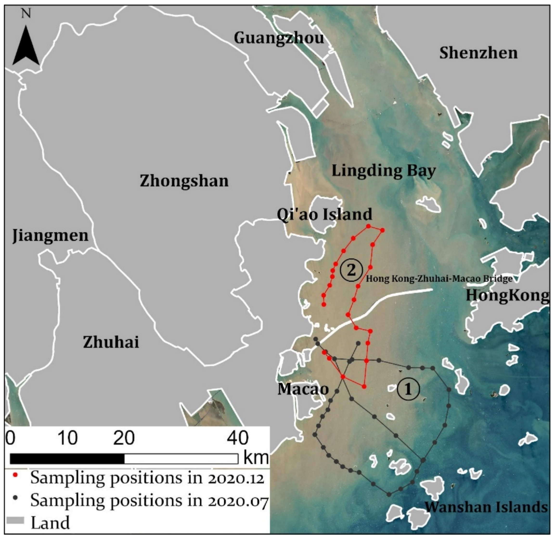
In view of the problems in the above research results, such as applying the in-situ hyperspectral model to multi-spectral image, and the problem that waters in different areas and seasons cannot be modeled in an integrated manner, this paper makes some proposals. In this study, we used the Pearl River Estuary (PRE) as the study area aiming to propose a more universal and stable model for Chlorophyll-a retrieval. The model can achieve satisfactory performance for different seasonal hyperspectral data. Finally, the proposed model can also be applied to multispectral images to perform large-scale applications.

2. Materials and Methods

2.1. Study Area

The study area is located in the South China Sea near the Pearl River Estuary (PRE) in Guangdong Province, China. The study area is a transition region between the Pearl River Estuary and the South China Sea, from Qi’ao Island in the north and Wanshan Islands in the south. It covers some crucial landmark regions, such as the Hong Kong-Zhuhai-Macao Bridge, the Wanshan Islands, and Lingding Bay.

Figure 1 shows the map of the study area and its surroundings, and the spatial distribution of the sampling sites for the two-round field sampling. During sampling, a sample was taken for every 15 min the boat traveled. For each sampling, the environment factors, such as the wind speed, the travel speed of the boat, and the distance of sampling positions were not all the same. PRE is close to the Pearl River Delta, one of China’s economically developed areas with dense human activities and complex anthropogenic conditions, leading to optical component complexity of surface waters in this region [32,33], and its spectrum is more affected by the suspended solids.

2.2. Field Data Collection

Field data were collected at the above sampling sites in the PRE on 22 July and 23 July in summer and 20 December in winter, when the Sentinel-2 satellites were passing through the study area. Data collection mainly contained three parts: spectrum, water samples, and other water quality parameter measurement.

The hyperspectral data was measured by the Analytical Spectral Devices (ASD) FieldSpec 4, manufactured by the ASD Company (USA), on the basis of above-water hyperspectral remote sensing reflectance ($R_{rs}$) from NASA-recommended protocols [34]. For each measurement, upward radiance ($L_u$), downward sky radiance ($L_{sky}$), and radiance from the white reference panel (the gray panel for water measurement) ($L_{panel}$) were measured. R_rs was then derived by the equation below:

$$R_{rs}=\frac{{\rho }_{panel}\left(L_u-{\rho }_f\ast L_{sky}\right)}{\pi L_{panel}}$$

(1)

where ${\rho }_{panel}$ is the reflectance of the reference panel (provided by the manufacture) and ${\rho }_f$ is the Fresnel reflectance of the water surface.

Meanwhile, two bottles of 500 mL water were taken at each sampling position for later laboratory analysis for Chla and suspended solids concentration. The water samples were immediately kept in a mobile fridge in a dark place. Other water quality parameters, such as dissolved oxygen, water temperature, pH, etc., were measured by portable hand-held analyzers as well. Salinity was measured in the field by salinometer. Supplementary environmental information, such as longitude, latitude, wind speed, and other special environmental factors, were recorded for subsequent data processing, such as matching the Fresnel reflectance of the water surface for R_rs calculation [35].

In the laboratory, the concentration of Chla was determined by the acetone method with a spectrophotometer [36], and that of suspended solids by the weighted method [37]. The results are shown in the

Table 1. The statistical range, mean, and median values of Chla and suspended solids concentration.

Parameter	Time	Range	Mean Value	Median Value
Chla (mg/m3)	2020.07	3.995~27.312	12.84	10.73
	2020.12	1.527~4.168	2.27	2.08
Suspended solids (mg/L)	2020.07	0.33~54	24.28	24.33
	2020.12	25.2~278	112.31	84.60

.

The initial results showed that environmental conditions such as water temperature in summer were favorable for the growth of phytoplankton. The concentration of Chla was thus very different. In December, Chla was relatively low, as fewer phytoplankton could survive on the surface of the sea.

2.3. Data Pre-Processing and Models

2.3.1. Normalization Processing

Normalization is done to reduce the influence of environment and measurement angle changes [37], and also to avoid noise generated by other environmental interferences on the spectral curve. This allows the quick determination of the wavelength position of the bending point and the peaks of the spectral curve, and reflects the bands with obvious characteristics of parameter indexes in order to facilitate the comparison of data from different positions.

$$R_N\left({\lambda }_i\right)=\frac{R\left({\lambda }_i\right)}{\frac{i}{n}{\displaystyle {\sum }_{i=350}^{900}}R\left({\lambda }_i\right)}$$

(2)

In the formula, $R_N\left({\lambda }_i\right)$ is the normalized reflectance; $R\left({\lambda }_i\right)$ is original reflectance; n is the number of bands from 350 nm to 950 nm. To perform normalization processing, the original spectral reflectance at each position is divided by the corresponding normalized value, thereby obtaining the normalized spectral curves. In this study, the average reflectance between 350~900 nm was selected as the normalized denominator, because this band range covers the most of the water spectrum information. After 900 nm, the reflectance is almost zero due to the absorption of water.

2.3.2. First-Derivate Processing

Using first-derivate processing [38], water spectral reflectance can be mathematically simulated. Different derivate orders can be calculated to determine the bending point of the curve and the location of the maximum value of reflectance, which can be used for calculating the slope or the rate of the change of the reflectance at a certain wavelength. The spectral absorption characteristics such as wavelength position, depth and width can be determined in the water spectrum. First-derivate processing can remove part of the influence of linearity and noise on the target spectrum. The following formula was used for the calculation of first-derivate in this study:

$$R\left({\lambda }_i\right)=\frac{R\left({\lambda }_{i+1}\right)-R\left({\lambda }_{i-1}\right)}{{\lambda }_{i+1}-{\lambda }_{i-1}}$$

(3)

where ${\lambda }_{i+1}$, ${\lambda }_i$, ${\lambda }_{i-1}$ refer to adjacent wavelengths, $R\left({\lambda }_i\right)$ is the first-derivate value at ${\lambda }_i$, $R\left({\lambda }_{i+1}\right),$ and $R\left({\lambda }_{i-1}\right)$ are the original reflectance. If the results of the first-derivate are calculated again, one obtains the second-derivate. The function of the spectral derivative calculation is provided in the Spectral Math module of ENVI 5.3. To reduce the workload, the spectral data is converted into a spectral file that can be read by the software and imported into the calculation to obtain the results.

2.3.3. Equivalent Reflectance Simulation

Sensors carried by different satellites have their unique spectral response functions, which can be understood as a function of the proportion of signals received within the specific band range of a central wavelength of the sensor. Resampling the ground spectrum using this function is equivalent to directly measuring the reflectance on the ground with sensors on the satellites. Based on the spectral response function, the convolution method was applied to the ASD spectral field data to calculate the equivalent reflectance of water corresponding to bands of the satellite sensor [39]. The equation is as follows:

$$R_i=\frac{{\displaystyle {\int }_{{\lambda }_1}^{{\lambda }_2}}{S}_i\left(\lambda \right)R\left(\lambda \right)d\lambda }{{\displaystyle {\int }_{{\lambda }_1}^{{\lambda }_2}}{S}_i\left(\lambda \right)d\lambda }$$

(4)

where $R_i$ denotes the equivalent reflectance of the $i$th band of Sentinel-2, ${\lambda }_1$ to ${\lambda }_2$ is the spectral wavelength range of the $i$th band of Sentinel-2, $R\left(\lambda \right)$ is the corresponding reflectance at wavelength $\lambda$, and $S_i\left(\lambda \right)$ is the corresponding response value of the spectral response function of the $i$th band of Sentinel-2 at wavelength $\lambda$. This calculation can be performed by the spectral resampling tool in the ENVI 5.3 toolbox.

2.3.4. The Slope Difference Index

On basis of the analysis in Section 3.4, this paper used a slope difference index to calculate the slope as the independent variable of the model. The formula is as follow:

$$\{\begin{array}{c}\begin{array}{c}k1=\frac{R\left(B5\right)-R\left(B4\right)}{\lambda \left(B5\right)-\lambda \left(B4\right)}\\ k2=\frac{R\left(B4\right)-R\left(B3\right)}{\lambda \left(B4\right)-\lambda \left(B3\right)}\\ x=k1-k2\end{array}\end{array}$$

(5)

where R is the original reflectance of the corresponding band, λ is the central wavelength (μm) of the corresponding band, k1 is the slope between B5 and B4, k2 is the slope between B4 and B3, and the independent variable x is the difference between these two slopes. In addition, the construction of this method follows the idea of the second-order differential. k1 and k2 can be regarded as the first-order differential of a certain point between B5 and B4, B3, and B4, respectively, and the second-order differential is the difference of the two first-order differentials divided by the band difference, which is the denominator of the slope difference in this paper. As a result, in fact, the two methods differ by a multiplier factor. However, by contrast, the model obtained by the second-derivate value of B4 in the traditional way is not as effective as the proposed slope difference method in this study.

2.3.5. Model Validation and Evaluation

In this paper, one-third of the data was retained for accuracy verification. Root Mean Square Error (RMSE), Mean Absolute Percentage Error (MAPE), and Mean Absolute Error (MAE) [31] were used to evaluate the accuracy. The larger the value, the larger the estimation error and the lower the accuracy of the model.

$$\mathrm{RMSE}=\sqrt{\frac{{\displaystyle {\sum }_{i=1}^n}{\left(C_{iEst}-C_{iAct}\right)}^2}{n}}$$

(6)

$$\mathrm{MAPE}=\frac{{\displaystyle {\sum }_{i=1}^n}\left|\frac{C_{iEst}-C_{iAct}}{C_{iAct}}\right|}{n}\times 100\%$$

(7)

$$\mathrm{MAE}=\frac{{\displaystyle {\sum }_{i=1}^n}\left|C_{iEst}-C_{iAct}\right|}{n}$$

(8)

where, $C_{iEst}$ is the estimated Chla concentration by the model and $C_{iAct}$ is the in-situ measured Chla concentration. According to the above design, two-thirds of the samples were selected for model building, and one-third of the samples for verification, among which 13 samples were picked from the data of July and 7 were obtained in December.

Figure 2 shows the technical roadmap and an overview of the methods applied in this study.

3. Results

3.1. In-Situ Spectral Characteristics

After normalization by Formula (2), the spectral curve tends to be more concentrated (Figure 3b,d), which effectively eliminates the influence of environmental factors during field measurement. It can be seen that the spectral curves in both winter and summer have evident characteristics in reflection and absorption, but the details for fluctuation and smoothness of the curves are different in some representative bands.

Spectral data in the same study area in different periods have obvious seasonal characteristics. Spectral data collected by Yunlin Zhang et al. [40] and Hubert Loisel et al. [41] in different seasons indicated this conclusion as well.

In July, the water was characterized by high Chla concentration, and an absorption valley was formed near the blue-green bands of 500 nm because of the strong absorption of light energy by Chla and yellow substances (CDOM) within this range. A reflection peak was formed near green bands of 550 nm, which can be used as a quantitative indicator of Chla concentration. In the range of 600~700 nm, the absorption of Chla was quite typical and the suspended solids concentration was low, which has little effect on the reflectance uplift as the suspended solids reflection is formed near 800 nm. In the range of 730~900 nm, the reflectance tended to be 0 due to the strong absorption of Chla and water.

In December, the water was characterized by a high suspended solids concentration and a high reflectance on the whole, but the reflectance signature of Chla was not completely covered. A reflection peak was formed near 550 nm of green bands. In the range of 600~700 nm, a wide reflectance plateau was formed due to the dominant effect of suspended solids, followed by a typical infrared absorption valley near 730 nm and a small reflectance peak near 800 nm.

3.2. Model of Normalized Reflectance

3.2.1. Correlation between Normalized Results and Chla

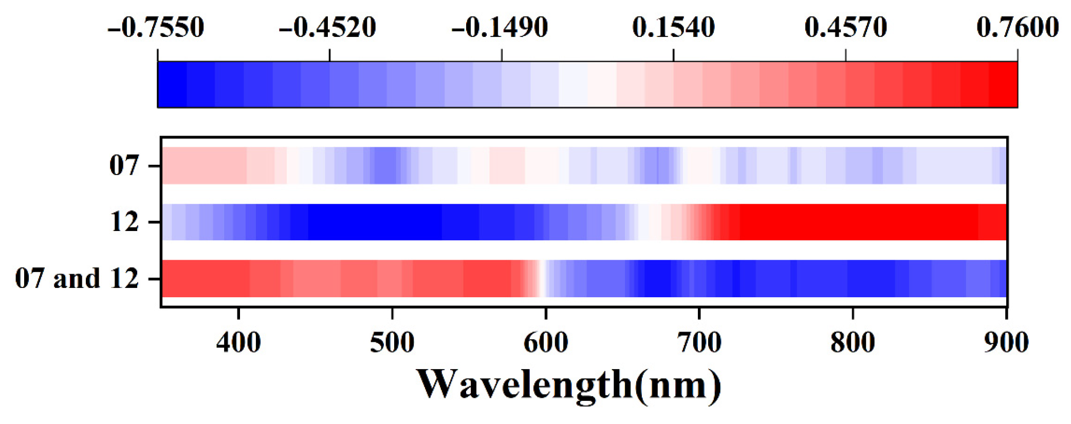
Due to the seasonal differences in spectral curves, the reflection peak, absorption valley, and sensitive bands also changed accordingly, leading to differences in correlation between the normalized difference and Chla concentration. After normalization, the correlation coefficients between Chla concentration and normalized reflectance are enhanced, and compared in Figure 4.

In July, the maximum correlation coefficient between them was −0.39 at 496 nm, which is still weak. In December, the maximum negative correlation was −0.75 at 489 nm and the maximum positive correlation was 0.759 at 827 nm. After combination, compared with the origin reflectance, the positive correlation of the green bands was improved; the maximum positive correlation reached 0.549 at 563 nm and the maximum negative correlation reached −0.691 at 673 nm.

The differences between the two datasets may be attributed to Chla seasonal fluctuation and a difference in the suspended solids concentration. In summer, the concentration of Chla is higher and the spectral characteristics are mainly regulated by it. The highest correlation band (496 nm) appears near the green band, which is one of the characteristic bands of Chla. In winter, the water is not suitable for the survival of phytoplankton, causing low Chla concentration; the spectral characteristics are therefore mainly controlled by suspended solids. Specifically, due to the strong scattering of suspended matter, the correlation of the infrared band (827 nm) may be dominated by suspended matter rather than Chla. This indicates that it is difficult to obtain an integrated model through a simple combination of in-situ measured spectra and Chla concentration collected in different periods [37].

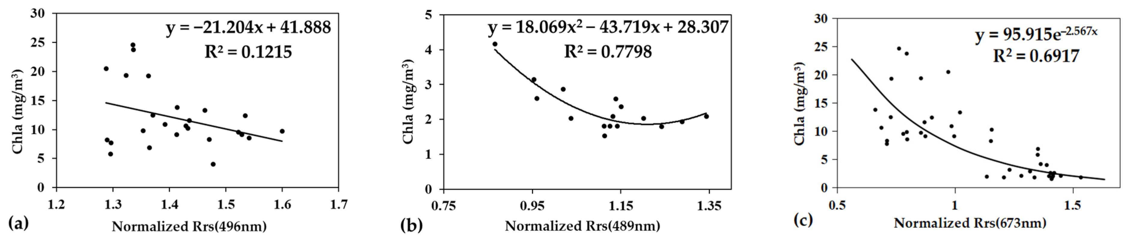
3.2.2. Established Single Band Model for Comparison

According to the correlation analysis between Chla and normalized reflectance, the bands with better correlation were selected for single-band regression analysis.

In Figure 5, the single-band model for July displayed just a weak trend and the high dispersion leads to a quite low R² value, which is not significantly different from the original spectral model, indicating that the transformation of reflectance alone cannot reach an ideal fitting result based on data collected in July. Previous studies also showed that it is difficult to retrieve Chla data in summer [26,29].

The model for December can obtain satisfactory results using only a single band. For the dataset collected in December, the model’s overall R² value is 0.7798. It can be seen that the correlation based on the normalized reflectance has been improved, indicating that the normalization of the original spectrum is conducive to improving model accuracy, but the effect varied dramatically with seasons. Moreover, because the Pearson correlation coefficient represents the linear correlation between two variables, the regression model obtained from the band with the highest correlation coefficient may not necessarily be the most appropriate for the data in July. It was found from the scatter diagram that there is an obvious linear relationship between converted reflectance and Chla concentration, so it is necessary to process and transform the original reflectance and the Chla concentration to obtain a linear relationship for the converted data [42]. Next, we tried to transform the Chla concentration data and took its reciprocal as the dependent variable, namely 1 divided by Chla.

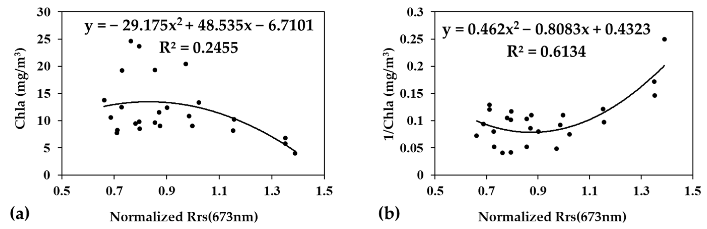
As shown in Figure 6, after the step-by-step iteration, it was found that the unary quadratic model near 673 nm obtained the best fitting result. When the reciprocal of Chla concentration was taken as the dependent variable, the R² increased from 0.24 to above 0.61. Meanwhile, this band was also the one with the highest overall correlation for the datasets of both July and December, which means that the reciprocal method worked for the improvement of model accuracy. Therefore, in order to find more suitable bands and better fitting result, it is necessary to make several attempts and comparisons for different band combinations. After data transformation, the gap between the data can be narrowed to make the data more centralized, which is conducive to modeling, and better correlation superior to single data is obtained.

In addition, the method, called reflectance peak positioning, is commonly used for in-situ measured spectra modeling. After investigation, the reflectance peak for December data was found at 670 nm; this is possibly due to low Chla concentration with a weak effect on the reflectance peak. The variation in Chla concentration in July is larger and the reflectance peak is discrete, leading to a low R² value of approximately 0.2. These results suggested that reflectance peak positioning was not a good option for model improvement in this study. The major cause could be the small range of Chla concentrations; if data with larger ranges are input, better correlation could be obtained.

3.2.3. Established Ratio Model for Comparison

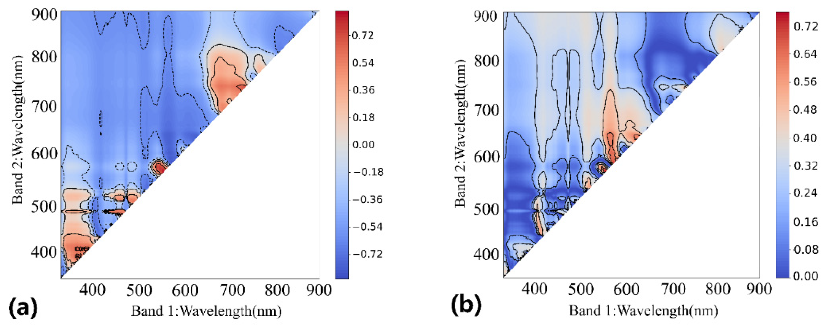
To find the best band ratio combination, we used Python and its libraries (numpy, pandas, matplotlib, etc.) to test the correlation coefficient of all hyperspectral bands.

The regions with the highest correlation coefficient or R² are shown in Figure 7. In Figure 7a, the darker blue or red indicates the higher correlation. In Figure 7b, the darker red indicates the larger R². These are concentrated at the narrow green band (550–690 nm) and at the wide red band (600–700 nm). We picked band pairs at the center of the dark area with the highest R², and plotted their fitting models as follows.

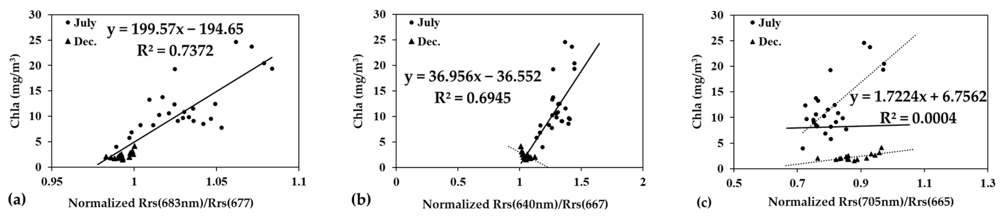
In Figure 8a, the model performs fairly well for the datasets of both July and December and the two datasets have the same trend. However, the two bands’ spectral distance is quite short, with a gap of only 6 nm (683 nm–677 nm), which is suitable for hyperspectral modeling, but it is difficult to obtain two similar bands from commonly-used multi-spectral sensors. When the spectral distance was adjusted to be larger (Figure 8b), the value of R² decreased accordingly. Other band combinations such as normalized R_rs (705)/R_rs (665) (Figure 8c) [15,43] were also tested, but poor correlation was obtained. Yuji Sakuno et al. also found that it is difficult to obtain a universal and stable model for these two datasets collected in different seasons and with different turbidity and Chla concentration [44].

The normalization of the original reflectance is an option to integrate the spectral data collected in different seasons. The correlation coefficient between the normalized spectral value and Chla is better than that based on the original spectrum. The representative bands are somewhat changed, but the correlation is stronger. The ratio model based on normalized data can obtain better correlation than a single-band model, as shown in Figure 5c. However, the data for December showed no obvious trend in that model. In addition to the normalization, the first-derivate processing method was more capable of further exploring the hidden information in the spectrum.

3.3. First-Derivate Model Exploration

The above issue could be related to the water’s optical conditions in the two seasons. The environmental information for the two seasons is different, and the correlation between Chla and original spectral reflectance is not evident; therefore, the data cannot be easily integrated. To solve this problem, derivate processing was employed to eliminate the influence of environment properties, manual measurement error, and suspended solids, so that the concentration of Chla creates a sensitive response in the change rate of reflectance, instead of in the reflectance itself [38,45].

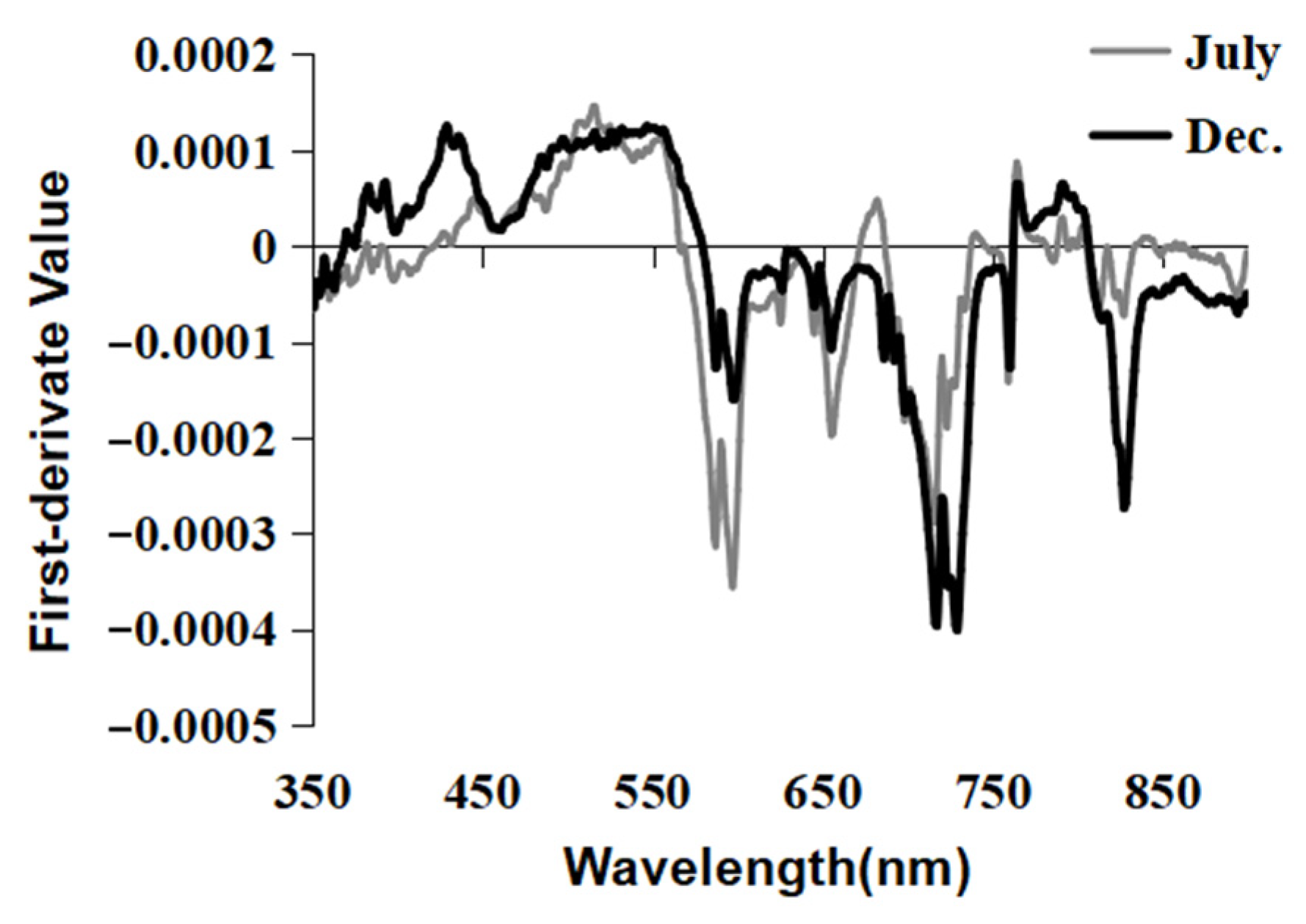
After the first-derivate processing by Formula (3), the spectral curve was graphed by taking the average value for each monthly dataset. In Figure 9, it can be seen that the curve at the peak and bottom values were more obvious. The derivate curves of these two stages tended to create more consistent model construction. The first-derivate curve further emphasized several reflectance variation features. In July, the concentration of Chla was high and the original spectral peak features were extremely narrow and sharp. In December, the original peak features were relatively wide. The reflectance did not change significantly before 680 nm. The reflectance of both datasets changed rapidly at about 600 nm, 650 nm, 680 nm, 710 nm, and 840 nm. Therefore, first-derivate processing can explore the common features between the two datasets and has great advantages in integrated modeling.

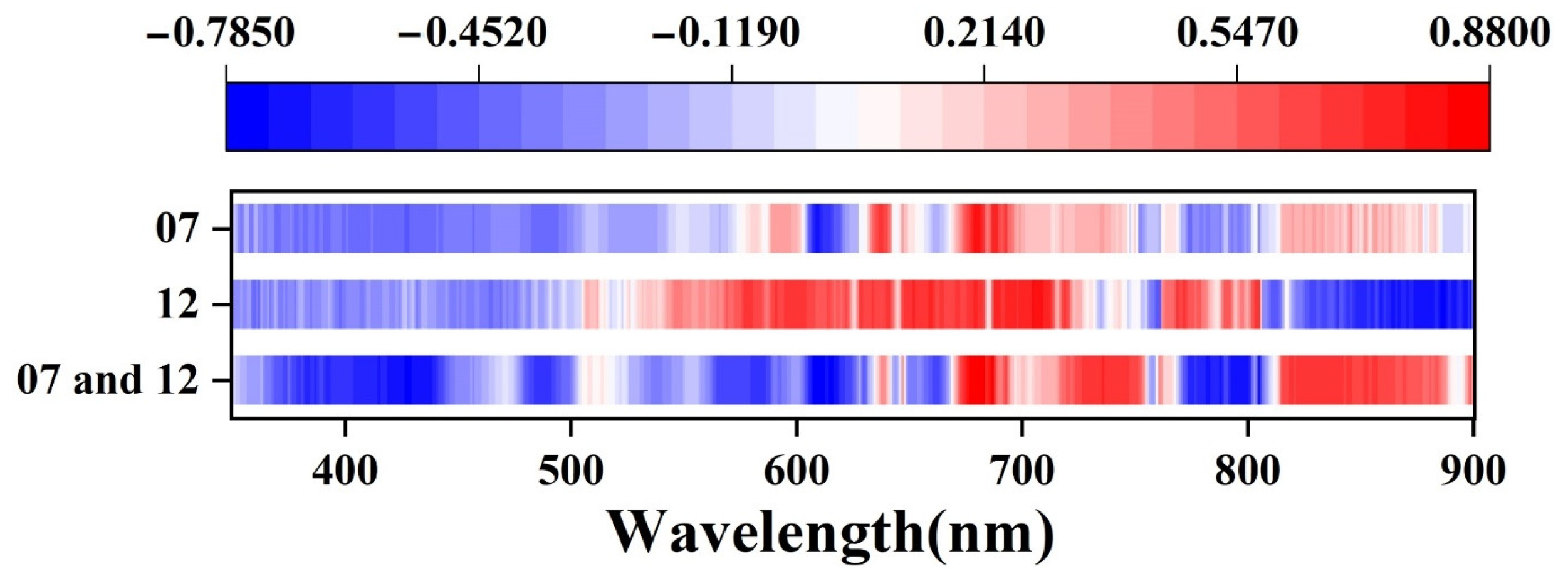
After first-derivate processing, the correlation of the data was significantly improved, and compared in Figure 10. It shows the common characteristics of these two datasets at about 640 nm and 680 nm. In July, the correlation coefficient reached −0.69 at 609 nm and the positive correlation reached 0.78 at 680 nm. The December data reached −0.73 at 886 nm and 0.78 at 706 nm. After the combination of the two datasets of July and December, the correlation coefficients reached −0.78 at 610 nm and 0.88 at 680 nm.

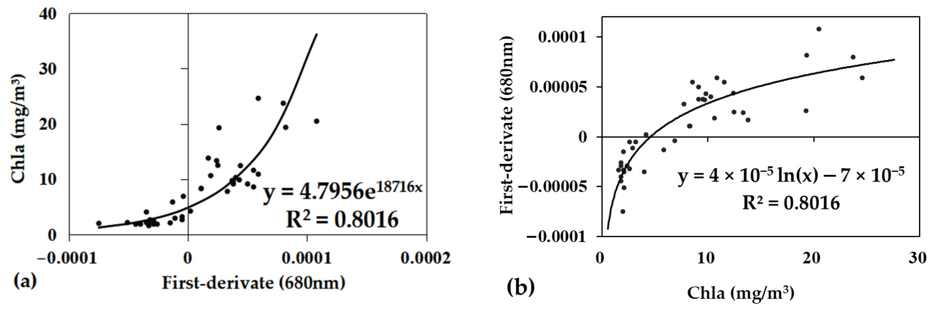
In Figure 11, the scatterplot is better fitted by an exponential function with R² above 0.8. It was verified that the trends of the two data series were the same. When modeling individually, R² in July was better than in December. When the derivate value tends to be infinitesimal, the concentration of Chla is infinitely close to 0 mg/m³, but not less than 0, which is consistent with the real situation.

The results show that the response of the first-derivate is more sensitive at a low concentration, but not at a higher concentration. When transposing the independent variable and dependent variable, the relationship will show more clearly (Figure 11b). For example, in the Chla concentration of less than 5 mg/m³, the derivate values have a sharper change, which means that low concentration has larger influence on the original reflectance near 680 nm. Zhang et al. [40] obtained a Chla concentration retrieval model for Taihu Lake using different methods, in which the regression curve of the reflectance is consistent with the trend of the reciprocal model in this study. In this model, the Chla concentration represents the x-axis and the reflection peak position represents the y-axis. This supports the conclusion in this study that the first-derivate value is more sensitive to a low concentration of Chla.

For other bands with high correlation, such as 745 nm and 805 nm, the overall R² is above 0.6, but the scatter distribution at 745 nm is slightly chaotic. Although the overall R² at 805 nm is a bit higher, the inconsistency between the datasets remains because the data correlation of the two seasons is opposite. Therefore, if we want to find a band with a better fitting result, we should consider whether the correlation coefficient of each dataset is in the same sign.

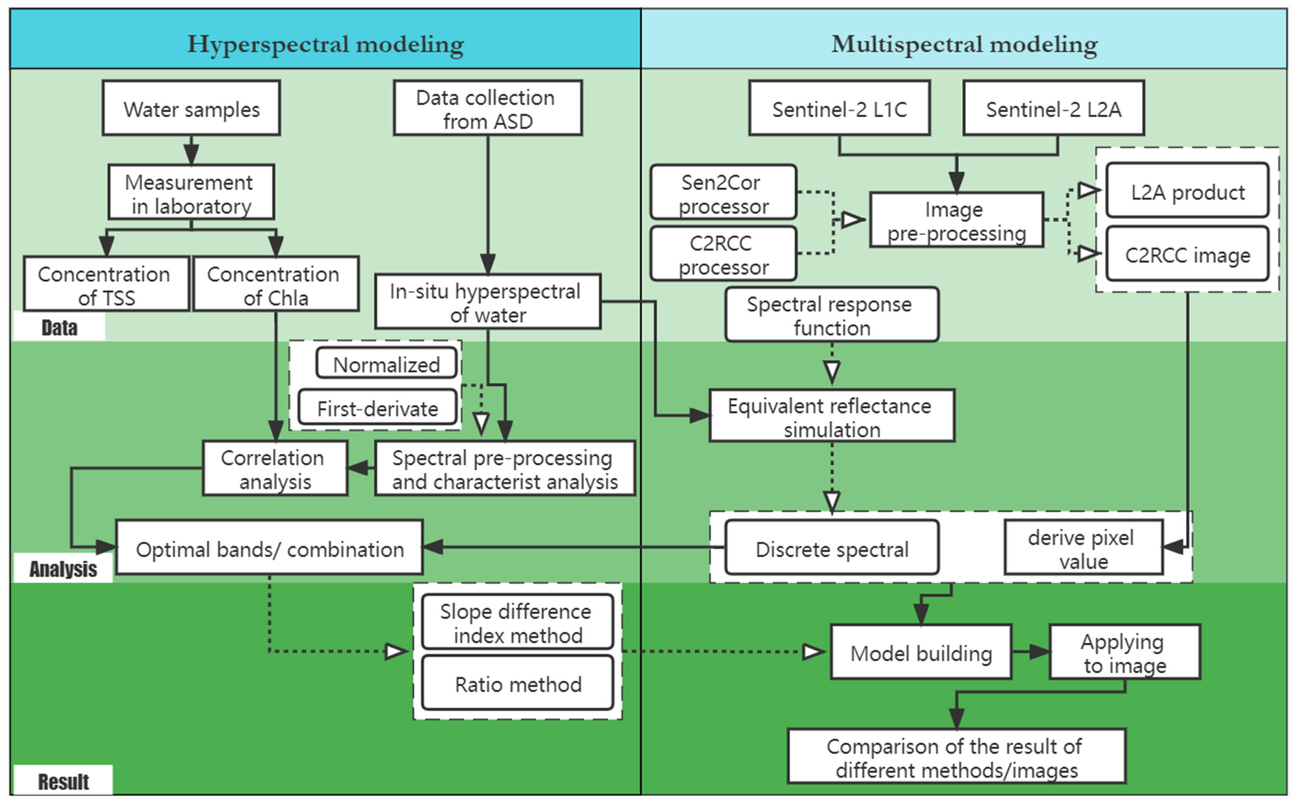
3.4. Discrete Spectral Model Based on Sentinel-2 Images

The existing satellites commonly used for water quality retrieval usually carry multispectral sensors, which have great differences from ground spectrum instruments in wavelength range, spectral resolution, and signal-to-noise ratio, meaning that optimal first-derivate modeling is difficult to apply for multispectral remote sensing images [42]. To solve this problem, the in-situ spectrum should be resampled to simulate the equivalent reflectance of sensors on the satellites [39].

This study takes Sentinel-2 as an example to explore the model of Chla based on the discrete spectrum through satellite and ground synchronous observation. The Sentinel-2 satellite is superior to many other satellites due to its high spatial resolution and data availability. It has relatively complete bands used in water quality retrieval, as shown in

Table 2. Band information for Sentinel-2A images.

Bands	Central Wavelength (nm)	Resolution (m)	Bands	Central Wavelength (nm)	Resolution (m)
B1	443	60	B8	842	10
B2	490	10	B8a	865	20
B3	560	10	B9	945	60
B4	665	10	B10	1375	60
B5	705	20	B11	1610	20
B6	740	20	B12	2190	20
B7	783	20	B8	842	10

. Previous results have confirmed its accuracy in ocean color retrieval. Yadav [46] compared the retrieval results of Chla from Landsat-8 and Sentinel-2A in Lake Pipa (fresh water) and the coastal waters of Walvis Bay (seawater), and found that the accuracy of Sentinel-2A was greater than Landsat-8. In addition, most of the existing studies on water Chla rely on direct images [23,46,47,48].

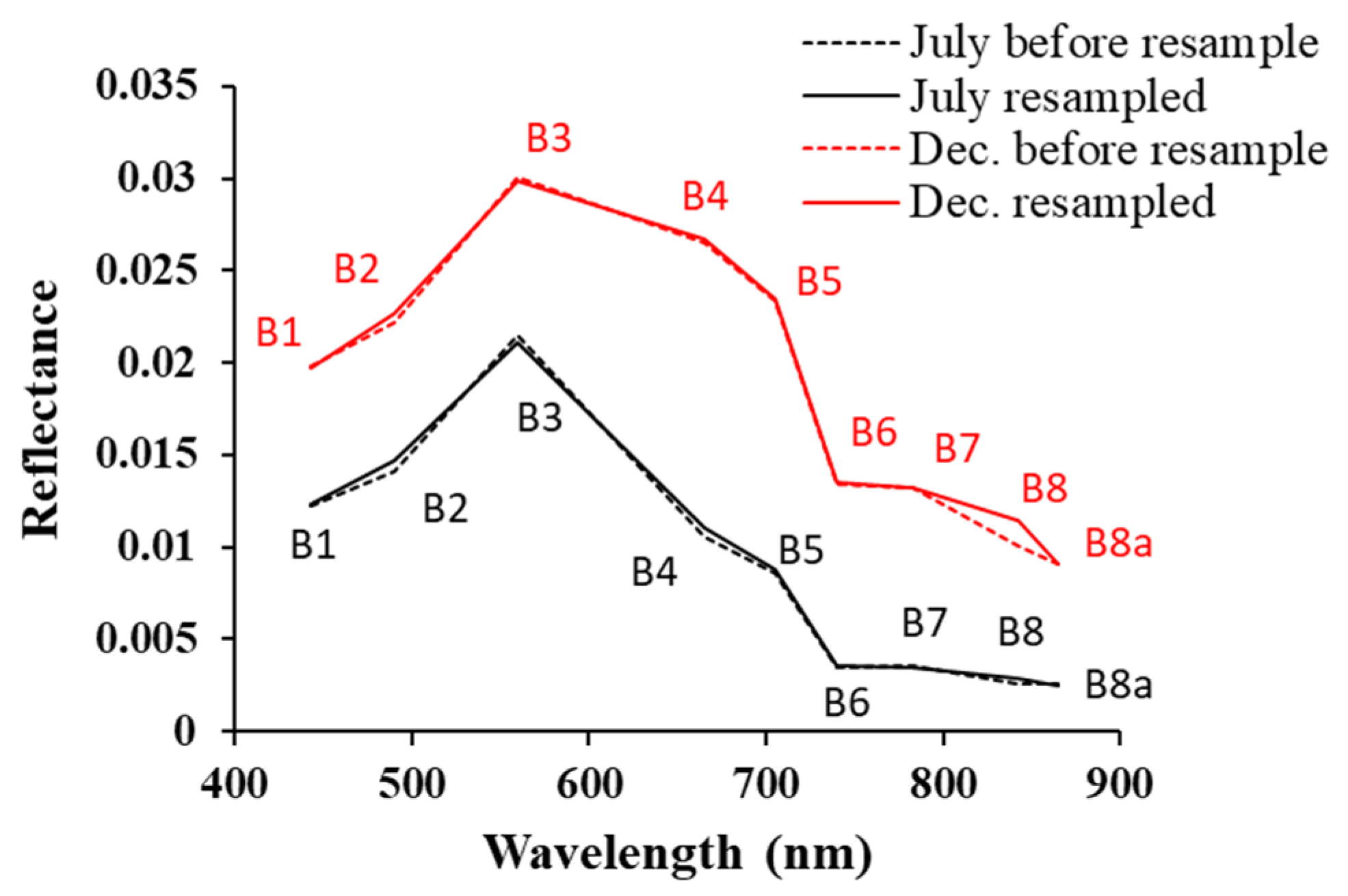
Based on the Sentinel-2 spectral response function obtained from the ESA (https://scihub.copernicus.eu/, accessed on 12 January 2021), spectral resampling was performed in ENVI 5.3 [49] to obtain the discrete bands and reflectance from in-situ spectrum corresponding to the sensor on the satellite. By comparison, it can be found that there is a slight difference between these two spectrums.

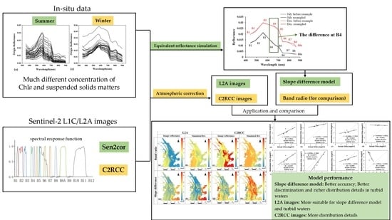
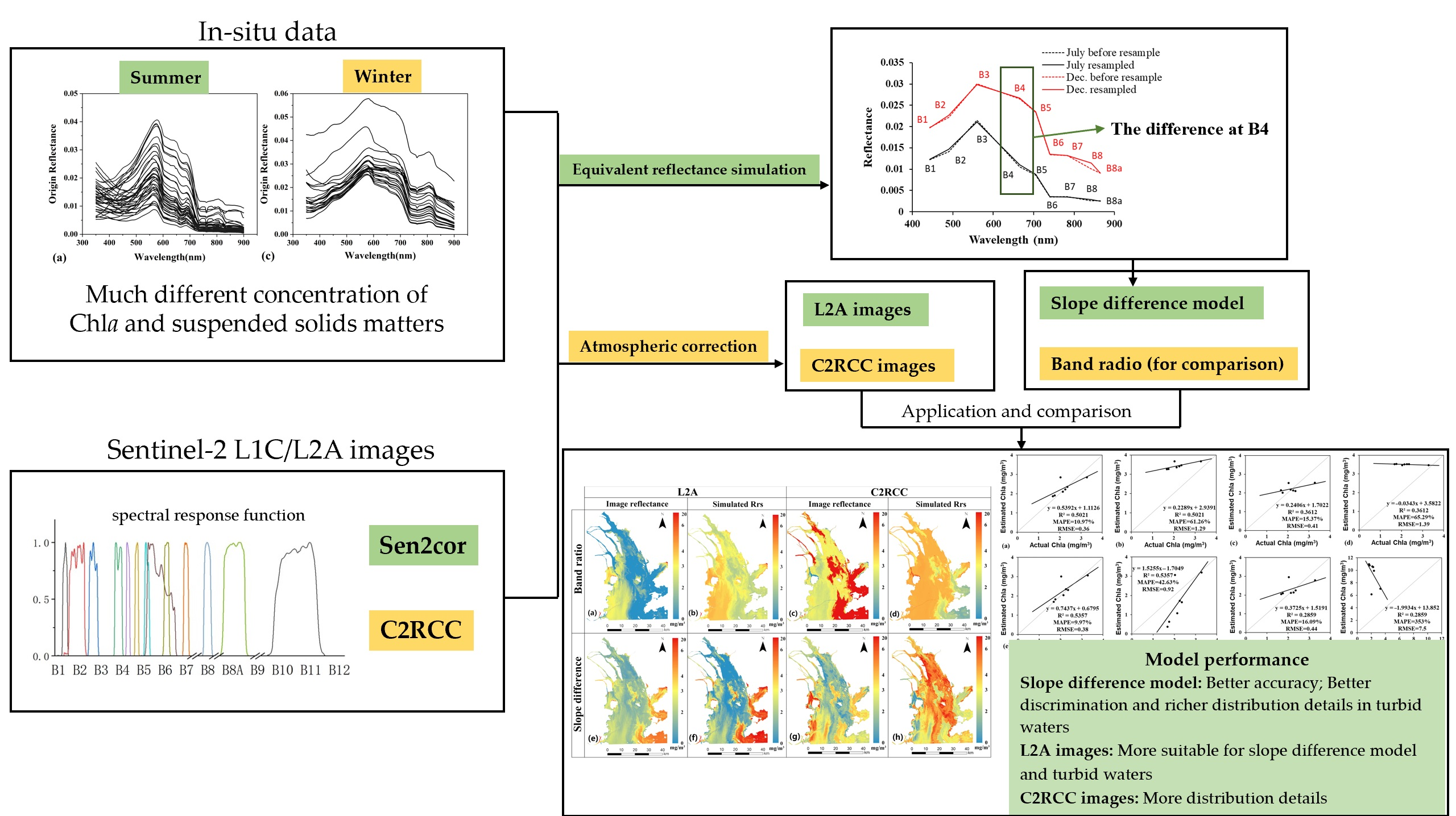
The reflectance data samples in July and December before and after resampling (by Formula (4)) are shown in the Figure 12, indicating that the reflectance and slope of each band before and after resampling have certain discrepancies. This is more obvious in B2, B3, B4, B8, which are very critical for the Chla retrieval.

3.4.1. Slope Difference Index Model

The July data is key part for whole data modeling. The normalized R_rs (705)/R_rs (665) (Figure 8c) ratio method is the same as Sentinel-2 B5/B4. The fitting result of the July data is higher. The two datasets of July and December both showed an increasing trend, but they are not exactly consistent with each other.

In Figure 12, it can be seen that in the discrete spectrum, the datasets of July and December have different fluctuation features, especially at the inflection point of B4, with different concave–convex states. The data in July were concave, but the data in December were convex. referring to the decision function established by Chen et al. [50]. In that study, the difference of the two slopes between B2, B3, and B4 of the GF-1 satellite was taken as the discriminant standard, with less than zero corresponding with convex, indicating a water body, while greater than zero corresponds with concave, indicating underwater vegetation. That discriminant results are similar to the data used in this study. Intuitively, Chla concentration is high in July and B4 of Sentinel-2 is concave, similar to underwater vegetation. In December, Chla concentration is low, suspended solids concentration is high, and B4 is convex. On this basis, a modeling method is proposed in this paper. See Section 2.3.4 for details.

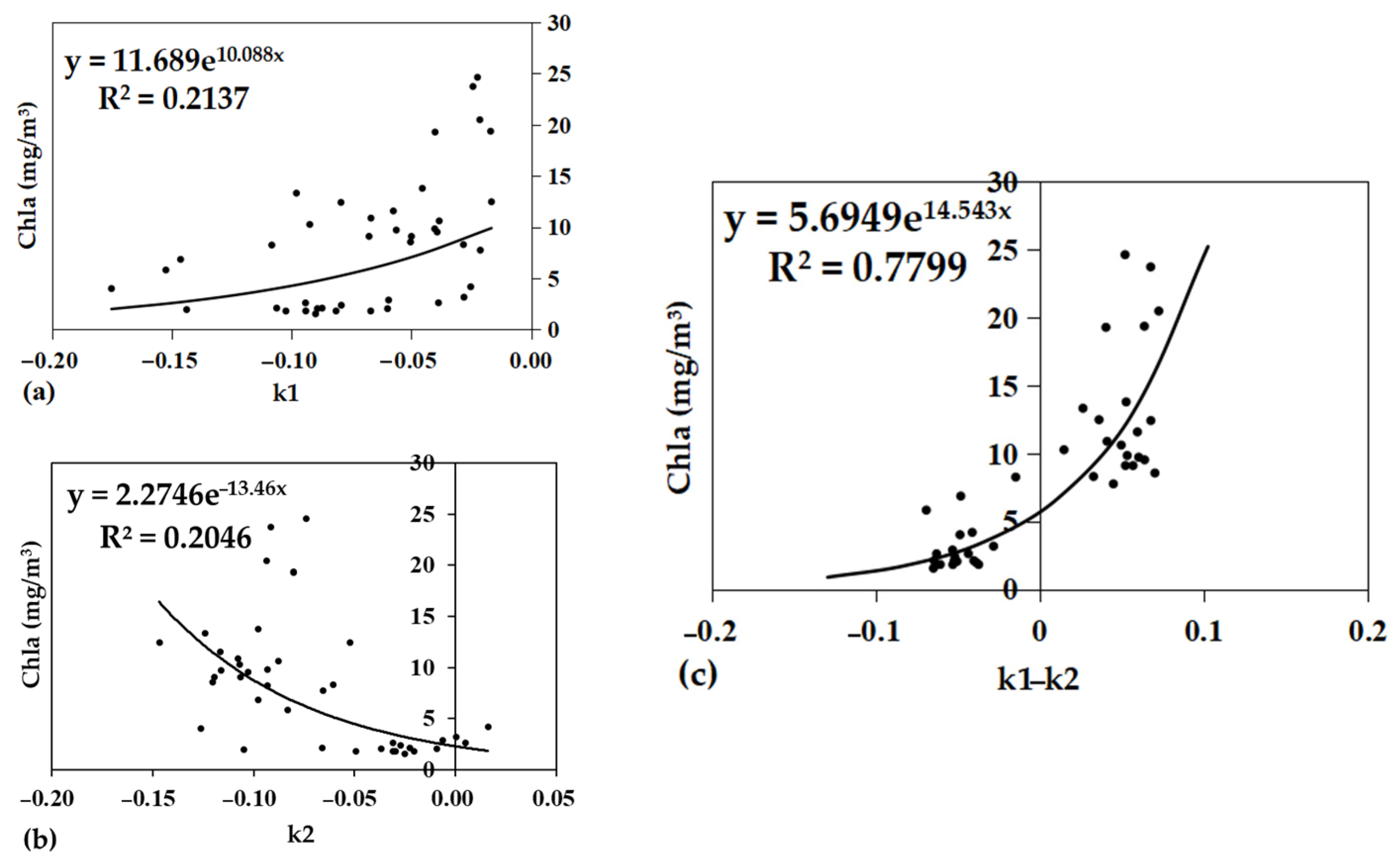
The exponential function was used for modeling based on Formula (5) with an R² value of about 0.78 (Figure 13), which is only about 0.03 lower than the R² of the optimal first-derivate model at 680 nm. In terms of band selection, the best band determined by the first-derivate model is around 680 nm of the hyperspectral spectrum, which further demonstrates the importance of this band in Chla retrieval. In the modeling of Chla, the difficulty is mainly due to the uncertain influence of suspended solids [37]. This method can obtain the integrated model of two datasets by decreasing the influence of suspended solids. The method focused on the shape of the curve instead of the absolute value of the reflectance. If applied to satellite images, the error caused by the higher reflectance of the image could be reduced.

3.4.2. Derivate Method of Discrete Spectral

In the hyperspectral model, first-derivate pre-processing of the spectrum excavates the hidden information in the continuous spectrum and establishes the retrieval model of Chla by calculating the change rate in the reflectance between adjacent bands. The model performed better than other models, but due to the limitation of spectral resolution, it cannot be directly applied to remote sensing images. This study attempts to use the discrete spectral derivate method in Chla retrieval modeling.

It should be particularly noted that the calculation of the first-derivate in ENVI 5.3 uses the default distance of 2 nm, which is only appropriate for the in-situ hyperspectral data. However, the band width in the resampled discrete spectrum is very large. In the case of a small number of bands, manual calculation can be used. Furthermore, the wavelengths before and after the middle wavelength are involved in calculation; thus, B1 (443 nm) and B8a (865 nm) are not included in the modeling.

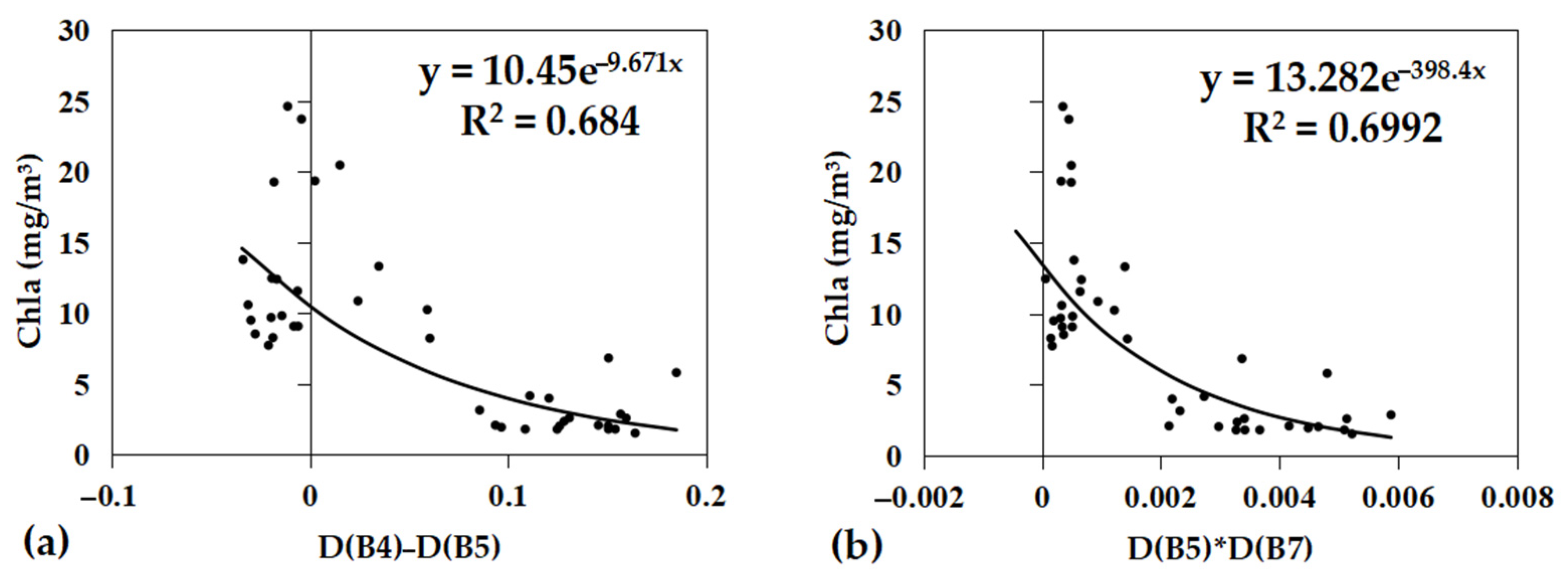
After derivate processing by the empirical algorithm, the arithmetic of band addition, subtraction, multiplication, and division was carried out. Several empirical models that can integrate the July and December data were obtained (Figure 14). By comparison, two appropriate models were obtained. The R² of the model with derivate value B4-B5 as independent variable was greater than 0.68, and the R² of B5*B7 was greater than 0.69.

3.5. Model Summary and Validation

This study used the original R_rs, normalized R_rs, and first-derivate R_rs as independent variables to set up single band models, ratio methods, and slope difference methods, aiming to build an integrated model for Chla retrieval. The evaluation of the precision of the integrated model were conducted.

It was proven that all the models are statistically significant. The R², RMSE, MAPE, MAE, and other metrics obtained for each model are shown in

Table 3. Model summary and corresponding accuracy assessment.

Data	Pre-Processing	Time	Method	Bands	Model	R2	RMSE	MAPE	MAE
Hyperspectral data from in-situ investigation	Normalization	July	Single band	673	y = 0.462x2 − 0.8083x + 0.4323	0.61	7.08	0.31	4.88
			Ratio	705/665	y = 53.531x − 31.291	0.49	4.71	0.30	4.08
		December	Single band	489	y = 18.069x2 − 43.719x + 28.307	0.78	0.46	0.19	0.40
	First-derivate	Both	Single band	680	y = 4.7956e18.716x	0.80	3.21	0.26	2.48
Discrete spectral (simulated reflectance)	Slope	Both	Slope difference	560~665~705	y = 5.6949e14.543x	0.78	5.18	0.35	3.26
	First-derivate		Subtraction	665–705	y = 10.45e−9.671x	0.68	6.99	0.47	4.26
			Multiplication	705 × 783	y = 13.282e−398.4x	0.70	6.50	0.55	4.20

. Except for the ratio method model for July, R² is greater than 0.6 for all models. However, compared with the single-band model, the ratio method model has higher accuracy, indicating that this linear model has higher stability than the unary quadratic model and is thus more suitable for the model in July. It also shows that during model selection, R² cannot be the only consideration, but it should be combined with the fitting degree between scattered points and predicted curves and the accuracy of each verification index to make a comprehensive judgment.

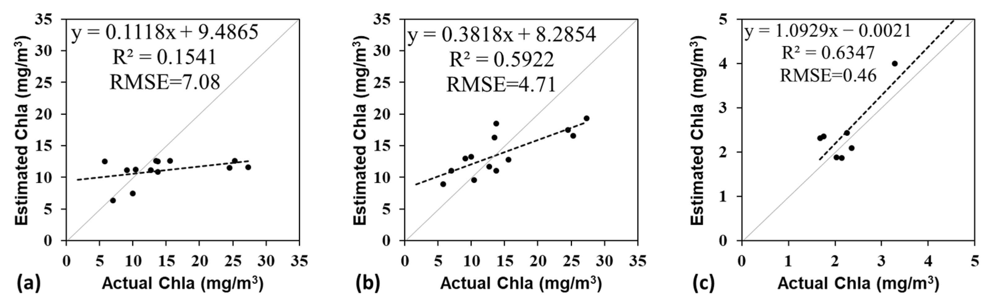
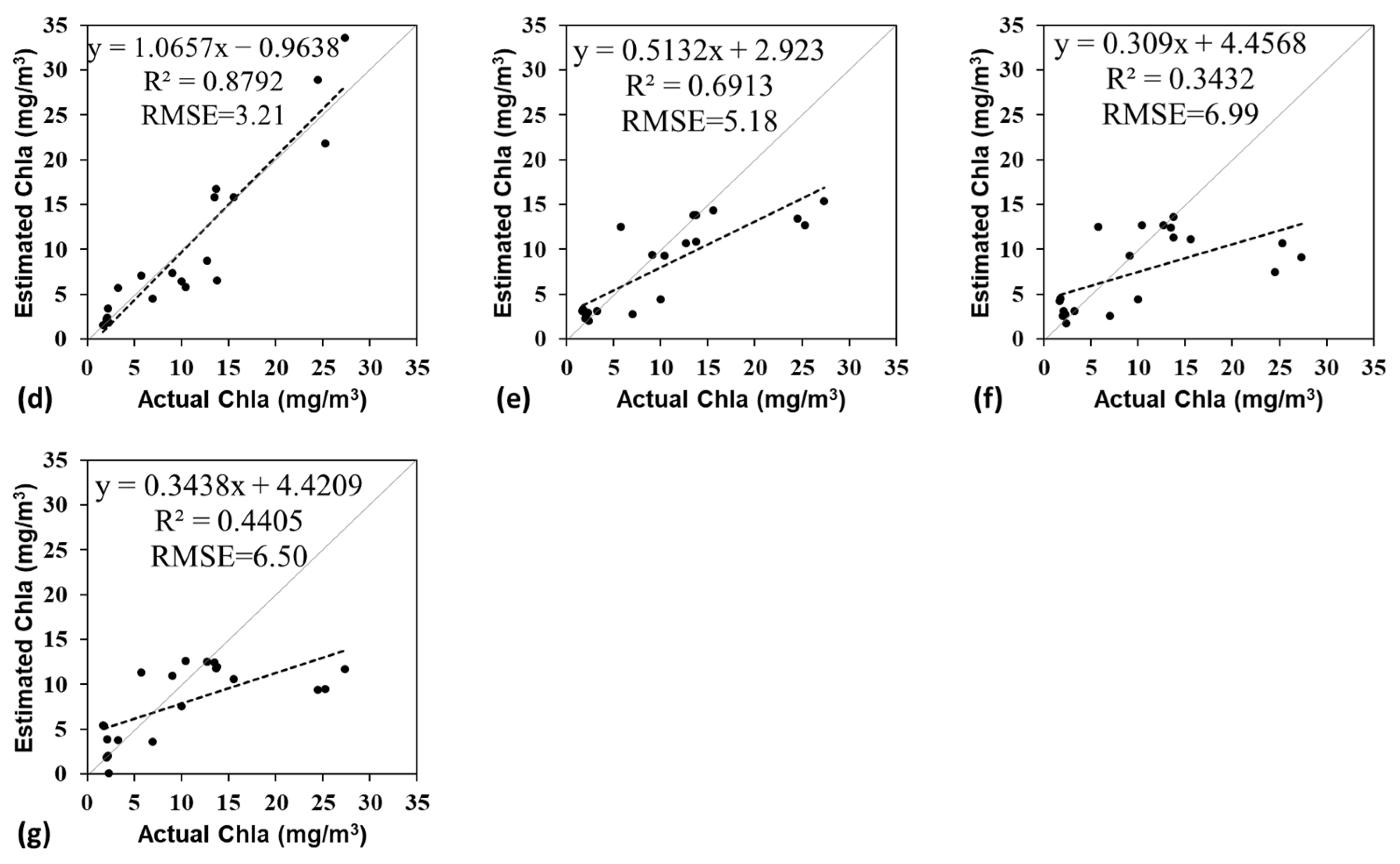
Based on the actual measured data of Chla and the estimated value of each model, the scatter plots (Figure 15) were drawn with a 1:1 line as the benchmark. The accuracy and error relationship of the models were analyzed.

It can be seen from the scatter plots between the measured and estimated values of the seven models that when Chla concentration exceeds 20 mg/m³, while the hyperspectral first-derivate 680 nm model performs better, the high concentration data are dramatically underestimated by the models. In addition, in the integrated model of these two datasets, along with the larger error of the results for the high concentration data in July, the December data also contributed a higher MAPE, even greater than the July data. This is due to the low concentration of the data in December. Although it is not far from the 1:1 line, the difference between the predicted value with maximum error and the measured data is nearly two times the measured value, especially when the concentration is less than 2 mg/m³. This error is clearly presented in the scatter plots of the separate model validation in December. In general, when the concentration of Chla is lower than 2 mg/m³ and higher than 20 mg/m³, the accuracy is low, while the errors in other concentration ranges are random.

3.6. Applicability of the Model to the Satellite Images

In order to verify the applicability of the slope difference index method, synchronous satellite images were selected for practical application. However, due to the high cloud coverage and insufficient availability of images, the Sentinel-2 L2A image product acquired on 30 December 2020, which is closest to the date of in-situ data collection, was finally selected for case study. In addition, we also tried to use the L1A product with a C2RCC processor [51] as a comparison to test the performance of the retrieval model. 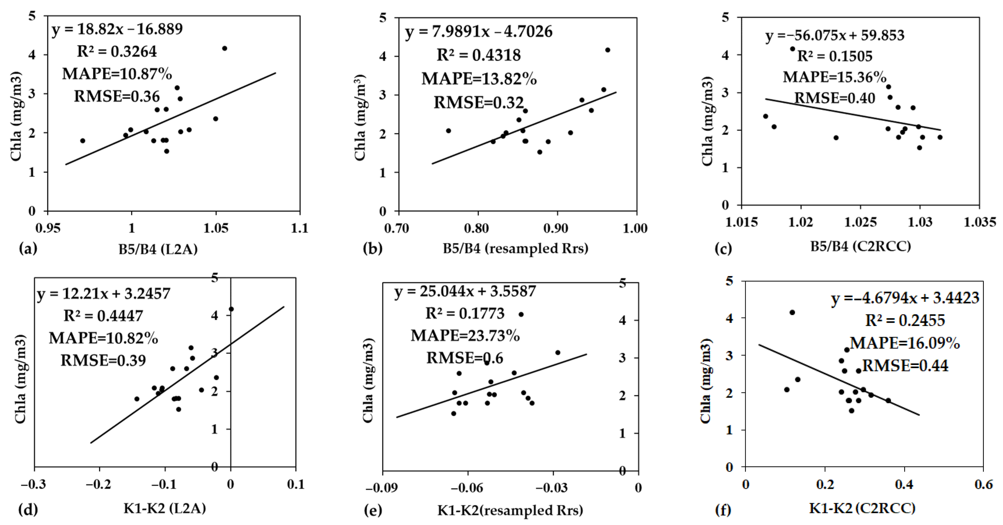Based on the simulated R_rs data from in-situ data and the reflectance derived from L2A image, the slope difference index method in this study was applied and compared with the ratio method.

To verify the model results, two-thirds of the data of December were used to retrieve Chla by the slope difference method and ratio models using the reflectance data derived from the L2A image. It can be seen that R² is quite low, and Figure 16 show that the slope difference has better accuracy for the Sentinel-2 L2A image data.

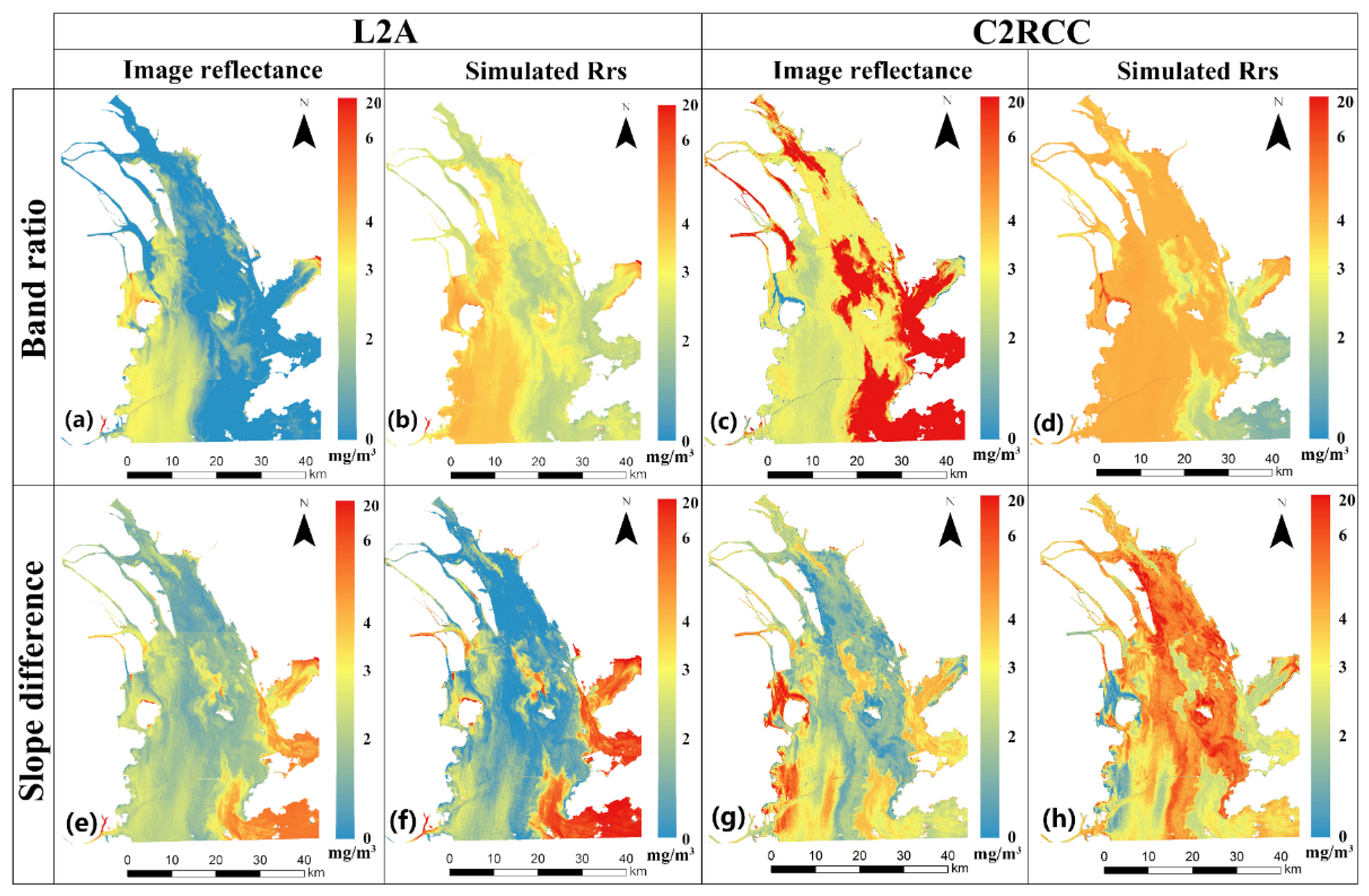
When applied to the images, it shows that the distribution of Chla concentration obtained by the ratio method was very similar to that of suspended matter, mainly distributed in the west to the middle of the PRE. The concentration was higher near Qi’ao Island and in the Shenzhen Bay. The distribution retrieved by the slope difference method was more reasonable. as Chla has better discrimination and richer distribution details in areas with different concentrations of suspended matter. The concentration was higher in the middle of PRE, Shenzhen Bay, and the coastal area of Hong Kong, China. This indicates that the proposed slope difference method can eliminate the influence of suspended matter on Chla retrieval and obtain a more realistic distribution of Chla. Figure 17b,f, shows the result of directly applying simulated R_rs to the L2A image. The distribution is basically similar to the former, but slightly overestimated.

When C2RCC products were used, the Chla distribution obtained from the ratio method is similar to that obtained from the Sentinel-2 L2A image. Both of them show a large area with the same color. However, the model and retrieval results obtained from the C2RCC image are contrary to the previous results (Figure 17a,c). When the slope difference method was used, the results of the two products were quite similar. The distribution gradation and the details of C2RCC are clearer.

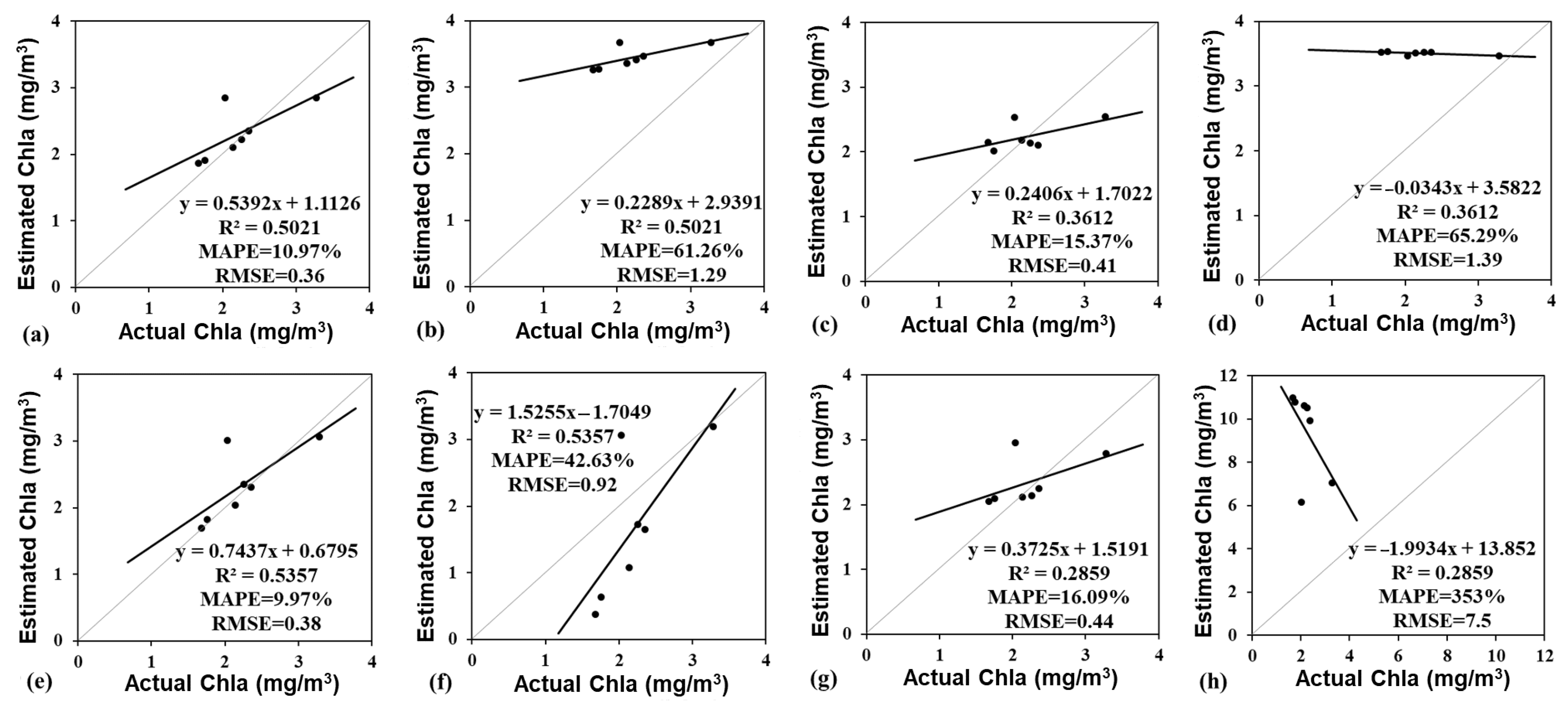
The verification results show that the accuracy of the slope difference method is slightly better than the band ratio method. When the simulated R_rs model is directly applied to the image, such as in Figure 18b,f, the results of the slope difference method (f) is more reasonable and closer to the 1:1 line. This shows that the slope difference method is less affected by the absolute value of the image and is more stable in applications. Verification with C2RCC images shows less accuracy than with L2A images. It can be seen from Figure 18c,g that the slope of Figure 18g (using the slope difference method) is closer to the 1:1 line. However, the accuracy of retrieval results obtained by the simulated R_rs was quite unsatisfactory (Figure 18d,h). This may be due to the difference between the C2RCC image spectral curve and the in-situ spectral curve. In general, L2A products may be more suitable as input image data for Chla retrieval in this study.

4. Discussion

Table 4. Comparison of Chla retrieval results from different places in the world.

Data Used First	Area	Image Source	Method	Bands Involved	Model Validation (RMSE) and Chla Range (mg/m3)	Validation of Image Retrieval Result
In-situ hyperspectral	Bangpakong River estuary (Thailand) [25]	Landsat-5	Empirical model	435, 488, 692	1.13 (0.13~7.25) Figure 16e	1.6 (0.13~7.25) Figure 18f
	Lake Huron (USA) [31]	Sentinel2-L2A	Red–NIR Ratio Multiple regression	705, 665 443, 490, 560, 665, 705, 740, 783	9.972 (1.62~51.68) Figure 15b and Figure 16b 3.127 (1.62~51.68) Figure 15e and Figure 16e	Did not show the validation, only discusses that it is similar to the real distribution
	The Bohai Sea (China) [52]	MODIS	OC4 OC3Mv6 Empirical model	443, 490, 510, 555 443, 490, 555 443, 412, 555, 490	2.36 (0~13) Figure 16e	No specific figure was given, but compared with MODIS standard Chla product, it was found that the retrieval error is large, ranging from 3~5 mg/m3
	Mundaú-Manguaba Estuarine-Lagoon System(Brazil) [53]	MODIS MERIS Sentinel-MSI/OLCI	Blue–Green Ratio NIR–Red Ratio Three-Band Four-Band	645, 555 681, 709, 665 681, 709, 674 674, 709, 681,665	14.55 (5.99~117.54) 10.44 (0.97~117.54) 5.02 (average 27.6) 7.69 (average 27.6)	Discussed the performance of different algorithms before and after classification; no images application.
Spectral from images directly	Lake Erie (USA) [4]	Sentinel2-L1C/L2A	MCI model and processor from SNAP	665, 705, 740	9.6 (0.13~88) Figure 16a,d	Compared the modeling results, not applied to images
	Some inland lakes (Brazil) [54]	Sentinel2-L1C/ C2RCC	C2RCC-C2X processor and its product from SNAP	Unclear, using the C2RCC NN model, possibly all bands	Did not build models by themselves, use the retrieval result calculated by C2RCC processor of SNAP	For different water: 1.84 (5~8) Figure 18e,g 2.26 (0~20) 2.91 (0~20)
	Three subalpine lakes and a turbid lake (Italy) [55]	Sentinel2- L1C/L2A	C2RCC MASI OC3	No details for C2RCC and MASI; 443, 490 for OC3	Compared the agreement (R2) between different algorithms	For different lakes: Subalpine (0~6); Turbid (1~25): C2RCC: 0.57; 3.2 MASI: 0.6; 2.6 OC3: 1.39; 4.1

summarizes the general results and validation from several representative Chla retrieval studies in different research areas. These include study results which used first in-situ hyperspectral data to model an then applied it to images, or directly used the reflectance of images for modeling and retrieval. They are similar to this study regarding the data, method, and validation. The images involved are mainly the Sentinel-2 images used in this study, as well as typical Landsat-5 and MODIS images. ESA provides Sentinel-2 images processed by two atmospheric correction algorithms, namely sen2cor and C2RCC. We compared the retrieval results obtained by these two algorithms. For example, Sentinel-2 L2A product used sen2cor, while the other algorithm is C2RCC. The Case 2 Regional Coast Color (C2RCC) atmospheric correction is a full spectrum version using a set of neural networks that are trained on simulated top-of-atmosphere reflectance. It was used to generate the Case 2 water products in Sentinel 3 OLCI standard ESA products, which are suitable for Sentinel-2 Multiple Spectral Image (MSI) as well. It can be operated in the free SNAP software developed by the ESA and can generate products related to Chla.

Suwisa Mahasandana et al. [25] used the in-situ hyperspectral data to build an empirical model and applied it to Landsat-5 images. The validation result is similar to Figure 18f in this study, which shows better performance, supporting that the method in this study has certain feasibility. Chen et al. [31] compared the model accuracy of the ratio method and multiple regression, and the latter was applied to Sentinel-2 L2A images using a neural network model. The validation was not given, but the author discussed that the Chla distribution was approximately the same as the real situation, meaning that the L2A product is still effective in Chla retrieval. Cui et al. [52] classified the Bohai Sea with 23 classes, using different retrieval methods for different water optical classes, and obtained accuracy better than that without classification. Finally, this method was applied to MODIS images without validation details given. The authors compared the retrieval results with the MODIS standard products and showed that the retrieval results of coastal water differed greatly, with the error ranging from 3~5 mg/m³. In the concentration range of 0~13 mg/m³, the error is obviously large, which also shows that the retrieval of coastal water is still challenging. Lins et al. [53] compared the bands-ratio, three-bands, and four-bands methods for the Mundaú-Maguaba Estuarine-Lagoon System to evaluate their performance before and after the spectra classification based on k-means clustering classification. This study evaluated the possibility of applying those algorithms to common satellite images.

Pirasteh et al. [4] used the MCI algorithm of Sentinel-2 at SNAP and the image pixel value obtained by MCI was used for modeling. By comparison, the accuracy of Figure 16a,d in this paper is greater. Sentinel-2 images with C2RCC atmospheric correction were used to compare the retrieval results in different inland waters of Brazil [54]. This study reported that C2RCC was suitable for atmospheric correction of coastal water and is better than sen2cor, especially when C2RCC-C2X was well-performed for turbidity water. The validation result is similar to Figure 18e,g in this study, but the accuracy of this paper shows that L2A images are more suitable for chlorophyll retrieval for turbid water. Niroumand-Jadidi et al. used the state-of-the-art methods of C2RCC, MASI, and OC3 to estimate the Chla using Sentinel-2 images directly. They compared the ability of those methods on lakes with different turbidity and stated the strengths and weaknesses of those methods to readers [55].

Today, it is still a challenging task to improve the accuracy of Chla retrieval based on remote sensing techniques. There are still many issues for improvement in turbid water areas, for example, whether to use atmospheric correction (sen2cor or C2RCC), or just directly use in-situ R_rs for modeling. Therefore, combining in-situ hyperspectral R_rs data with image reflectance, improving the accuracy of atmospheric correction, and choosing which model to use and whether to carry out optical classification of water bodies are all problems worth discussing in future studies.

5. Conclusions

In this study, we used 61 groups of in-situ hyperspectral data and corresponding Chla concentrations collected in July and December 2020 in the Pearl River Estuary to build a Chla retrieval model that takes the two different seasons and the turbidity of water into consideration. The ultimate aim of this study was to develop an integrated model for Chlorophyll-a retrieval based on satellite images. This improvement was necessitated by the seasonal variations in Chla concentration. Many existing studies have reported that the models show differences in representative bands and model performance. Due to the regional specificity of many models, high accuracy can be validated in one water area, but usually not in another water area. Spectral curves vary in different waters and different seasons, but changes generally fluctuate near representative bands with band width of 1~10 nm. Some researchers have also tried to discuss the seasonal data separately. However, for seasons or months without in-situ hyperspectral data, it is not possible develop appropriate models for such periods; the retrieval accuracy cannot be guaranteed either. A more universal and stable model is required to perform well in different conditions.

Thus, the ultimate aim of this study was to develop an integrated model for Chlorophyll-a retrieval based on satellite images. The results show that the hyperspectral model’s R² is above 0.8 and the MAPE is 26.03%. Among the discrete spectral models, the slope difference model is the best, with R² of about 0.78 and MAPE of 35.21%. When applied to images, it is proven that the slope difference method can be used in practice, eliminating the influence of suspended matters to a certain extent. Although the reflectance in the images is much higher than that measured on the ground, its shape and slope are similar to the ground data. The slope difference index method proposed in this study can reduce this error, which focuses on the slope of the reflectivity curve instead of the specific reflectivity value. This study provides a feasible proposal for Chla retrieval in estuarine and nearshore waters.