Article

A Network Combining a Transformer and a Convolutional Neural Network for Remote Sensing Image Change Detection

1
School of Environmental and Spatial Informatics, China University of Mining and Technology, Xuzhou 221116, China
2
Land Satellite Remote Sensing Application Center, MNR, Beijing 100048, China
*
Author to whom correspondence should be addressed.
Remote Sens. 2022, 14(9), 2228; https://doi.org/10.3390/rs14092228
Submission received: 24 March 2022 / Revised: 23 April 2022 / Accepted: 28 April 2022 / Published: 6 May 2022
(This article belongs to the Special Issue Deep Reinforcement Learning in Remote Sensing Image Processing)

Abstract

:
With the development of deep learning techniques in the field of remote sensing change detection, many change detection algorithms based on convolutional neural networks (CNNs) and nonlocal self-attention (NLSA) mechanisms have been widely used and have obtained good detection accuracy. However, these methods mainly extract semantic features on images from different periods without taking into account the temporal dependence between these features. This will lead to more “pseudo-change” in complex scenes. In this paper, we propose a network architecture named UVACD for bitemporal image change detection. The network combines a CNNs extraction backbone for extracting high-level semantic information with a visual transformer. Here, visual transformer constructs change intensity tokens to complete the temporal information interaction and suppress irrelevant information weights to help extract more distinguishable change features. Our network is validated and tested on both the LEVIR-CD and WHU datasets. For the LEVIR-CD dataset, we achieve an intersection over union (IoU) of 0.8398 and an F1 score of 0.9130. For the WHU dataset, we achieve an IoU of 0.8664 and an F1 score of 0.9284. The experimental results show that the proposed method outperforms some previous state of the art change detection methods.

Graphical Abstract

1. Introduction

Change detection is a process of identifying differences by observing the states of an object or phenomenon at different times [1]. It is one of the main problems in Earth observation and has been studied extensively in recent years. With the continuous development of Earth observation technology, a large amount of remote sensing data with hyperspectral space-time resolutions are now available, bringing new requirements for change detection and promoting the development of change detection technology. The application fields of change detection are urban expansion [2], building change detection [3,4], water environment change detection [5,6], forest detection [7], debris flow and landslide detection [8].
Most traditional change detection methods can be divided into two steps: change unit analysis, and change identification [9]. Change unit analysis usually divides the image into pixel-level units, and object-level units, and then constructs useful features based on these units. Different forms of analysis units share similar feature extraction techniques, common spectral features, and spatial features. Change identification uses human-made or learned rules to compare feature representations of analysis units to determine change categories. A common and simple method is to calculate a feature difference map and then use thresholding to segment the change region [10]. The direction and magnitude of the change vector can be analyzed to determine the type of change based on change vector analysis (CVA) [11]. Alternatively, hand-designed rules are used to construct decision trees [12], and support vector machines are used [13] to identify the type of change. In addition, probabilistic graphical models, such as Markov random field and conditional random field models, can also be used for change identification [12,13]. Thus, traditional methods of change detection are designed based on handcrafted features and supervised classification algorithms with strong theoretical explanations, but the feature construction and selection process of these methods is complex and less adaptable to unknown datasets. End-to-end deep learning (DL) methods, on the other hand, have been rapidly developed by liberating the process of tedious hand-designed features.
Over the past few years, based on convolutional neural networks (CNNs), remote sensing image change detection approaches have achieved remarkable progress. Most recently developed supervised change detection (CD) methods rely on CNN-based structures to extract high-level semantic features that reveal the change of interest from each temporal image [3,14]. However, convolution kernels are not good at modeling the long-range dependencies of image contents and features because they only process a local neighborhood, either in space or time [15]. Current change detection methods, including both feature-level Siamese change detection and image-level fusion- and segmentation-based change detection approaches, are almost all built upon convolutional operations [16,17,18]. As a consequence, these methods only perform well in modeling local image content relationships but are limited in terms of capturing long-range global interactions. The long-range global interactions indicate that we integrate the image global contextual relationships to calculate each pixel value in the image, which make the generated feature maps have more robust properties. Such a deficiency may degrade the capacities of these models to deal with scenarios where global contextual information is important for localization, such as objects undergoing large-scale land use change types. It is necessary to introduce a nonlocal self-attention mechanism to capture remote global interaction information [19,20,21].
A transformer can be seen as a special self-attention mechanism [22], that performs global adaptive weighting of inputs by computing global contextual relations to automatically focus on key information locations. Transformers have achieved rich success in tasks such as speech recognition [23] and natural language modeling [24]. Recently, transformers have been employed in discriminative computer vision models and have attracted great attention [25]. This mechanism has also received considerable attention in remote sensing image processing, such as image time-series classification [26,27], hyperspectral image classification [28], and RS image captioning [29]. However, transformers have not been widely used in remote sensing change detection. ChangeFormer [30] is a hierarchical transformer in a Siamese network with a lightweight decoder, and it shows that good results can still be obtained without relying on the convolution operation. However, it is limited by the mechanism of the transformer, which makes training the model more difficult. CNN + Transformer is another effective solution. Bit-CD [31] uses a transformer decoder network to enhance the context information of Conv-Net features. It has the advantages of the efficient training performance of convolutional networks while maintaining the advantages of long-distance dependency information modeling. The video vision transformer (ViVit) [32], is a video sequence classification network built using a visual transformer. Here, we use the idea of building spatiotemporal dependencies between frames by a transformer to construct a change intensity token and propose a new end-to-end change detection architecture for CNNs and transformers with encoder–decoders to boost the performance of conventional convolution models. Our approach differs from ViVit in two ways: first, the network structure is redesigned to adapt to the semantic segmentation task, and second, CNNs are used as the feature extraction framework for feature extraction.
Both spatial and temporal information are important for change detection. The former contains object appearance information for target localization, while the latter includes the state changes of objects. Most existing change detection methods only exploit spatial information because they apply attention separately to each temporal image to enhance its features or simply use attention to reweight the fused bitemporal feature maps in the channel or spatial dimension [21,33,34,35,36]. For example, a previous study [37] extracted multi-level features from a Siamese network for dual-temporal images and used feature differences in algebraic operations to detect used changes. Another study [38] extracted the most representative features at different semantic levels by cascading bitemporal features at different scales, and then performed channel attention on these features. Ref. [20] makes the network focus on useful information on bitemporal images by adding attention mechanisms to the Siamese networks separately.
Although successful, these methods mainly focus on extracting semantic features on images at different time periods, but do not consider the temporal dependence between these features, which will lead to more pseudo-change in complex scenes. In this work, considering its superior capacity for modeling global dependencies, we use a transformer to integrate spatial and temporal information for change detection, generating discriminative spatiotemporal features for feature fusion. Considering the superior capability of transformers in terms of modeling global dependencies, we use a transformer to integrate spatial and temporal information for change detection and generate discriminative spatiotemporal features for feature fusion. More specifically, we propose a new spatiotemporal module based on visual transformer for change information fusion. The new architecture contains three key components: an encoder, a fusion module, and a variance information extraction module. The encoder receives the original image in two time periods and generates independent feature maps. This fusion module uses the visual transformer structure to enhance independent feature maps and achieves the fusion of spatiotemporal information. The differential information extraction module is based on 3D convolution (conv3d), which is different from general algebraic operations such as summation and difference, and can more flexibly generate change feature maps and be directly used for classification.
In summary, this work has three contributions.
1. We propose a new 3D convolutional difference information extraction module specifically for the extraction of bitemporal variation feature maps. It can easily and efficiently aggregate bitemporal features, helping us to generate difference feature maps more flexibly while helping us to focus more on the feature encoding or feature enhancement part.
2. We propose a visual transformer-based spatiotemporal feature enhancement strategy in the dual-temporal feature information fusion and processing approach. Temporal information modeling is achieved by first executing the transformer separately in the spatial dimension, and then a classification token of aggregated temporal features is constructed in the temporal dimension; in other words, this approach can be understood as a global average pooling operation involving fused temporal information. The method fully considers the long-range dependencies between feature maps and unites feature information in the temporal dimension, and the experimental results show that this is important for temporal feature enhancement.
3. For the combined CNN + Transformer approach, we construct an additional training loss for the transformer part to strengthen the influence of the transformer module on the network, and experimentally validate the feasibility of this approach, which provides a new solution for the CNN + Transformer to build a change detection network.
The rest of this paper is as follows. In the second section, the overall structure of the change detection network in this paper is proposed, in which the dual-time phase feature fusion enhancement module and the feature difference module are described in detail. In the third section, the experimental results and analysis are provided. In Section 4, we discuss some of the details and parameters of the experimental results. In Section 5, the conclusions of this paper are derived.

2. Materials and Methods

In this section, we introduce the architecture of the proposed method in detail. The overall structure of the change detection network for learning spatiotemporal features is presented in Figure 1. For clarity, we first introduce this basic change detection network with three main modules: a feature extraction backbone in Section 2.1.1, a difference information extraction module in Section 2.1.2, and a decoder for segmentation in Section 2.1.3 and Section 2.1.4. Subsequently, In Section 2.2, we add a transformer-based temporal feature enhancement module to the basic network to help build a long-range modeling approach for spatiotemporal features, considering the long-range dependence of self-attention and making the network performance more robust.

2.1. Basic Siamese Network with a Conv3d-Based Differential Module

2.1.1. Siamese Backbone

The transformer locates key location information by computing global adaptive weighting for the input, which makes the computational effort of the model positively correlated with the size of the input image. ViVit [32] divides the image into blocks of nonoverlapping size and computes block-to-block correlations, and although it greatly reduces the computational effort, it loses its ability to model the relationships between pixels with a block modeling capability. However, convolutional networks perform feature extraction by sliding windows, which are less computationally intensive than a transformer. Therefore, to compensate for the computation of block-to-block correlation analysis, we use ResNet [15] as the backbone to build a deep feature extraction framework, and to guarantee the model capacity, we use ResNet50 to achieve a better feature representation. More specifically, there are no changes in the original ResNet other than the removal of the last stage and the fully connected layers. The input of the backbone is a pair of images: a pre-period image   z 1 3 × H × W , and a post-period image z 2 3 × H × W that locate the change state information. Afterward, by passing them to the backbone, the pre- and post-period images z 1 and z 2 are mapped to feature maps f z 1 C × H s × W s and f z 2 C × H s × W s , respectively. Here, s represents the size of the block. Then, for the change detection task, we constructed the change detection network backbone of this paper by using the Siamese structure, which is shown in Figure 2 below. The depth residual convolution uses the same color to indicate that they have the same network structure and weights, which will form a Siamese backbone, and then the output of different input images passing through this Siamese backbone will become different. Thus, we use different colors to draw the output.

2.1.2. Difference Information Extraction

The difference feature maps are extracted as a simple cascade of bitemporal feature maps extracted by the Siamese backbone and then operated by the 3D convolution module [39]. Unlike traditional 2D convolution, the convolution kernel of 3D convolution adds a temporal dimension to process the sequential image input, so the input feature map needs to be stacked in the temporal dimension. The processing process is shown in Equation (1). In this module, the channel width C, height H, and weight W of the bitemporal feature maps f z 1 and f z 2 are kept constant. The receptive fields on the multiscale temporal feature maps are fused by convolving the conv3d voids with dilation rates of 1, 4, and 8, and a convolution is performed for feature aggregation. Here, to fuse the receiver fields at different scales, the 3D convolution module uses the idea of atrous spatial pyramid pooling (ASPP) [39], which we name ASPP3d. Dilation = 1 represents the normal convolution, while the outer 4 and 8 are added to aggregate the difference features at multiple scales and to increase the model capacity. In addition, we visualize the absolute value of the feature map and the difference feature map extracted using ASPP3d. Figure 3 shows that the extracted features are more robust and have less noise.
D = σ ( g ( f z 1 , f z 2 ) )
where   g :   H × W × C × 2 H × W × C represents the difference feature extraction operation and σ represents the aggregation operation of g with different dilation parameters. C is the number of channels after convolution, where C = C .

2.1.3. Classification Head

Since the size resolutions of the feature maps extracted based on the ResNet backbone are smaller than the resolution of the original image, to achieve a semantic segmentation process that guarantees the size of the original image, the difference feature maps need to be upsampled and then classified by convolution. Since a simple upsampling operation produces a tessellation lattice phenomenon, an additional convolution operation is added to the sampled difference feature map to stabilize the post-sampling performance; this is followed by a categorical convolution output change probability for two classification steps. The first channel represents the background probability value with a label value of 0, and the second channel is the change foreground probability value to be extracted with a label of 1. The structure is shown in Figure 4.

2.1.4. Construction of Extra Predictions

Although the ASPP3d difference feature extraction module proposed in this paper can simply aggregate the bitemporal feature relations, it fails to consider the multiscale resolution relations of multilevel feature maps. Therefore, in this paper, the Unet [40] structure, which consists of a symmetric encoder–decoder network with skip connections to enhance detail retention, is adopted to build an extra classification. The overall process is shown in Figure 5. Here, signal “C” represents the cascading and convolution of the difference feature maps. The red and yellow parts at the bottom of the figure represent the feature maps generated by the bitemporal images after the Siamese backbone. The light blue part is their difference feature map, and the transformer is the bitemporal feature enhancement module for disparity feature extraction, which is introduced in Section 2.2.

2.1.5. Loss Function

As the change detection process used in this paper is treated as a semantic segmentation task, we use softmax cross-entropy loss in the training phase for implementation. The loss formula is as follows:
l ( x , y ) = L = ( l 1 , , l N ) τ
l n = w n [ y n × log x n + ( 1 y n ) × log ( 1 x n ) ]
where y is the true value of a point (usually 0 or 1), x is the predicted value of a point, N is the batch size, and w is the weight given to each batch. Due to the construction of a multilevel resolution prediction task, this network has a total of two losses to be calculated. The final loss_total = sum (loss1, loss2).
The smaller the subscript of the loss is, the closer it is to the final output of the network and the smaller its resolution. In the calculation of the loss, the binary label map must be resampled to this resolution.

2.2. Bitemporal Feature Enhancement

To enhance the model so that it can handle global contextual information while specifying the temporal and spatial relationships between pixel pairs to generate differentiated spatiotemporal features, we propose a bitemporal feature fusion transformer module. It mainly consists of the following two structures: tokenization in Section 2.2.1 and the spatiotemporal transformer in Section 2.2.2, as shown in Figure 6.

2.2.1. Tokenization

Vit divides an image into a series of sequences as input, scans each element of the sequence, and learns their dependencies. Although this feature makes it essentially good at capturing global information in sequence data, it cannot implicitly learn the position information of the obtained sequence, so it needs to perform position encoding on the sequence to retain the position information (position embedding, PE). The formula can be expressed as follows. To learn the relationships between temporal feature maps, a temporal classification token is used here, as shown in the formula below:
T = S ( f z 1 , f z 2 , p ) + p o s
where   S :   H s × W s × C × 2   ( ( H s p     W s p ) + 1 ) × C × 2 is the sequence that divides the input feature map into   p size patches and encodes the original feature width C as C , and change intensity tokens used to fill the time dimension are generated in this process. p o s ( H s p     W s p + 1 ) × 2 is a position-encoding parameter that can be calculated. Note that since the height H and width W of the original image will become 1/s times since the Siamese backbone from the previous section is used, image chunking is achieved, so we set p to 1.

2.2.2. Spatiotemporal Transformer

This part of the structure contains both spatial transformer and temporal transformer parts with a similar multiheaded attention mechanism. Both parts are composed of transformer encodings of L layers, with each layer containing a multiheaded self-attention mechanism (MSA) with layer normalization (LN) and a multilayer perceptron (MLP) structure, which are denoted as follows:
y l = MSA ( LN ( T l ) ) + T l
T l + 1 = MLP ( LN ( y l ) ) + y l
The MLP structure consists of two linear layers, as well as the GELU activation function, and the dimensionality C\prime of the sequence is kept constant throughout the process. In addition, the model uses a separated multiheaded attention mechanism, utilizing different heads to compute spatial attention and temporal attention separately. Its attention is defined as follows:
Attention ( Q , K , V ) = Softmax ( Q K T d k ) V
where Q = X W q ,   K = X W k ,   V = X W v , X , Q , K , V ( N / r 2 ) × C , and the sequence length is denoted N, which is divided into two types, Ns and Nt, representing the sequence lengths in the space and time dimensions, respectively. The calculation formulas are as follows.
N s = H z s p H z s p
N t = 2
The core idea of this structure is to construct the spaces Q s , K s , V s N s × C and K t , V t n t × d representing the query, key and value information of the respective dimensions. Then, multiheaded attention is used to compute spatial features   Y s = Attention   ( Q s , K s , V s ) , and the next class token dimension is taken to compute temporal features Y t = Attention   ( Q t , K t , V t ) . Finally, the temporal and spatial features are multiplied together, and the residuals are concatenated.
Y = Y s + Y s Y t

3. Experiment

From the overall structure of the network, we named the network UVACD. This is because it refers to the form of UNet, and the change detection task is realized in the ASPP3d differential information extraction module proposed by the visual transformer. We validate UVACD on two publicly available building change detection datasets: the LEVIR-CD [36] dataset and the WHU [41] dataset. The experimental results show that the proposed UVACD network outperforms recently proposed change detection methods. In this section, we start by introducing the experimental dataset. Then, we describe the details of our implementation and present the utilized evaluation metrics. Finally, we list the comparison with some other methods.

3.1. Dataset Settings

LEVIR-CD [36] is an open dataset containing 637 ultrahigh-resolution (0.5 m-resolution) Google Earth image pairs with 1024 × 1024 pixels. Images of 20 different locations in several cities in Texas were collected from 2002 to 2018, and the image pairs ranged from 5 to 14 years. The introduction of changes due to seasonal and light variations in the dataset has helped to develop effective methods for mitigating the effects of unrelated changes on actual changes. Architecture-related changes include building growth (changes from soil/grassland/hardened ground or areas under construction/new building areas) and building decay (building areas/nonbuilding areas such as soil/grassland/hardened ground). The dataset covers various types of buildings, such as villas, high-rise apartments, small garages and large warehouses. The dataset contains a total of 31,333 individual building changes, with an average of approximately 50 building changes per image pair and an average size of approximately 987 pixels per change area. Note that most of the changes are due to building growth. The author of LEVIR-CD provided a standard training/validation/test split, which assigns 70% of the samples for training, 10% for validation, and 20% for testing. Regarding the GPU memory capacity limitation, we follow the standard split proposed by reference [31]. We cut the images into small patches of size 256 × 256 with no overlap. Therefore, we obtain 7120/1024/2048 pairs of patches for training/validation/testing.
WHU [41] is a building change detection dataset consisting of two-period aerial images, each with a resolution of 0.3 m. This dataset covers an area where a 6.3-magnitude earthquake has occurred in February 2011 that was rebuilt in the following years. This dataset consists of aerial images obtained in April 2012 that contain 12,796 buildings in 20.5 km2 (16,077 buildings in the same area in the 2016 dataset). A standard split does not exist for this dataset. Different researchers use different data splitting approaches to validate their models. For comparison, we use the splitting approach that was used in reference [21]. We crop the images into small patches of size 256 × 256 with no overlap. Note that we adopt the method of fewer training set samples, so we split them into three parts (4491/498/2700) for training/validation/testing according to the range of test set vectors given by the original dataset, where the validation set obtained represents 10% of the training set. See Table 1 and Figure 7 for more details.

3.2. Training Details

Our model is based on PyTorch and trained on one ubuntu20.04 operating system using four NVIDIA Tesla V100 GPUs; the training strategy uses distributed data parallel (DDP). During the training process, we implemented a loading data process where we normalized the image data to between 0 and 1 and transformed their distribution to a standard normal distribution. Then, data enhancement, random probability value of 0.5 data enhancement by random inversion, random resize, random cropping, Gaussian noise, and random color change were performed. We used cross-entropy loss and the AdamW optimizer with the parameters set to a weight decay of 0.01. The initial learning rate was set to 0.005, and the initial four epochs were dropped to 1 × 10⁻⁶ using linear warmup to the initial learning rate, followed by cosine annealing. The number of epochs was 200, and the batch size was 32.

3.3. Evaluation Metrics

To compare the performance of our model with the performances of other methods, we report their F1 and intersection over union (IoU) scores with regard to the change class as the primary quantitative indices. Additionally, we report the precision and recall values for the change category and the overall accuracy (OA) performance of the change detection task. The IoU and F1 values range from 0 to 1, and the higher each value is, the better the performance. The IoU and F1 scores are calculated as follows, where TP denotes true positives, FP denotes false positives, and FN denotes false negatives.
IoU = TP TP + FP + FN
F 1 = 2 precision recall precision + recall
The precision is calculated as:
precision = TP TP + FP
The recall is calculated as:
recall = TP TP + FN
The OA is calculated as:
OA = TP + TN TP + FN + TN + FP

3.4. Comparison with Other Methods

In this section, we compare the change detection performance of our UVACD approach with the performances of some existing deep learning change detection methods. The methods used for comparison are as follows:
  • FC-EF [37]: This method concatenates original bitemporal images and processes them through ConvNet to detect changes.
  • FC-Siam-D [37]: This is a feature-level difference method that extracts the multilevel features of bitemporal images from a Siamese ConvNet and uses feature differences in algebraic operations to detect changes.
  • FC-Siam-Conc [37]: This is a feature-level concatenation method that extracts the multilevel features of bitemporal images from a Siamese ConvNet, and feature concatenation in the channel dimension is used to detect changes.
  • DTCDSCN [19]: This is an attention-based, feature-level method that utilizes a dual attention module (DAM) to exploit the interdependencies between the channels and spatial positions of ConvNet features to detect changes.
  • STANet [36]: This is another attention-based, feature-level network for CD that integrates a spatial–temporal attention mechanism to detect changes.
  • IFNet [14]: This is a multiscale feature-level method that applies channel attention and spatial attention to the concatenated bitemporal features at each level of the decoder. A supervised loss is computed at each level of the decoder. We use multi-loss training strategies inspired by this technique.
  • SNUNet [38]: This is a multiscale feature-level concatenation method in which a densely connected (NestedUNet) Siamese network is used for change detection.
  • BIT [31]: This is a transformer-based, feature-level method that uses a transformer decoder network to enhance the context information of ConvNet features via semantic tokens; this is followed by feature differencing to obtain the change map.
  • ChangeFormer [30]: This is a pure transformer feature-level method that uses a transformer encoder–decoder network to obtain the change map directly.

3.4.1. Experimental Results Obtained on the WHU Dataset

In this section, we present the results of the comparison of UVACD with some other change detection algorithms on the WHU dataset. The comparison is mainly based on the work of [21], who tested many change methods with their splitting approach. Here, we also crop the image to a nonoverlapping 256 × 256 size, although we use less training data to train the network on the WHU dataset. We present the comparative results in Table 2. The table shows that UAVCD has shown excellent performance on this dataset. Our methods achieved F1, IOU, recall, and precision values of 1.8%, 1.74%, 0.57%, and 0.88%, respectively.
We also plotted some of the inference results from the test set, as shown in Figure 8. In the first three columns, we present the bitemporal images (A, B) and ground truths (GTs). The fourth column shows the change masks for UVACD. To show the test results more visually, the missing false negative (FN) parts are shown in green, the false positive parts are shown in red, and the other parts that overlap the label image are color-matched. Overall, UVACD is maintained on the contour shape of the image with fewer FPs. From the results of the first image, the change of the building is not simply an exclusive OR (XOR) relationship, but also includes a building to another building change relationship, which our algorithm can still accurately identify. However, from the third row of the image, the performance of our small target detection method is weakened.

3.4.2. Experimental Results Obtained on the LEVIR-CD Dataset

In this section, we compare UVACD with some other change detection algorithms on the LEVIR-CD dataset. The comparison is mainly based on the work of [30], who tested many change detection methods with their splitting approach. Moreover, we maintain a consistent way of dividing the data. We present the comparative results in Table 3. The table shows that UVACD has greater performance on this dataset. In comparison to the second-ranked metrics, the F1 and IOU values of our approach increase by 0.9% and 1.8%, respectively, but the recall and precision remain optimal.
Ref. [30] published their code and the results of a test image for their comparison experiment. We also validated their test images by inference, as shown in Figure 9. Here, we focus on the red boxes in A (pre-period image) and B (post-period image), which have changed with the disappearance of the building and the unlabeled change type. Our UVACD and Bit-CD method are still accurate in detecting the types of missing changes, but the methods used to compare them all fail to detect the types of irrelevant changes. As highlighted in red (false detection) and green (missed detection), our UVACD method maintains better robustness against building additions and reductions, and even suspected building additions, than the other change detection methods. Both of these quantitative and qualitative comparisons show the superiority of our proposed method for conducting change detection with bitemporal images.

4. Discussion

4.1. Effects of Transformers on the Network Structure

To verify the impact of the bitemporal feature enhancement module built on the transformer for the overall network structure in this paper, we designed the following sets of ablation experiments.
  • Base_Single: Only the ASPP3d convolution fusion module proposed in this paper is used (without extra classification).
  • Base_Muti: The Aspp3d convolution fusion module proposed in this paper is used for extra classification.
  • UVA_Single: The proposed ASPP3d convolution fusion module is combined with bitemporal feature enhancement without extra classification.
  • UVA_Muti: The proposed ASPP3d convolution fusion module is combined with bitemporal feature enhancement for extra classification.
The results of these four experiments on the WHU dataset and the LEVIR-CD dataset are presented in Table 4. The base network, with or without extra classification, does not significantly improve the following five metrics and is not optimal in terms of recall. When bitemporal feature enhancement is used, the prefix for UVA, the recall increases significantly, and the maximum increases in recall on LEVIR-CD and WHU are 2.25% and 1.16%, respectively. When we use the extra classification, the F1 and IoU metrics of Uva_Muti increase by 0.66% and 1.1% compared to those of Uva_Single on the LEVIR-CD dataset, but the metrics increase by only 0.09% and 0.67% on the WHU dataset. This shows that the addition of extra classification tasks has a facilitating effect on the construction of the bitemporal feature enhancement strategy. However, the facilitation of this strategy is much better on the LEVIR-CD dataset than on the WHU dataset, which may be because the change types on the LEVIR-CD dataset are more complex than those on the WHU dataset, and the test metrics of WHU are better than those of LEVIR-CD, which makes the ability of the visual transformer to cope with more complex change types more fully exploited.
We further plot the inference for the test sets of these four experiments on these two datasets in Figure 10. The first three lines in the figure represent the results on the WHU dataset, and the last three lines represent the results on the LEVIR dataset. In the first three columns, we present the bitemporal images A (pre-period image), B (post-period image) and GTs. The last four columns show the results of the four ablation experiments constructed in this paper. The UVA prefix indicates that we are using the transformer bitemporal feature enhancement strategy. Here, green represents FNs, red represents FPs, white represents TPs, and black represents TNs. From the image on the first line, we see that the ability of the network to detect small target changes has improved slightly with the addition of a transformer, but there are still omissions. In the six-line image that follows, building the transformer shows some similarity in error detection, as shown by the red part of the image, if there is no additional classification task. Here, we consider that without additional classification constraints, the overall performance of the network will be biased toward the performance of the convolutional neural network. Therefore, it is necessary to build additional classification constraints on the transformer here.

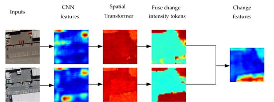
4.2. Visualization of Change Intensity Tokens

Since the Siamese backbone is used for extracting the feature maps of the pre- and post-temporal phases separately, it is important to consider these two feature maps for transformer modeling. Here, we fuse temporal information by constructing a change intensity token for each of the two feature maps, which can be computed by the transformer in the spatial dimension; then, the two calculated change intensity tokens are further computed interactively by using the transformer. To further display the feature extraction ability of the proposed transformer bitemporal feature enhancement, a gradient-weighted class activation map (G-CAM) is adopted to evaluate the proposed method. The G-CAM method displays the important areas in the image predicted by the model by generating a rough attention map from the last layer of the neural network. Red denotes higher attention values, and blue denotes lower values, as shown in Figure 11.
From the second column to the third column, we can see that the transformer has successfully located the building information on the high-level semantic feature map extracted by the CNN. However, it is redder, which indicates that it still maintains a higher weight for nonbuilding. By introducing change intensity tokens, the weight values of nonbuilding areas are obviously suppressed, resulting in a light green color. The last column of the change feature map shows that it is clearly positioned in the change area, within which the color is biased toward red.

5. Conclusions

Current deep learning-based change detection methods mainly extract semantic features on images from different time periods without considering the temporal correlation between these features. This will lead to more “pseudo-change” in complex scenes. To address this problem, we propose a network architecture for bitemporal image change detection named UVACD. The network combines a CNNs extraction backbone for extracting high-level semantic information with a visual transformer. Here, visual transformer constructs change intensity tokens to complete the temporal information interaction and suppress irrelevant information weights to help extract more distinguishable change features. The experimental results show that the proposed method is effective and outperforms some previous state of the art change detection methods. The results also show that constructing extra classification tasks for the output of the transformer can improve the performance of the network. However, our method still lacks the ability to detect changes in small targets, and there is still room for improvement. Our future work is dedicated to further modeling the ability to detect changes in small targets.

Author Contributions

Conceptualization, G.W. and B.L.; methodology, G.W.; validation, B.L. and T.Z.; writing—original draft preparation, G.W. and B.L.; writing—review and editing, G.W. and T.Z.; supervision, S.Z. All authors have read and agreed to the published version of the manuscript.

Funding

This research was funded by The National Key Research and Development Program of China, grant number 2018XXXXXXXX0N.

Data Availability Statement

Data associated with this research are available online. The LEVIR-CD dataset is available for download at https://justchenhao.github.io/LEVIR/ (accessed on 23 March 2022). The WHU dataset is available for download at https://study.rsgis.whu.edu.cn/pages/download/building_dataset.html (accessed on 23 March 2022).

Conflicts of Interest

The authors declare no conflict of interest.

References

  1. Singh, A. Review article digital change detection techniques using remotely-sensed data. Int. J. Remote Sens. 1989, 10, 989–1003. [Google Scholar] [CrossRef] [Green Version]
  2. Sandric, I.; Mihai, B.; Savulescu, I.; Suditu, B.; Chitu, Z. Change detection analysis for urban development in Bucharest-Romania, using high resolution satellite imagery. In Proceedings of the 2007 Urban Remote Sensing Joint Event, Paris, France, 11–13 April 2007; pp. 1–8. [Google Scholar]
  3. Wang, M.; Tan, K.; Jia, X.; Wang, X.; Chen, Y. A deep siamese network with hybrid convolutional feature extraction module for change detection based on multi-sensor remote sensing images. Remote Sens. 2020, 12, 205. [Google Scholar] [CrossRef] [Green Version]
  4. Li, L.; Wang, C.; Zhang, H.; Zhang, B.; Wu, F. Urban building change detection in SAR images using combined differential image and residual u-net network. Remote Sens. 2019, 11, 1091. [Google Scholar] [CrossRef] [Green Version]
  5. Clement, M.A.; Kilsby, C.; Moore, P. Multi-temporal synthetic aperture radar flood mapping using change detection. J. Flood Risk Manag. 2018, 11, 152–168. [Google Scholar] [CrossRef]
  6. Sarp, G.; Ozcelik, M. Water body extraction and change detection using time series: A case study of Lake Burdur, Turkey. J. Taibah Univ. Sci. 2017, 11, 381–391. [Google Scholar] [CrossRef] [Green Version]
  7. Housman, I.W.; Chastain, R.A.; Finco, M.V. An evaluation of forest health insect and disease survey data and satellite-based remote sensing forest change detection methods: Case studies in the United States. Remote Sens. 2018, 10, 1184. [Google Scholar] [CrossRef] [Green Version]
  8. Washaya, P.; Balz, T.; Mohamadi, B. Coherence change-detection with sentinel-1 for natural and anthropogenic disaster monitoring in urban areas. Remote Sens. 2018, 10, 1026. [Google Scholar] [CrossRef] [Green Version]
  9. Cheng, H.; Wu, H.; Zheng, J.; Qi, K.; Liu, W. A hierarchical self-attention augmented Laplacian pyramid expanding network for change detection in high-resolution remote sensing images. ISPRS J. Photogramm. Remote Sens. 2021, 182, 52–66. [Google Scholar] [CrossRef]
  10. Hao, M.; Shi, W.; Zhang, H.; Li, C. Unsupervised change detection with expectation-maximization-based level set. IEEE Geosci. Remote Sens. Lett. 2013, 11, 210–214. [Google Scholar] [CrossRef]
  11. Chen, J.; Gong, P.; He, C.; Pu, R.; Shi, P. Land-use/land-cover change detection using improved change-vector analysis. Photogramm. Eng. Remote Sens. 2003, 69, 369–379. [Google Scholar] [CrossRef] [Green Version]
  12. Gong, J.; Hu, X.; Pang, S.; Li, K. Patch matching and dense CRF-based co-refinement for building change detection from Bi-temporal aerial images. Sensors 2019, 19, 1557. [Google Scholar] [CrossRef] [Green Version]
  13. Gong, M.; Su, L.; Jia, M.; Chen, W. Fuzzy clustering with a modified MRF energy function for change detection in synthetic aperture radar images. IEEE Trans. Fuzzy Syst. 2013, 22, 98–109. [Google Scholar] [CrossRef]
  14. Zhang, C.; Yue, P.; Tapete, D.; Jiang, L.; Shangguan, B.; Huang, L.; Liu, G. A deeply supervised image fusion network for change detection in high resolution bi-temporal remote sensing images. ISPRS J. Photogramm. Remote Sens. 2020, 166, 183–200. [Google Scholar] [CrossRef]
  15. He, K.; Zhang, X.; Ren, S.; Sun, J. Deep residual learning for image recognition. In Proceedings of the IEEE Conference on Computer Vision and Pattern Recognition, Las Vegas, NY, USA, 26 June–1 July 2016; pp. 770–778. [Google Scholar]
  16. Du, B.; Ru, L.; Wu, C.; Zhang, L. Unsupervised Deep Slow Feature Analysis for Change Detection in Multi-Temporal Remote Sensing Images. IEEE Trans. Geosci. Remote Sens. 2018, 57, 9976–9992. [Google Scholar] [CrossRef] [Green Version]
  17. Mou, L.; Bruzzone, L.; Zhu, X.X. Learning Spectral-Spatial-Temporal Features via a Recurrent Convolutional Neural Network for Change Detection in Multispectral Imagery. IEEE Trans. Geosci. Remote Sens. 2018, 57, 924–935. [Google Scholar] [CrossRef] [Green Version]
  18. Zhang, H.; Gong, M.; Zhang, P.; Su, L.; Shi, J. Feature-Level Change Detection Using Deep Representation and Feature Change Analysis for Multispectral Imagery. IEEE Geosci. Remote Sens. Lett. 2016, 13, 1666–1670. [Google Scholar] [CrossRef]
  19. Liu, Y.; Pang, C.; Zhan, Z.; Zhang, X.; Yang, X. Building change detection for remote sensing images using a dual-task constrained deep siamese convolutional network model. IEEE Geosci. Remote Sens. Lett. 2020, 18, 811–815. [Google Scholar] [CrossRef]
  20. Chen, J.; Yuan, Z.; Peng, J.; Chen, L.; Huang, H.; Zhu, J.; Liu, Y.; Li, H. DASNet: Dual attentive fully convolutional siamese networks for change detection in high-resolution satellite images. IEEE J. Sel. Top. Appl. Earth Obs. Remote Sens. 2020, 14, 1194–1206. [Google Scholar] [CrossRef]
  21. Peng, X.; Zhong, R.; Li, Z.; Li, Q. Optical remote sensing image change detection based on attention mechanism and image difference. IEEE Trans. Geosci. Remote Sens. 2020, 59, 7296–7307. [Google Scholar] [CrossRef]
  22. Dosovitskiy, A.; Beyer, L.; Kolesnikov, A.; Weissenborn, D.; Zhai, X.; Unterthiner, T.; Dehghani, M.; Minderer, M.; Heigold, G.; Gelly, S. An image is worth 16x16 words: Transformers for image recognition at scale. arXiv 2020, arXiv:2010.11929. [Google Scholar]
  23. Tian, Z.; Yi, J.; Bai, Y.; Tao, J.; Zhang, S.; Wen, Z. Synchronous transformers for end-to-end speech recognition. In Proceedings of the ICASSP 2020-2020 IEEE International Conference on Acoustics, Speech and Signal Processing (ICASSP), Virtually, 4–8 May 2020; pp. 7884–7888. [Google Scholar]
  24. Devlin, J.; Chang, M.-W.; Lee, K.; Toutanova, K. Bert: Pre-training of deep bidirectional transformers for language understanding. arXiv 2018, arXiv:1810.04805. [Google Scholar]
  25. Khan, S.; Naseer, M.; Hayat, M.; Zamir, S.W.; Khan, F.S.; Shah, M. Transformers in vision: A survey. ACM Comput. Surv. (CSUR) 2021. [Google Scholar] [CrossRef]
  26. Li, Z.; Chen, G.; Zhang, T. A CNN-transformer hybrid approach for crop classification using multitemporal multisensor images. IEEE J. Sel. Top. Appl. Earth Obs. Remote Sens. 2020, 13, 847–858. [Google Scholar] [CrossRef]
  27. Yuan, Y.; Lin, L. Self-supervised pretraining of transformers for satellite image time series classification. IEEE J. Sel. Top. Appl. Earth Obs. Remote Sens. 2020, 14, 474–487. [Google Scholar] [CrossRef]
  28. He, J.; Zhao, L.; Yang, H.; Zhang, M.; Li, W. HSI-BERT: Hyperspectral image classification using the bidirectional encoder representation from transformers. IEEE Trans. Geosci. Remote Sens. 2019, 58, 165–178. [Google Scholar] [CrossRef]
  29. Shen, X.; Liu, B.; Zhou, Y.; Zhao, J. Remote sensing image caption generation via transformer and reinforcement learning. Multimed. Tools Appl. 2020, 79, 26661–26682. [Google Scholar] [CrossRef]
  30. Bandara, W.; Patel, V.M. A Transformer-Based Siamese Network for Change Detection. arXiv 2022, arXiv:2201.01293. [Google Scholar]
  31. Chen, H.; Qi, Z.; Shi, Z. Remote sensing image change detection with transformers. IEEE Trans. Geosci. Remote Sens. 2021, 60, 21546965. [Google Scholar] [CrossRef]
  32. Arnab, A.; Dehghani, M.; Heigold, G.; Sun, C.; Lučić, M.; Schmid, C. Vivit: A video vision transformer. In Proceedings of the IEEE/CVF International Conference on Computer Vision, Montreal, QC, Canada, 11–17 October 2021; pp. 6836–6846. [Google Scholar]
  33. Shi, Q.; Liu, M.; Li, S.; Liu, X.; Wang, F.; Zhang, L. A deeply supervised attention metric-based network and an open aerial image dataset for remote sensing change detection. IEEE Trans. Geosci. Remote Sens. 2021, 60, 21518766. [Google Scholar] [CrossRef]
  34. Zhang, L.; Hu, X.; Zhang, M.; Shu, Z.; Zhou, H. Object-level change detection with a dual correlation attention-guided detector. ISPRS J. Photogramm. Remote Sens. 2021, 177, 147–160. [Google Scholar] [CrossRef]
  35. Pang, S.; Zhang, A.; Hao, J.; Liu, F.; Chen, J. SCA-CDNet: A robust siamese correlation-and-attention-based change detection network for bitemporal VHR images. Int. J. Remote Sens. 2021, 1–22. [Google Scholar] [CrossRef]
  36. Chen, H.; Shi, Z. A spatial-temporal attention-based method and a new dataset for remote sensing image change detection. Remote Sens. 2020, 12, 1662. [Google Scholar] [CrossRef]
  37. Daudt, R.C.; Le Saux, B.; Boulch, A. Fully convolutional siamese networks for change detection. In Proceedings of the 2018 25th IEEE International Conference on Image Processing (ICIP), Athens, Greece, 7–10 October 2018; pp. 4063–4067. [Google Scholar]
  38. Fang, S.; Li, K.; Shao, J.; Li, Z. SNUNet-CD: A densely connected siamese network for change detection of VHR images. IEEE Geosci. Remote Sens. Lett. 2021, 19, 1–5. [Google Scholar] [CrossRef]
  39. Chen, L.-C.; Papandreou, G.; Kokkinos, I.; Murphy, K.; Yuille, A.L. Deeplab: Semantic image segmentation with deep convolutional nets, atrous convolution, and fully connected crfs. IEEE Trans. Pattern Anal. Mach. Intell. 2017, 40, 834–848. [Google Scholar] [CrossRef] [Green Version]
  40. Ronneberger, O.; Fischer, P.; Brox, T. U-Net: Convolutional Networks for Biomedical Image Segmentation. Springer Int. Publ. 2015, 9351, 234–241. [Google Scholar]
  41. Ji, S.; Wei, S.; Lu, M. Fully Convolutional Networks for Multisource Building Extraction From an Open Aerial and Satellite Imagery Data Set. IEEE Trans. Geosci. Remote Sens. 2019, 57, 574–586. [Google Scholar] [CrossRef]
Figure 1. Method flow for our change detection network.
Remotesensing 14 02228 g001
Figure 2. Siamese backbone for our change detection network.
Remotesensing 14 02228 g002
Figure 3. (a) Difference feature maps extracted with the absolute value. (b) Difference feature maps extracted with ASPP3d.
Remotesensing 14 02228 g003
Figure 4. Classification head module.
Remotesensing 14 02228 g004
Figure 5. UNet-based feature-constrained multi-prediction network architecture.
Remotesensing 14 02228 g005
Figure 6. Bitemporal feature enhancement module, where c1 and c2 are the change intensity tokens of the pre- and post-feature maps, respectively.
Remotesensing 14 02228 g006
Figure 7. WHU train/validate/test dataset for the year 2012. (a) Train and Val set. (b) Test set.
Remotesensing 14 02228 g007
Figure 8. WHU-CD test image results.
Remotesensing 14 02228 g008
Figure 9. Qualitative results obtained by different methods on the LEVIR-CD dataset.
Remotesensing 14 02228 g009
Figure 10. Visualization for the transformer on the network structure.
Remotesensing 14 02228 g010
Figure 11. Visualization of pre- and post-image features by change intensity tokens.
Remotesensing 14 02228 g011
Table 1. A brief introduction to the two datasets.
NameBandsImage PairsResolution (m)Image SizeTrain/Val/Test Set
WHU31 0.3 32207 × 15354 4491 / 498 / 2700
LEVIR-CD3637 0.5 1024 × 1024 7120 / 1024 / 2048
Table 2. The average quantitative results obtained by different CD methods on WHU test set. (largest in red, second-largest in blue; all values are reported as percentages (%)).
MethodsF1IoURecallPrecisionOA
FC-EF78.7564.9478.6478.8693.03
FC-Siam-diff86.0075.4487.3184.7395.33
FC-Siam-conc83.4771.6288.8078.7394.22
BiDataNet88.6379.5990.6086.7596.19
Unet++_MSOF90.6682.9289.4091.9696.98
DASNet86.3976.0478.6478.8695.30
DTCDSCN89.0179.0889.32--
DDCNN91.3684.989.1293.7197.23
UVACD (ours) 92.84 86.64 91.1794.59 99.49
Table 3. The average quantitative results obtained by different CD methods on LEVIR-CD test set. (largest in red, second-largest in blue; all values are reported as percentages (%)).
MethodsF1IoURecallPrecisionOA
FC-EF83.4071.5380.1786.9198.39
FC-Siam-diff86.3175.9283.3189.5398.67
FC-Siam-conc83.6971.9676.7791.9998.49
STANet87.2677.4091.0083.8198.66
IFNet88.1378.7782.9394.0298.87
SNUNet88.1678.8387.1789.1898.82
BIT89.3180.6889.3789.2498.92
ChangeFormer90.4082.4888.8092.0599.04
UVACD (ours)91.3083.9890.7091.9099.12
Table 4. The ablation experiments results on LEVIR-CD and WHU. All values are reported as percentages (%).
Ablation
Experiments
LEVIR-CDWHU
F1IoURecallPrecisionF1IoURecallPrecision
Base_Single90.3682.4288.4592.3692.1885.4989.8694.62
UVA_Single90.6482.8890.3590.9392.4585.9791.0693.84
Base_Muti89.9081.6588.7891.0592.3885.8589.5195.45
UVA_Muti91.3083.9890.7091.9092.8486.6491.1794.58
Color convention: Best in red, second-largest in blue.
Publisher’s Note: MDPI stays neutral with regard to jurisdictional claims in published maps and institutional affiliations.

