Article

Analysis of Different Weighting Functions of Observations for GPS and Galileo Precise Point Positioning Performance

by
Damian Kiliszek
*,
Krzysztof Kroszczyński
and
Andrzej Araszkiewicz
Faculty of Civil Engineering and Geodesy, Military University of Technology, gen. S. Kaliskiego 2, 00-908 Warsaw, Poland
*
Author to whom correspondence should be addressed.
Remote Sens. 2022, 14(9), 2223; https://doi.org/10.3390/rs14092223
Submission received: 16 February 2022 / Revised: 8 April 2022 / Accepted: 3 May 2022 / Published: 6 May 2022

Abstract

:
This research presents the analysis of using different weighting functions for the GPS and Galileo observations in Precise Point Positioning (PPP) performance for globally located stations for one week in 2021. Eight different weighting functions of observations dependent on the elevation angle have been selected. It was shown that the use of different weighting functions has no impact on the horizontal component but has a visible impact on the vertical component, the tropospheric delay and the convergence time. Depending on the solutions, i.e., GPS-only, Galileo-only or GPS+Galileo, various weighting functions turned out to the best. The obtained results confirm that the Galileo solution has comparable accuracy to the GPS solution. Also, with the Galileo solution, the best results were obtained for functions with a smaller dependence on the elevation angle than for GPS, since Galileo observations at lower elevation angles have better performance than GPS observations. Finally, a new weighting approach was proposed, using two different weighting functions from the best GPS-only and Galileo-only for GPS+Galileo solution. This approach improves the results by 5% for convergence time and 30% for the troposphere delay when compared to using the same function.

Graphical Abstract

1. Introduction

Precise Point Positioning (PPP) is an absolute Global Navigation Satellite System (GNSS) positioning method that estimates very precise positions using observations from one receiver and does not require a nearby reference station or network of stations. It requires code and phase observations on multiple frequencies and sophisticated algorithms and requires the use of precise products that are globally validated and allow homogeneous positioning across and around the Earth. Currently, it can achieve an accuracy of dm–cm in kinematic measurements and cm–mm in static measurements. However, the biggest limitation is the long convergence time, which significantly limits the method in time critical applications. Nevertheless, today PPP has proven itself as a substantial GNSS positioning method, which in addition to the position also allows for estimating parameters such as the tropospheric delay, ionospheric delay and receiver clock correction. Therefore, PPP has found an application in various scientific and commercial applications [1].
The first concepts of PPP were presented in the works [2,3,4]. Then, Kouba and Heroux [5] and Kouba and Springer [6] proposed the use of precise combined International GNSS Service (IGS) products and ionosphere-free linear combination, which eliminates the first order ionospheric delay, known as the conventional model. All these works were based on GPS observations. For the first time, the use of GPS and GLONASS was presented in Cai and Gao [7] and the first use all of available GNSS systems (GPS, GLONASS, Galileo, BDS) was presented in Tegedor et al. [8]. Since then, the PPP method has developed significantly, and the most important goal is to strive for the best possible multi-GNSS, multi-frequency measurements [9,10,11,12,13,14,15,16,17].
The mathematical model of GNSS positioning is defined by means of deterministic and stochastic description [18]. The functional (deterministic) model describes the mathematical relationship between GNSS observations and the estimated parameters already known. In contrast, the stochastic model is not fully known and still requires a number of studies, especially for the PPP method. The stochastic model describes the statistical properties of observations and can be presented as variance-covariance (VC) matrix VC = σ 0 2 Q , where σ 0 is the value of precision of observations and Q is the cofactor matrix which depends on the used weighting functions [19]. Its inverse is the weight matrix P = Q 1 . The full population of VC matrix contains variance and covariance elements. Variance defines the precision of observations and covariance defines their physical correlations. Defining the full VC matrix is very difficult since it depends on used models, used GNSS systems (also blocks of satellites) and their observations (frequencies and signals), used equipment (receiver and antenna types), noise, multipath and other mis-modeled errors. VC matrix also needs spatial- and time-correlation between observations [20]. Consequently, it is impossible to determine one universal model that fits all GNSS measurements and equipment. Therefore, a simple approach is followed using only the variance element of VC matrix, defining the precision of observations and weighting functions.
One of the methods used for stochastic modeling of GNSS observations is the Variance Component Estimation (VCE) method [21,22]. This method is used for the estimation of unknown variance components of the VC matrix. There are different variations of the VCE method: minimum norm quadratic unbiased estimator (MINQUE), the best invariant quadratic unbiased estimator (BIQUE), the least-squares variance component estimator (LS-VCE), the restricted maximum likelihood estimator (REML) or the Bayesian approach to VCE [23]. One of the more commonly used in GNSS measurement analysis is the LS-VCE methods [24,25,26,27].
Due to the redundancy of GNSS observations, an inaccurate stochastic modeling may result in high-precision observations being rejected. It is important that the observations with higher precision are characterized by higher weights (i.e., smaller variances), and, consequently, have a substantial impact on the estimated parameters. In most cases, the weighting of observations depends on the elevation angle of satellites. A low satellite is burdened with greater errors caused by the atmosphere and multipath and is characterized by higher noise and lower signal strength. In order to disregard such low angle satellites, a dedicated elevation mask is introduced.
The problem of excluding or reweighting observations at low elevation angles was raised in 1997 at the IGS Workshop on Governing Board Meeting in Pasadena [28]. It has been shown that different Analysis Centers (ACs) use different approaches, e.g., some ACs include observations above an elevation angle of 15° or 20° without weighting functions, and some use 15° with an elevation angle dependent on weighting. A further issue was that most stations had high cut-off elevation angles set on the receivers, making it impossible to observe all satellites. From the IGS [29], one can read that the use of low satellites improves height determination, and it has been recommended to use observations down to 5°. Furthermore, in 1997, the AC Center for Orbit Determination in Europe (CODE) made changes to its calculations [30]. The cut-off elevation angle was changed from 20° to 10° and an elevation-dependent weighting of the observations was applied: 1 cos 2 Z , where Z is the zenith angle. Then, it was shown that lowering the cut-off elevation angle significantly improves the repeatability of the estimated station coordinates, especially the height component. Since then, different IGS ACs have adopted different weighting functions and different cut-off elevation angles.
In 2011, Gao et al. [31] performed research on stochastic modeling of GNSS observations for PPP using elevation angle and carrier-to-noise-density ratio (C/N0). It resulted in an improvement in position accuracy (obtaining the accuracy of dm) and a significant reduction in a convergence time, although only the GPS system was taken into account. Yu and Gao [32] proposed using the sine function for an elevation angle above 30° and the sine square for an elevation angle below 30°, using GPS, GLONASS and BeiDou. In addition, other error values were adopted for the BeiDou system, due to the system not yet being fully operational and the poor quality of products. Both the accuracy improvement and the convergence time were reduced.
Kazmierski et al. [33] showed the effect of various observations’ weighting for multi-GNSS PPP and noted that different weights for each GNSS system assumption result in higher position accuracy. The best weighting was obtained when taking into account the Signal-In-Space Range Error (SISRE) parameter, which shows the quality of products for a given system. Liu et al. [34] proposed weight factors when searching algorithms with a moving-window average filter to ionospheric delay constraint for GPS and Galileo real-time positioning, in order to obtain a shorten convergence time. Kiliszek et al. [35] performed analysis with different IGS products and used two weighting methods, i.e., constant precision of observations and exponential weighting functions for GPS, to prove the improvement in accuracy and shortened convergence time while using the exponential function.
Jiang et al. [36] studied the four different stochastic modelling of inter-system bias (ISB) using piece-wise constant, random walk, arc-dependent constant and white noise processing strategies for GPS and BeiDou. The analysis showed that the results depend on the used IGS products from different ACs. Zhang et al. [37] studied the impact of different weight ratio between pseudorange and phase observations again for GPS and BeiDou. Pan et al. [38] performed the analysis for multi GNSS real-time PPP for uncombined and ionosphere-free combined observations, using different weights for different constellations and blocks of satellites. This analysis used SISRE parameters and sinus functions with elevation angles. Again, it improved accuracy and shortened convergence time. Guo et al. [11] analyzed two methods of stochastic modelling for triple-frequency PPP ambiguities resolutions (PPP-AR) for multi-GNSS. Analyses was performed using different a priori precision of observations from zero baseline experiment. Also in this work, the sine function for satellites with an elevation angle belove 30° and the equal precision for satellites with an elevation angle above 30° were employed. The work obtained was slightly improved using different precisions for all observations.
Currently, the Galileo has 28 satellites in space, including 22 operational (19 Full Operational Capability (FOC) and 3 In-Orbit Validation (IOV)), two on-height elliptical orbits with ‘not usable’ status, one ‘unavailable status’, one ‘not usable’ status and two recently launched with ‘under commissioning’ status [39]. Nowadays, the Galileo system allows precise positioning anywhere on Earth with accuracy similar to GPS [40,41,42,43,44]. However, Galileo has still not reached its FOC and new research is still required.
The latest PPP advanced models, such as PPP-AR [45,46,47,48,49,50,51,52], are not yet generally available—most are still in the research phase and require advanced algorithms and products. The conventional PPP model is still the most widely used. Also, the use of multi-GNSS observations significantly improves PPP performance. The greatest benefits are from the use of GPS and Galileo together, which are the most compatible systems. Both systems have different characteristics which may require a different approach to stochastic modeling.
The aim of this study was to analyze the effect of using different elevation angle-dependent weighting functions on the accuracy, convergence time and estimate troposphere (Zenith Path Delay (ZPD)) and ISB by the conventional PPP model. The result of this analysis is the proposal of the best weighing functions for GPS-only, Galileo-only and GPS+Galileo for the PPP method. The calculations were made for 13 Multi-GNSS Experiment and Pilot Project (MGEX) stations located globally for one week in 2021, for GPS, Galileo and GPS+Galileo constellations.
This paper is organized as follows. Section 2 describes the model, solutions and data used with detailed descriptions of the weighting functions used. Also, this section shows the analysis of using different reference coordinates. Section 3 presents the results obtained from the conducted analysis. First, the results for a selected station of one day are presented. This was done in order to present more detailed results, which were then integrated for all stations and days analyzed. In Section 4, an approach to weighting observations for GPS+Galileo solution was proposed with the analysis results. The last Section 5 describes the discussion and conclusion of the research.

2. Methodology and Data

2.1. Data and Solutions

This analysis considered data from 13 global MGEX stations (Figure 1) which collected multi-GNSS observations with 30 s intervals, for one week from Day of Year (DoY) 38 to DoY 44, in 2021. For the chosen period, the condition of products used [53] and the ionosphere activity [54] was checked. In this period, there were no gross errors which allowed performing the analysis in normal observation conditions. For the calculations, PPPH software which uses the Extended Kalman Filter (EKF) and conventional PPP models [55,56] was used.
The code and carrier phase undifferenced ionosphere-free linear combinations for GPS and Galileo observations in units of length can be expressed by the following equations:
PR IF , G = ρ r G + c ( δ r , clock δ clock G ) + T r G + ε IF Φ IF , G = ρ r G + c ( δ r , clock δ clock G ) + T r G + λ IF G N IF G + ϵ IF PR IF , E = ρ r E + c ( δ r , clock δ clock E ) + T r E + ISB GE + ε IF Φ IF , E = ρ r E + c ( δ r , clock δ clock E ) + T r E + ISB GE + λ IF E N IF E + ϵ IF
where: G, E denote the GPS and Galileo systems, respectively; PR IF and Φ IF are ionosphere-free linear combination for code and carrier-phase observations, respectively; ρ r S is the true geometric range between the satellite in the emission time and the receiver in the reception time; c is the speed of light; δ r , clock , δ clock S are the receiver and the satellite clock offsets, respectively; T r S is the slant tropospheric delay; λ IF is the wavelength for the ionosphere-free linear combination; N IF is real value of the ambiguity ionosphere-free linear combination (cycle); ISB GE is the inter-system bias representing the offset between the time scale and hardware delay of GPS and Galileo systems; ε IF , ϵ IF are other errors, for example: noise and multipath. This model also requires the inclusion of errors such as: receiver and satellite phase centers corrections, relativistic correction for code and carrier-phase observations of the ionosphere-free linear combinations and carrier phase wind-up for phase observations and the use of the site displacement effects, which are defined in the IERS conventions [57].
In this way, the station coordinates, clock correction of the receiver, wet component of the tropospheric delay, real ambiguity values and ISB for multi-GNSS solutions was estimated. A list of used models and methods are shown in Table 1.
Table 1. Methods and models used.
ItemsModels/Methods
PPP modelstatic mode, conventional PPP model using undifferenced dual-frequency code and phase ionosphere-free linear combination
SignalsL1 and L2 for GPS; E1 and E5a for Galileo
Stochastic modelingdifferent weighting functions shown in Table 2
ConstellationGPS, Galileo, GPS+Galileo
Cut-off elevation angle
Interval estimation30-s
Periodsone week: from 38 DoY to 44 DoY of 2021
Reference frameIGS14
Orbitsp3 CODE MGEX with 5-min intervals
Clockclk CODE MGEX with 30-s intervals
PCO and PCV for satellite antennaigs14.atx
PCO and PCV for receiver antennaigs14.atx; for Galileo used model from GPS
Ionospheric delayionosphere-free linear combination
Tropospheric delaya priori value: Saastamoinen model with GPT2
estimated: wet component
mapping function: GMF
Solid earth tide, relativistic effect, phase wind-upIERS convention 2010
AmbiguitiesEstimated float value with remaining bias as constant for arc
ISB between GPS and GalileoEstimated as random walk: 1.0 × 10⁻⁷
Table 2. Used weighting functions.
FunctionsSolutionsPrecision of Pseudorange PR IF Precision of Carrier-Phase Φ IF
Function_1
σ 2 = σ 0 2 = constans
G, E, GE
GE1
σ 0 = 0.6   m
σ 0 = 0.9   m
σ 0 = 0.006   m
σ 0 = 0.009   m
Function_2
σ 2 = a 2 + b 2 sin 2 ( E )

G, E, GE
 
 
GE1
 
a = 0.3   m ;   b = 0.5   m
 
 
a = 0.4   m ;   b = 0.6   m
 
a = 0.003   m ;   b = 0.005   m  
 
 
a = 0.004   m ;   b = 0.006   m
Function_3
σ 2 = ( a + b sin ( E ) ) 2
Function_4
σ 2 = ( c + de E E 0 ) 2
G, E, GE
GE1
 
c = 1.3   m ;   d = 5.3   m
c = 2.3   m ;   d = 6.3   m
E 0 = 10 °
 
c = 0.013   m ;   d = 0.053   m
c = 0.023   m ;   d = 0.063   m
E 0 = 10 °
Function_5
σ 2 = σ 0 2 2 sin ( E ) ,   E < 30 °
σ 2 = σ 0 2 ,   E 30 °
G, E, GE


GE1
 
 
σ 0 = 0.6   m  


σ 0 = 0.9   m


σ 0 = 0.006   m  


σ 0 = 0.009   m
 
Function_6
σ 2 = ( σ 0 sin 2 ( E ) ) 2 ,   E < 30 °
σ 2 = ( σ 0 sin ( E ) ) 2 ,   E 30 °
Function_7
σ 2 = ( σ 0 sin ( E ) ) 2
Function_8
σ 2 = ( σ 0 sin 2 ( E ) ) 2
Calculations were performed for GPS, Galileo and GPS+Galileo solutions. For GPS and Galileo solutions and the first GPS+Galileo solution, hereinafter referred to as G, E and GE respectively, the same precision of GPS and Galileo observations was applied, whereas for the second GPS+Galileo solution, hereinafter referred to as GE1, the lower precision for Galileo observations was applied.

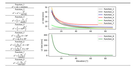
2.2. Weighting of Observation

Stochastic modeling is presented as VC matrix with variances population only and it depends on the use of the weighting functions. These weighting functions are related to the elevation angle.
Most of the existing software and studies use the trigonometric functions for weighting observations [58]. In this analysis, the seven weighting functions presented in Table 2 were chosen. First, the model where all observations have the same precision, without a function (hereinafter referred to as Function_1) was chosen. For all other cases, the precision of observations depends on the elevation angle. Function_2 was taken from AC MIT (GAMIT software) [59] and Function_3 from AC National Geodetic Survey (NGS) [58]. Function_4 is adopted from work [60]. Another way to weight observations is to use the threshold value of elevation angle, for example 30°, and to use different functions below and above this angle (Function_5 and Function_6), as was shown in works [11,32]. The final two functions are basic functions: the simple sine function (Function_7) [61] and square sine function (Function_8) [62]. All these weighting functions were implemented in the PPPH software used.
PPPH employs the adaptive robust EKF method, which introduces an equivalent weight matrix to compensate for the effect of outliers in observations, and also an adaptive factor to balance the contributions of measurement and estimated parameters [55]. In the Kalman filtering method, the functional model and relative dynamic model include the observation noise and process noise with a priori VC matrices, and both are considered to be Gaussian normal distribution (for optimal solutions). In the case of GNSS observation, such an assumption may be incorrect [63,64]. In our work, the a priori observation VC matrix is a diagonal matrix with variances for code and phase observations for GPS and Galileo observations. The initial uncertainty parameters were determined using the least squares estimation. In this method, the unknown parameters are estimated in the first epoch by the least squares adjustment, and then the estimated parameters and their statistical properties (which may be treated as estimators with Gaussian normal distribution) are utilized as the initial parameters for the next epoch.
For the calculations, both the pseudorange and carrier-phase observations with set precision of 0.2 m and 0.002 m for raw measurements [18,65] were used. Because the conventional PPP model uses an ionosphere-free linear combination, it causes a precision of 0.6 m and 0.006 m for the pseudorange and carrier-phase observations of this combination, respectively. Such precision was adopted for the G, E and GE solutions. The Galileo system is still in the phase of building, therefore in the case of the GE1 solution, the precision of 0.3 m and 0.003 m was set for the Galileo code and carrier-phase raw observations, respectively. For this solution, the precision of code and carrier-phase of Galileo observations for ionosphere-free linear combinations are 0.9 m and 0.009 m, respectively. This allowed for an analysis of how the GPS+Galileo solution would be affected by adopting a worse accuracy for Galileo observations.
The weighting functions used assume the precision of observations is the biggest at the zenith direction and decreases with lower elevation angles. For Function_1, Function_5, Function_6, Function_7 and Function_8, the precision of observation was set as mentioned above. Additionally, in Function_5, the precision of observations increases up to an elevation angle of 30°, and above this elevation angle, precision is the same for all observations. For Function_4, the value was adopted from [35].

2.3. Reference Coordinates
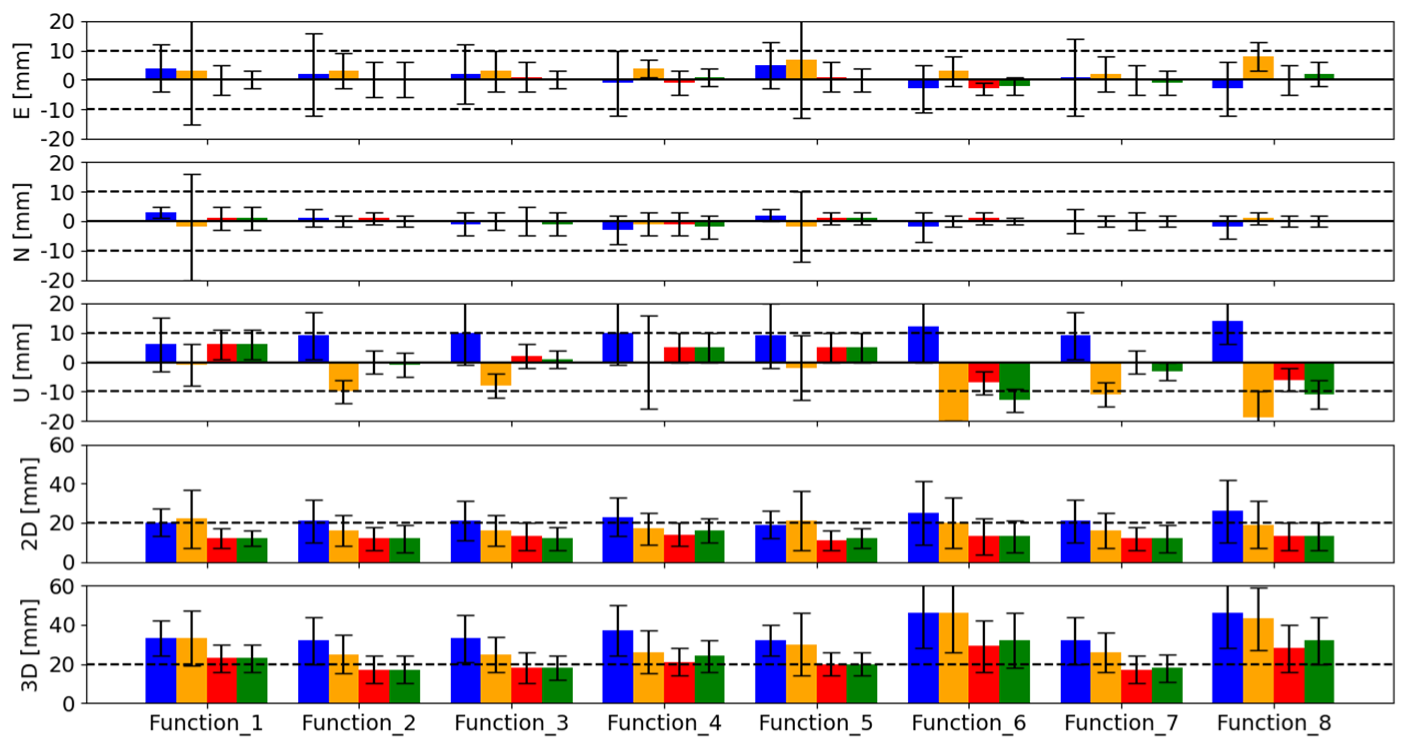
PPP quality assessment often focuses on accuracy and convergence time, which in turn strongly depends on the adoption of reference coordinates treated as ‘truth’. Additionally, in recent years, a significant development of multi-GNSS positioning is observed. Therefore, one of the most important goals of the MGEX project is to prepare products for official multi-GNSS-based combination solutions, which will be official IGS products in the future [66].
The multi-GNSS solutions computed by different ACs use different models than the official IGS, even for the same GNSS system [15,67]. There is already research on obtaining official combined solutions from all ACs, where discrepancies between different ACs are still obtained [13,14,15,67]. These differences are the consequences of using different models to determine the products, as well as the need to estimate parameters such as ISB [68] or using different receiver antenna models for Galileo observations [69,70]. Therefore, it is important to adopt appropriate reference coordinates in multi-GNSS analyzes.
Before beginning the principal analyses, we verified how the adopted reference coordinates affected the analyses performed (Figure A1). The following coordinates were calculated as reference coordinates: weekly from the G solution, weekly from the E solution and weekly from the GE solution, using the sine function as a function weighting the observations (Function_7). In addition, daily coordinates calculated by AC CNES/CLS from MGEX were also used. Any 3D errors were analyzed. From the obtained results, it can be seen that using only Galileo reference coordinates causes a bias of about 1 cm for GPS calculations. Also, the use of GPS reference coordinates produces a bias of approximately 1 cm for Galileo calculations. As shown in [69], the use of Galileo phase center corrections (PCC) models for Galileo observations causes a bias of -8 mm with respect to GPS results. The use of PCC GPS models for Galileo observations results in greater consistency of the results between Galileo and GPS solutions. For the results in relation to the daily reference coordinates calculated by AC CNES/CLS, the biggest errors were obtained for all analyzed solutions. The best results were obtained for reference coordinates calculated for weekly GPS+Galileo solutions, which eliminate systematic errors between GPS and Galileo. These coordinates are adopted as ‘truth’ coordinates, allowing the best possible analysis to be made.

3. Results

3.1. Detailed Analysis for MAS100ESP Station

In this subsection, results for only one station, MAS100ESP for 39 DoY, was presented. Similar analysis was performed for the rest of the stations but is not showed here. The MAS100ESP station was chosen as a station showing the average observation conditions for the Galileo system.
A minimum of 5 satellites from both the GPS and the Galileo systems were observed throughout the day. Most epochs had more GPS satellites observed, but there were some epochs with more Galileo satellites observed. On average, 9.9 of GPS satellites and 7.5 of Galileo satellites were observed. On average, 17.4 satellites using both systems were observed. When observing daily variations for PDOP, the PDOP value provided was more stable when both systems were used, unlike those of GPS-only or Galileo-only.
The signal strength (SNR) and multipath code combination (MP) for the Galileo E1 and E5a observations and for the GPS L1 and L2 observations was presented in Figure 2 and Figure 3, respectively. SNR for the Galileo observations are higher than the GPS observations, especially for E5a observations, which is higher than the L2 observations, with averages of 44.3 dBHz and 36.5 dBHz, respectively. The E1 observations have slightly lower SNR than the L1 observations, i.e., the SNR is 42.8 dBHz and 44.3 dBHz, respectively. We also noticed that Galileo observations, at lower elevation angles, have significantly higher SNR than GPS observations, due to the multipath effects (Figure 3) [71], whereas Galileo observations have higher performance with lower noise [20,72]. In addition, for L2 observations, it can be seen that some of the GPS satellites have a higher SNR. These satellites belong to the new satellite blocks (IIF and IIIA), which is in line with the goal of GPS modernization, i.e., improved accuracy, signal strength and observation quality [73].
In this study, the convergence time is described as the time when the station position reaches an accuracy of 20 cm and does not exceed this level thereafter. Figure 4 and Figure 5 present the time series of the first four hours for the Up component, horizontal (2D) and spatial (3D) errors for all analyzed weighting functions. The strong dependence of the error on used weighting functions is noticeable, especially for the first epochs. Moreover, the errors for the G and E have different behavior. For the E, the best results were obtained for Function_3, with 5 mm, 22 mm and 25 mm accuracy for the U component, 2D and 3D errors, respectively, whereas for the G, the best results were obtained for Function_7, with values of −1 mm, 10 mm and 16 mm, respectively. The shortest convergence time of 14 min was obtained for Function_8 for the E and 19 min was obtained for Function_7 for the G. In addition, for G, the slightly longer times were also obtained for Function_1, Function_2, Function_3 and Function_4. For the GE, the best results were obtained for Function_2, with 3 mm, 12 mm and 15 mm, respectively, and similarly for the GE1, with an accuracy of 3 mm, 13 mm and 16 mm, respectively. The best convergence time was obtained for Function_6, with 13 min for the GE, and for Function_1, Function_2 and Function_7, with 18 min for the GE1. For all cases, the GE1, where lower precision for Galileo observations was adopted, had worse results than the GE.
Based on the obtained results, it can be seen that the best results were obtained for Galileo-only (blue line) and the worst for GPS-only (orange line). The use of both systems together resulted in an improvement in the results relative to GPS-only. Also, the GE (red line), where the precision of observations was the same for both systems, showed more improvement than for the GE1 (green line), where for Galileo observations worse precision than GPS observations were accepted.
In the next step, we compared the estimated tropospheric delays with the IGS solutions. The results are presented in Figure 6. The worst results were obtained for the E for Function_6, where the average difference was −16.2 mm. The best solution for the E was obtained for Function_1, where the difference was −4.0 mm. Similar results were obtained for the G, where for Function_1 the best agreement with IGS solutions of 4.7 mm was also obtained. The worst, G, is based on Function_5, where a difference of 12.4 mm was obtained. In the other cases, the average difference did not exceed 10.0 mm. A systematic difference can be seen between the E and G, where it ranged from 8.7 mm for Function_7 to 24.3 mm for Function_6. Additionally, for the E, the results always showed negative values and positive values for the G.
GPS+Galileo solutions show much better compatibility with IGS solutions. It confirms the conclusion presented in [74] that using both systems together leads to better accuracy of ZPD. For both the GE and GE1, the mean differences did not exceed 6.5 mm, with the exception of the solutions based on Function_5 (for the GE and GE1) and Function_1 (for GE1), which all gave larger ZPD values than IGS. The highest consistency of the GE was obtained for Function_2, with a score of 0.4 mm, whereas for the GE1, Function_1 and Function_5 had a score of −1.0 mm. The worst results were obtained for Function_8, with 6.3 mm and 6.5 mm for the GE and GE1, respectively.
According to [75,76], the ISB parameter must be estimated for multi-GNSS positioning. ISB can be estimated as a constant value or as a time-varying value [67] and should have the same value regardless of the weighting functions. In our analysis, we estimated ISB as a random walk process. Figure 7 shows the estimated ISB for the analyzed GPS+Galileo solutions, where one can see the differences depending on the solution and the function used. For Function_1, for the GE, a big jump of around 14 h:30 min was observed. The difference for ISB was from −5.2 ns to −4.8 ns (about 11 cm), which did not occur for the GE1. For Function_6 (yellow) and Function_8 (gray) in the GE solution, a much worse consistency with the other weight functions was obtained after 19 h. The systematic difference was about 0.2 ns (6 cm). Changing the weights for the Galileo observations in the GE1 solution helped to remove this difference for Function_8, but, unfortunately, a discrepancy appeared between 15 h and 18 h. The other functions show a generally high consistency, in the range of 0.1 ns, which corresponds to less than 3 cm.

3.2. Overall Analysis

Using the individual results for all stations, such as the MAS100ESP example presented in the previous section, the mean values of the parameters discussed therein were determined. The following section presents the results for the obtained accuracies, convergence times, consistency of the obtained ZPD with the IGS solutions and ISB. In the examples analyzed, the average number of observed GPS satellites was on mean two more than the number of Galileo satellites, 7.6 and 9.5, respectively, and 17 satellites for both systems together.
An accuracy assessment for the East, North and Up components and for the horizontal (2D) and spatial (3D) errors was presented in Figure 8. The smallest errors were obtained for the North component. They did not exceed 3 mm for all solutions and weighting functions, with the exception of Function_1 and Function_5 for the G, where the results were consistent at all stations. The standard deviation was within 5 mm. For the two mentioned functions for the G, the standard deviation was 18 mm and 12 mm, respectively. The SUTM00ZAF station had an influence on the obtained results, for which significantly greater errors were obtained at −33 mm and −22 mm, respectively. No significant differences were observed on the northern component between the solutions (G, E, GE and GE1) and the weighting functions used.
Slightly larger errors were obtained for the East component, which strongly depends on the estimated ambiguities [77]. In general, they did not exceed 5 mm for all solutions and weighting functions. The exceptions are the Function_5 and Function_8 for the G. Their errors were 7 mm and 8 mm, respectively. The standard deviations of the mean errors are larger and range from 3 mm to 14 mm. Similarly, the largest deviations are for Function_1 and Function_5 for the G, and are 18 mm and 20 mm, respectively. For solutions based on the GPS+Galileo, the best results were obtained with an average value of 1 mm, with standard deviations ranging from 2 mm to 5 mm. The worst results were obtained for Function_2, in which the standard deviation amounted to 6 mm for both the GE and GE1. Reducing the precision of observations for Galileo (GE1) did not improve the results. Better statistics were obtained for the GE than for the GE1. The differences in results on the horizontal components are small. One could accept that the functions themselves do not really matter here, and if they do, it is only slightly for the GPS-only and Galileo-only solutions.
Significantly larger errors were obtained for the Up component. The positive values were always obtained for the E, whereas only the negative were for the G. A bias between the E and G was noted for all weighting functions. As shown in [69], using GPS receiver antenna phase center corrections for Galileo observations causes a bias of almost −8 mm for the Up component. In our solutions, the bias depends on the function used and varies from 7 mm for Function_1 to 38 mm for Function_6. A significant difference was also spotted for Function_8, at a value of 33 mm. For the remaining functions, they ranged between 10 and 20 mm. The standard deviation amounts were 10 mm for both the G and E. The best results, i.e., ±4 mm and ±8 mm for the G and E respectively, were obtained for Function_2 and Function_7. Much greater standard deviation was obtained for Function_4 for the G, which was ±16 mm. For the GE and GE1, better results were obtained than for the G and E, where the mean values were less than 7 mm, except for Function_6 and Function_8, for which the error values of −13 mm and −11 mm were obtained for the GE1. Standard deviation for the GE and GE1 was less than 5 mm for all functions.
Regarding the 2D error, in case of the E, values of about 20 mm were obtained with a standard deviation of 10 mm, except for Function_6 and Function_8, for which 25 mm and 26 mm were obtained with a standard deviation of 16 mm, respectively. For the G, the values were 16–17 mm for Function_2, Function_3, Function_4 and Function_7, with standard deviations of 8–9 mm, whereas for the remaining functions, the values reached 19–22 mm, with standard deviations of 12–15 mm. In case of the GE and GE1, the values amounted to 12–13 mm, with standard deviations of 4–7 mm for all weighting functions, except Function_4 for which errors of 16 mm and 14 mm were obtained, respectively. For the GE1 and GE, and Function_6, standard deviations of 8 mm and 9 mm were obtained.
Regarding the analysis for the 3D error, lower values were obtained for the G than for the E. The accuracy for the G amounted 25–33 mm with a standard deviation of approximately 10 mm, except for Function_6 and Function_8, for which the values of 43 mm and 46 mm were obtained with a standard deviation of 20 mm and 16 mm, respectively. The best values were obtained for Function_3, i.e., 26 ± 9 mm. For the E, the error values ranged from 32–37, mm with a standard deviation of approximately 10 mm. Again, the worst results were obtained for Function_6 and Function_8, with 46 ± 18 mm. On the other hand, the best results were obtained for Function_5, i.e., 32 ± 8 mm. For the GE and GE1, better results were obtained than for the G and E. The error values ranged from 17–23 mm wit standard deviations of 6–8 mm. Additionally, for these solutions, the worst values were obtained for Function_6 and Function_8. In case of the GE1, they amounted to 32 ± 14 mm and 32 ± 12 mm, whereas for the GE, they amounted to 29 ± 13 mm and 28 ± 12 mm. The best values for both solutions were obtained for Function_2 17 ± 7 mm.
The use of different weighting functions was reflected most for the Up component. The best results for the G were obtained by applying Function_3, whereas for the E, the best results were obtained for Function_5. For all solutions (i.e., G, E, GE, GE1), the worst accuracies were obtained with Function_6 and Function_8. Likewise, it can be noted that slightly larger errors were obtained for the GE1 than for GE, confirming that the Galileo system already allows for achieving similar accuracy to the GPS. Thus, defining lower weights for Galileo observations is not necessary.
Figure 9 shows the results of the convergence time analysis. The best results were obtained for the North component, where it was below 16 min in most cases. In case of the East component, convergence time was below 20 min in most cases. For the horizontal components, the advantage of Galileo solutions over GPS solutions can be seen. The convergence time is on average 3 min (about 15%) shorter. It is an opposite situation for the vertical component, where GPS solutions gave better results than Galileo. The convergence time here is comparable to the values obtained for the eastern component, which was less than 20 min, except for Function_4, Function_6 and Function_8, where it was 20 min and 22 min; 24 min and 24 min; and 28 min and 24 min, for the E and G, respectively. For the Up component, there is a clear improvement for GPS+Galileo solutions compared to GPS-only and Galileo-only.
The total effect of all components (East, North and Up) is presented in the analysis for the 3D error, for which the convergence time in all solutions very much depends on the weighting functions used. For the E, the shortest convergence time was obtained for Function_5, being 36 ± 16 min. In contrast, the longest convergence time was obtained for Function_8, amounting to 69 ± 54 min. For the G, the shortest convergence time was obtained for Function_3, which equaled 36 ± 22 min. In turn, the longest convergence time was obtained for Function_6. It amounted to 59 ± 44 min. For the GE and GE1, the shortest convergence time was obtained for Function_5, i.e., approximately 21 ± 5 min for the GE and 22 ± 6 min for the GE1. Similar results were obtained for Function_2, which was only less than a minute longer. For both the GE and GE1, the longest convergence time was obtained for Function_6 and Function_8, amounting to 34 ± 23 min and 30 ± 20 min, respectively. Reusing the two systems together resulted in a shorter convergence time than for each system separately and a shorter convergence time for the GE than that for the GE1 was obtained.
When comparing analysis of the convergence time with the accuracy, it can be seen that the use of different weight functions in addition to the Up component also affects the East component.
Figure 10 shows the results of the ZPD tests. The best values for all solutions were obtained for the E. Then, slightly worse results were obtained for the GE and GE1, and the worst values were obtained for the G. For most solutions and weighting functions, the error values and standard deviation are less than 10 mm. The exception is Function_6 and Function_8. For these functions in solution E, a mean difference of less than 0.5 mm was obtained. However, the scatter of the results is large, as evidenced by the high value of the standard deviation—14 mm and 16 mm for Function_6 and Function_8, respectively. In addition, for the G for Function_1 and Function_5, the standard deviation was greater than 10 mm and amounted to 12.2 mm and 11.1 mm, respectively.
For the E, the accuracy of about 2-3 mm was obtained with the best recorded values for Function_5 being 2.5 ± 8.6 mm. For the G, the accuracy ranged from 6 to 9 mm, with the best values for Function_3 being 8.2 ± 7.4 mm. In case of the GE and GE1, the accuracy ranged from 5 to 7 mm, with better values for the GE than for the GE1. For these above solutions, the best values were obtained for Function_4, for which 4.7 ± 6.9 mm and 5.1 ± 6.2 mm were obtained, respectively.
ISB obtained from the GE and GE1 (not showed here) were also analyzed. For this purpose, ISB were averaged and standard deviations were calculated for all stations of each type of receiver model (Table A1) from the analyzed period. Based on the obtained results, there was no correlation with the weighting functions used. The maximum difference between the functions was 3 cm, but with different dependencies for each type of receiver. Additionally, between the GE and GE1, the maximum differences were less than 2 cm and have no dependencies with the used functions. For a more detailed analyses related to the use of different weighting functions and ISB, it will be required to perform analyses for more receiver types and to use a greater number of stations for each type of receiver.

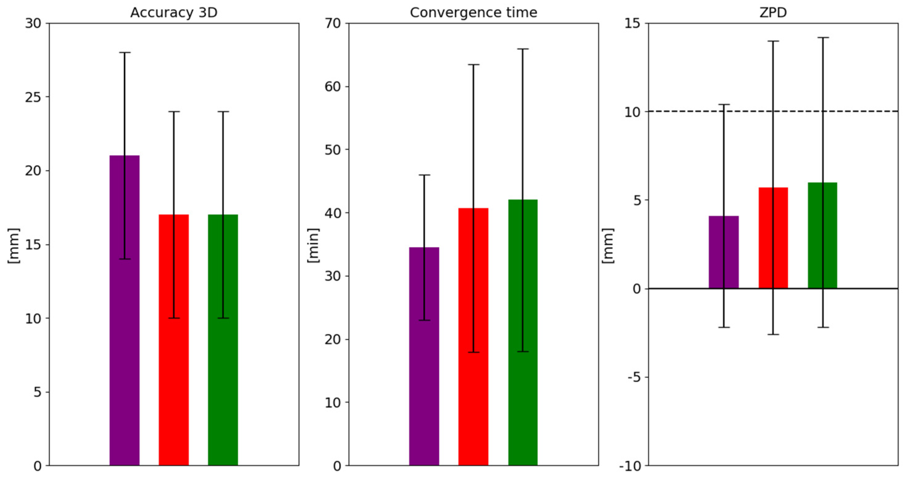
4. Proposed Approach for GPS+Galileo Solution

For the G and E, the best results were obtained for Function_3 and Function_5, respectively. Therefore, a new observation weighting approach for the GPS+Galileo positioning was proposed. It uses different weighting functions for both systems. For this new solution, named GE_new, Function_3 was used for GPS and Function_5 for Galileo. This solution used the same precision of GPS and Galileo observations as the GE solution. The results of this solution were compared with the results obtained for the GE and GE1 for Function_2, for which the best results were obtained. The results are shown in Figure 11.
For the GE_new, the obtained 3D accuracy was inferior compared to the GE and GE1. The accuracy for the GE_new was 21 ± 7 mm, whereas for the GE and GE1 it was 17 ± 7 mm. However, when analyzing the convergence time and ZPD, an improvement was achieved. For the GE_new, the convergence time was 21 ± 5 min, whereas for the GE and GE1 it was 24 ± 13 min and 22 ± 10 min, respectively. The significantly smaller standard deviation is particularly noticeable here. When analyzing ZPD for the GE_new, a value of 4.1 ± 6.3 mm was obtained, whereas the values for the GE and GE1 were 5.7 ± 8.3 mm and 6.0 ± 8.2 mm, respectively.
Adopting two different weighting functions for GPS+Galileo solutions, separately for each system, gave better results than using the same function for both systems. In addition, in the literature [33,38], it was shown that using different weighting methods for different systems gave better results. The obtained positioning accuracy was worse, but only by 4 mm. On the other hand, a shorter convergence time and higher accuracy of the estimated ZPD were obtained, particularly with a smaller standard deviation. An improvement of about 5% was obtained for the convergence time and about 30% for the tropospheric delay.

5. Discussion and Conclusions

In order to obtain better GNSS positioning results, as in any geodetic process, observations should be weighted according to the measurement errors made. The simplest method is to weigh the observations by the elevation angle using a simple sine function [78]. In this study, the impact of different weighting functions on the performance of PPP for GPS, Galileo and GPS+Galileo was analyzed. Eight models have been selected for analysis: one of them assumes that all observations have the same precision, without dependence on the elevation angle; for the rest, selected elevation-dependent functions were used. In this paper, parameters that related to the quality of PPP solutions such as accuracy, convergence time, ZPD and ISB are analyzed.
The results showed that for different solutions, different functions allowed for obtaining the best results. It is worth emphasizing that the weighting functions have the biggest impact for the Up component. This concerns the accuracy and convergence time. Additionally in convergence time, using different weighting functions also has an impact on the East component.
For GPS-only, the highest accuracy was obtained for the Function_3, whereas for Galileo-only, the best result was obtained for Function_5. Both functions depend on the elevation angle, but for Function_3, the errors for lower satellites have less weight (Figure 12). This is different for Function_5, where observations at lower angles have more weight relative to most other functions. With higher signal strength and less multipath effect for low Galileo satellites, this improves Galileo-only solutions. It is worth noting that GPS observations from the newest satellites also have higher signal strength and less multipath effect, so it will be worthwhile to do the study again in the future for GPS, where the vast majority of satellites will be newer generation.
For GPS+Galileo, we analyzed two solutions. The first one used the same precision of observations for GPS and Galileo (GE solution). The second one (GE1) used a slightly lower precision for Galileo observations. Unlike the GPS-only and Galileo-only solutions, for the GE and GE1 solutions, the best accuracy were obtained for the same functions—Function_2. The shortest convergence time was obtained for Function_5. Considering that the difference in convergence time between Function_2 and Function_5 is less than a minute, it should be pointed out that the Function_2 proved to be the best. The accuracy for the GE solution was found to be better than that for the GE1.
The worst results were obtained for Function_6 and Function_8. The solutions were even worse than the solution without weights (Function_1). Both functions give very low weights to low observations, an order of magnitude lower than for the other models analyzed. This directly translated into the worst result obtained. This shows that improper weighting of observations can degrade the results.
The best agreement of the tropospheric solutions with the IGS solutions was obtained for the Galileo-only solution. Slightly worse results were obtained for the GPS+Galileo solutions and the worst were for the GPS-only. As shown, the weighting functions have an influence on the results obtained. For the Galileo-only solution, the best results were obtained for Function_5, whereas for the G-only solutions, the best results were obtained for Function_3, similar to accuracy and convergence time. For the GPS+Galielo solutions, the best results were obtained for Function_4, and again better results were for the GE solution than for the GE1 solution.
When analyzing the ISB parameter, there was no significant dependence on the weighting functions used. Further research on a statistically larger sample of receivers is needed to document a reliable impact.
A new approach was proposed for the final analysis. The best functions for GPS (Function_3) and Galileo (Function_5) were used separately for those systems in the GPS+Galileo solution. The obtained results were compared with results of the GE and GE1 solutions, for which the best results were obtained for the same as Function_2. Although the positioning accuracy was worse by 4 mm, other parameters (convergence time and troposphere) performed much better. The lower accuracy may be due to the fact that there is still an advantage of GPS satellites over Galileo. GPS has a complete constellation of satellites evenly spaced across all orbits, resulting in more satellites available with better geometry than Galileo [79]. This results in a greater influence of GPS on the results obtained. The proposed approach increases the weight of the Galileo observations, especially for low observations (Figure 12). With still slightly less accurate products for Galileo, this results in a decrease in the accuracy obtained. However, it should be noted that the decrease in accuracy is small. If we consider that significantly improved convergence time and obtained higher accuracy of the estimated ZPD, it should be concluded that in general the proposed approach based on different functions for two systems gives better results.
In conclusion, it should be noted that Galileo achieves similar accuracy as GPS. Therefore, at least the same observation accuracy for both systems can be assumed for GPS+Galileo positioning. There is no reason to reduce the accuracy of the latest Galileo observations relative to GPS. Considering that each system has different characteristics, different weighting functions of observations should be used. The conducted analyzes of the weighting function clearly show it. As Galileo observations at lower elevation angles perform better than GPS, they should be given more weight than GPS observations.
The conducted analyzes require further studies, which are planned for the future. Research on stochastic modeling will be extended to the variance components analysis, e.g., using the LS-VCE method.

Author Contributions

Conceptualization, D.K.; Methodology, D.K.; Software, D.K.; Validation, D.K., K.K. and A.A.; Formal analysis, D.K.; Investigation, D.K.; Writing—original draft preparation, D.K.; Writing—review and editing, K.K. and A.A.; Visualization, D.K. All authors have read and agreed to the published version of the manuscript.

Funding

This research was funded by the Military University of Technology in Warsaw, Faculty of Civil Engineering and Geodesy, Institute of Geospatial Engineering and Geodesy statutory research funds UGB/22-785/2022/WAT.

Data Availability Statement

All used data in this study are collected by IGS, which can be obtained from IGS data centers.

Conflicts of Interest

The authors declare no conflict of interest.

Appendix A

Figure A1. Analyzed the impact of different reference coordinates for obtained accuracy. Blue—weekly reference coordinates from E solution, orange—weekly reference coordinates from G solution, red—weekly reference coordinates from GE solution and green—daily reference coordinates from AC CNES/CLS.
Remotesensing 14 02223 g0a1
Table A1. Types of receiver and antenna mounted on stations selected for analysis, together with a list of external clocks and date of the latest changed receiver.
StationReceiverClockDate of the Latest Changed Receiver
SUTM00ZAFJAVAD TRE_3INTERNAL10.05.2019
ULAB00MNGJAVAD TRE_3INTERNAL20.09.2018
BOGT00COLJAVAD TRE_3 DELTAINTERNAL19.08.2015
TRO100NORTRIMBLE NETR9EXTERNAL RUBIDIUM30.06.2017
UCAL00CANTRIMBLE NETR9INTERNAL21.08.2013
CCJ200JPNTRIMBLE NETR9INTERNAL22.02.2012
NKLG00GABSEPT POLARX5INTERNAL21.08.2019
MAS100ESPSEPT POLARX5EXTERNAL CESIUM15.10.2019
MGUE00ARGSEPT POLARX5TREXTERNAL H-MASER29.04.2019
BRUX00BELSEPT POLARX5TREXTERNAL CH1-75A MASER25.02.2020
NNOR00AUSSEPT POLARX5TREXTERNAL SLAVED CRYSTAL25.10.2019
NICO00CYPLEICA GR50INTERNAL08.11.2019
REYK00ISLLEICA GR50INTERNAL14.05.2019

References

  1. Kouba, J.; Lahaye, F.; Tétreault, P. Precise Point Positioning. In Springer Handbook of Global Navigation Satellite Systems; Teunissen, P.J.G., Montenbruck, O., Eds.; Springer International Publishing: Cham, Switzerland, 2017; p. 723. [Google Scholar]
  2. Héroux, P.; Kouba, J. GPS Precise Point Positioning with a Difference; Natural Resources Canada, Geomatics Canada, Geodetic Survey Division: Ottawa, ON, Canada, 1995.
  3. Malys, S.; Jensen, P.A. Geodetic Point Positioning with GPS Carrier Beat Phase Data from the CASA UNO Experiment. In Geophysical Research Letters; John Wiley & Sons, Ltd.: Hoboken, NJ, USA, 1990; Volume 17, pp. 651–654. [Google Scholar]
  4. Zumberge, J.F.; Heflin, M.B.; Jefferson, D.C.; Watkins, M.M.; Webb, F.H. Precise Point Positioning for the Efficient and Robust Analysis of GPS Data from Large Networks. J. Geophys. Res. Solid Earth 1997, 102, 5005–5017. [Google Scholar] [CrossRef] [Green Version]
  5. Héroux, P.; Kouba, J. GPS Precise Point Positioning Using IGS Orbit Products. Phys. Chem. Earth Part A Solid Earth Geod. 2001, 26, 573–578. [Google Scholar] [CrossRef]
  6. Kouba, J.; Springer, T. New IGS Station and Satellite Clock Combination. GPS Solut. 2001, 4, 31–36. [Google Scholar] [CrossRef]
  7. Cai, C.; Gao, Y. Precise Point Positioning Using Combined GPS and GLONASS Observations. J. Glob. Position. Syst. 2007, 6, 13–22. [Google Scholar] [CrossRef] [Green Version]
  8. Tegedor, J.; Øvstedal, O.; Vigen, E. Precise Orbit Determination and Point Positioning Using GPS, Glonass, Galileo and BeiDou. J. Geod. Sci. 2014, 4, 65–73. [Google Scholar] [CrossRef] [Green Version]
  9. Li, X.; Liu, G.; Li, X.; Zhou, F.; Feng, G.; Yuan, Y.; Zhang, K. Galileo PPP Rapid Ambiguity Resolution with Five-Frequency Observations. GPS Solut. 2019, 24, 24. [Google Scholar] [CrossRef]
  10. Su, K.; Jin, S. Analytical Performance and Validations of the Galileo Five-Frequency Precise Point Positioning Models. Measurement 2021, 172, 108890. [Google Scholar] [CrossRef]
  11. Guo, J.; Geng, J.; Wang, C. Impact of the Third Frequency GNSS Pseudorange and Carrier Phase Observations on Rapid PPP Convergences. GPS Solut. 2021, 25, 30. [Google Scholar] [CrossRef]
  12. Geng, J.; Pan, Y.; Yang, S.; Li, P.; Geng, J.; Pan, Y.; Yang, S.; Li, P. Combining Multi-GNSS Phase Bias Products for Improved Undifferenced Ambiguity Resolution. In Proceedings of the EGU General Assembly Conference Abstracts, Online, 19–30 April 2021; p. EGU21-2531. [Google Scholar]
  13. Mansur, G.; Sakic, P.; Männel, B.; Schuh, H. Multi-Constellation GNSS Orbit Combination Based on MGEX Products. Adv. Geosci. 2020, 50, 57–64. [Google Scholar] [CrossRef] [Green Version]
  14. Sośnica, K.; Zajdel, R.; Bury, G.; Bosy, J.; Moore, M.; Masoumi, S. Quality Assessment of Experimental IGS Multi-GNSS Combined Orbits. GPS Solut. 2020, 24, 54. [Google Scholar] [CrossRef] [Green Version]
  15. Steigenberger, P.; Montenbruck, O. Consistency of MGEX Orbit and Clock Products. Engineering 2020, 6, 898–903. [Google Scholar] [CrossRef]
  16. Su, K.; Jin, S.; Jiao, G. Assessment of Multi-Frequency Global Navigation Satellite System Precise Point Positioning Models Using GPS, BeiDou, GLONASS, Galileo and QZSS. Meas. Sci. Technol. 2020, 31, 064008. [Google Scholar] [CrossRef]
  17. Ogutcu, S. Assessing the Contribution of Galileo to GPS+GLONASS PPP: Towards Full Operational Capability. Measurement 2020, 151, 107143. [Google Scholar] [CrossRef]
  18. Hofmann-Wellenhof, B.; Lichtenegger, H.; Wasle, E. GNSS—Global Navigation Satellite Systems. GPS, GLONASS, Galileo, and More; Springer: Vienna, Austria, 2008; ISBN 978-3-211-73012-6. [Google Scholar]
  19. Luo, X. GPS Stochastic Modelling: Signal Quality Measures and ARMA Processes; Springer Theses: Berlin, Germany; Springer Science & Business Media: Berlin/Heidelberg, Germany, 2013; ISBN 978-3-642-34835-8. [Google Scholar]
  20. Prochniewicz, D.; Wezka, K.; Kozuchowska, J. Empirical Stochastic Model of Multi-GNSS Measurements. Sensors 2021, 21, 4566. [Google Scholar] [CrossRef]
  21. Tiberius, C.C.J.M.; Kenselaar, F. Estimation of the Stochastic Model for GPS Code and Phase Observables. Surv. Rev. 2000, 35, 441–454. [Google Scholar] [CrossRef]
  22. Wang, J.-G.; Gopaul, N.; Scherzinger, B. Simplified Algorithms of Variance Component Estimation for Static and Kinematic GPS Single Point Positioning. J. Glob. Position. Syst. 2009, 8, 43–52. [Google Scholar] [CrossRef]
  23. Teunissen, P.J.G.; Amiri-Simkooei, A.R. Least-Squares Variance Component Estimation. J. Geod. 2007, 82, 65–82. [Google Scholar] [CrossRef] [Green Version]
  24. Amiri-Simkooei, A.R.; Teunissen, P.J.G.; Tiberius, C.C.J.M. Application of Least-Squares Variance Component Estimation to GPS Observables. J. Surv. Eng. 2009, 135, 149–160. [Google Scholar] [CrossRef] [Green Version]
  25. Zhang, X.; Li, P.; Tu, R.; Lu, X.; Ge, M.; Schuh, H. Automatic Calibration of Process Noise Matrix and Measurement Noise Covariance for Multi-GNSS Precise Point Positioning. Mathematics 2020, 8, 502. [Google Scholar] [CrossRef] [Green Version]
  26. Mirmohammadian, F.; Asgari, J.; Verhagen, S.; Amiri-Simkooei, A. Improvement of Multi-GNSS Precision and Success Rate Using Realistic Stochastic Model of Observations. Remote Sens. 2021, 14, 60. [Google Scholar] [CrossRef]
  27. Hou, P.; Zha, J.; Liu, T.; Zhang, B. LS-VCE Applied to Stochastic Modeling of GNSS Observation Noise and Process Noise. Remote Sens. 2022, 14, 258. [Google Scholar] [CrossRef]
  28. [IGSMAIL-1569] IGS Workshop, GB Meeting 1997 in Pasadena. Available online: https://lists.igs.org/pipermail/igsmail/1997/002941.html (accessed on 8 April 2022).
  29. [IGSMAIL-1586] Elevation Cut-Off Angle. Available online: https://lists.igs.org/pipermail/igsmail/1997/002958.html (accessed on 8 April 2022).
  30. [IGSMAIL-1705] CODE Analysis Changes. Available online: https://lists.igs.org/pipermail/igsmail/1997/003077.html (accessed on 8 April 2022).
  31. Gao, C.; Wu, F.; Chen, W.; Wang, W. An Improved Weight Stochastic Model in GPS Precise Point Positioning. In Proceedings of the 2011 International Conference on Transportation, Mechanical, and Electrical Engineering, TMEE, Changchun, China, 16–18 December 2011; pp. 629–632. [Google Scholar] [CrossRef]
  32. Yu, X.; Gao, J. Kinematic Precise Point Positioning Using Multi-Constellation Global Navigation Satellite System (GNSS) Observations. ISPRS Int. J. Geo-Inf. 2017, 6, 6. [Google Scholar] [CrossRef] [Green Version]
  33. Kazmierski, K.; Hadas, T.; Sośnica, K. Weighting of Multi-GNSS Observations in Real-Time Precise Point Positioning. Remote Sens. 2018, 10, 84. [Google Scholar] [CrossRef] [Green Version]
  34. Liu, T.; Wang, J.; Yu, H.; Cao, X.; Ge, Y. A New Weighting Approach with Application to Ionospheric Delay Constraint for GPS/GALILEO Real-Time Precise Point Positioning. Appl. Sci. 2018, 8, 2537. [Google Scholar] [CrossRef] [Green Version]
  35. Kiliszek, D.; Szołucha, M.; Kroszczyński, K. Accuracy of Precise Point Positioning (PPP) with the Use of Different International GNSS Service (IGS) Products and Stochastic Modelling. Geod. Cartogr. 2018, 67, 207–238. [Google Scholar] [CrossRef]
  36. Jiang, N.; Xu, T.; Xu, Y.; Xu, G.; Schuh, H. Assessment of Different Stochastic Models for Inter-System Bias between GPS and BDS. Remote Sens. 2019, 11, 989. [Google Scholar] [CrossRef] [Green Version]
  37. Zhang, Q.; Zhao, L.; Zhou, J. A Weighting Method for Code and Phase Observations in Precise Point Positioning. In Proceedings of the 2018 IEEE CSAA Guidance, Navigation and Control Conference, CGNCC, Xiamen, China, 10–12 August 2018. [Google Scholar] [CrossRef]
  38. Pan, L.; Gao, X.; Hu, J.; Ma, F.; Zhang, Z.; Wu, W. Performance Assessment of Real-Time Multi-GNSS Integrated PPP with Uncombined and Ionospheric-Free Combined Observables. Adv. Space Res. 2021, 67, 234–252. [Google Scholar] [CrossRef]
  39. Constellation Information|European GNSS Service Centre. Available online: https://www.gsc-europa.eu/system-service-status/constellation-information (accessed on 8 April 2022).
  40. Hadas, T.; Kazmierski, K.; Sośnica, K. Performance of Galileo-Only Dual-Frequency Absolute Positioning Using the Fully Serviceable Galileo Constellation. GPS Solut. 2019, 23, 108. [Google Scholar] [CrossRef] [Green Version]
  41. Kiliszek, D.; Kroszczyński, K. Performance of the Precise Point Positioning Method along with the Development of GPS, GLONASS and Galileo Systems. Measurement 2020, 164, 108009. [Google Scholar] [CrossRef]
  42. Douša, J.; Václavovic, P.; Kala, M.; Bezděka, P.; Zhao, L. GOP Contribution to Independent Monitoring of Galileo OS Navigation Performance; VSB—Technical University of Ostrava: Ostrava, Czechia, 2021. [Google Scholar]
  43. Carlin, L.; Hauschild, A.; Montenbruck, O. Precise Point Positioning with GPS and Galileo Broadcast Ephemerides. GPS Solut. 2021, 25, 77. [Google Scholar] [CrossRef]
  44. Caporali, A.; Zurutuza, J.; Paziewski, J.; Li, X. Broadcast Ephemeris with Centimetric Accuracy: Test Results for GPS, Galileo, Beidou and Glonass. Remote Sens. 2021, 13, 4185. [Google Scholar] [CrossRef]
  45. Liu, T.; Chen, H.; Chen, Q.; Jiang, W.; Laurichesse, D.; An, X.; Geng, T. Characteristics of Phase Bias from CNES and Its Application in Multi-Frequency and Multi-GNSS Precise Point Positioning with Ambiguity Resolution. GPS Solut. 2021, 25, 58. [Google Scholar] [CrossRef]
  46. Geng, J.; Guo, J.; Meng, X.; Gao, K. Speeding up PPP Ambiguity Resolution Using Triple-Frequency GPS/BeiDou/Galileo/QZSS Data. J. Geod. 2020, 94, 6. [Google Scholar] [CrossRef] [Green Version]
  47. Glaner, M.; Weber, R. PPP with Integer Ambiguity Resolution for GPS and Galileo Using Satellite Products from Different Analysis Centers. GPS Solut. 2021, 25, 102. [Google Scholar] [CrossRef]
  48. Duan, B.; Hugentobler, U.; Selmke, I.; Wang, N. Estimating Ambiguity Fixed Satellite Orbit, Integer Clock and Daily Bias Products for GPS L1/L2, L1/L5 and Galileo E1/E5a, E1/E5b Signals. J. Geod. 2021, 95, 44. [Google Scholar] [CrossRef]
  49. Schaer, S.; Villiger, A.; Arnold, D.; Dach, R.; Prange, L.; Jäggi, A. The CODE Ambiguity-Fixed Clock and Phase Bias Analysis Products: Generation, Properties, and Performance. J. Geod. 2021, 95, 81. [Google Scholar] [CrossRef]
  50. Zhao, L.; Blunt, P.; Yang, L. Performance Analysis of Zero-Difference GPS L1/L2/L5 and Galileo E1/E5a/E5b/E6 Point Positioning Using CNES Uncombined Bias Products. Remote Sens. 2022, 14, 650. [Google Scholar] [CrossRef]
  51. Guo, J.; Zhang, Q.; Li, G.; Zhang, K. Assessment of Multi-Frequency PPP Ambiguity Resolution Using Galileo and BeiDou-3 Signals. Remote Sens. 2021, 13, 4746. [Google Scholar] [CrossRef]
  52. Banville, S.; Geng, J.; Loyer, S.; Schaer, S.; Springer, T.; Strasser, S. On the Interoperability of IGS Products for Precise Point Positioning with Ambiguity Resolution. J. Geod. 2020, 94, 10. [Google Scholar] [CrossRef]
  53. MGEX Product Analysis—International GNSS Service. Available online: https://igs.org/mgex/analysis/ (accessed on 8 April 2022).
  54. Kp-Index. Available online: https://www.gfz-potsdam.de/kp-index/ (accessed on 8 April 2022).
  55. Bahadur, B.; Nohutcu, M. PPPH: A MATLAB-Based Software for Multi-GNSS Precise Point Positioning Analysis. GPS Solut. 2018, 22, 113. [Google Scholar] [CrossRef]
  56. Kouba, J. A Guide to Using International GNSS Service (IGS) Products; Geodetic Survey Division Natural Resources Canada Ottawa: Ottawa, ON, Canada, 2015.
  57. Petit, G.; Brian, L. IERS Conventions; Bureau International des Poids et Mesures Sevres (France): Saint-Cloud, France, 2010. [Google Scholar]
  58. Ray, J.; Griffiths, J. Overview of IGS Products and Analysis Center Modeling. In Proceedings of the IGS Analysis Center Workshop, Miami Beach, FL, USA, 2–6 June 2008. [Google Scholar]
  59. Herring, T.A.; King, R.W.; Floyd, M.A.; McClusky, S.C. Documentation for the GAMIT GPS Analysis Software 10.70; MIT: Cambridge, MA, USA, 2018. [Google Scholar]
  60. Jin, X.X.; de Jong, C.D. Relationship Between Satellite Elevation and Precision of GPS Code Observations. J. Navig. 1996, 49, 253–265. [Google Scholar] [CrossRef]
  61. Rothacher, M.; Springer, T.A.; Schaer, S.; Beutler, G. Processing Strategies for Regional GPS Networks. In Proceedings of the IAG General Assembly 1997, Rio de Janeiro, Brazil, 2–13 July 1997; Brunner, F.K., Ed.; Springer: Berlin/Heidelberg, Germany; New York, NY, USA, 1998; pp. 93–100. [Google Scholar]
  62. ÖZLÜDEMİR, M.T. The Stochastic Modeling of GPS Observations. Turk. J. Eng. Environ. Sci. 2004, 28, 223–231. [Google Scholar] [CrossRef]
  63. Tiberius, C.C.J.M.; Borre, K. Are GPS Data Normally Distributed. In Geodesy Beyond; Springer: Berlin/Heidelberg, Germany, 2000; pp. 243–248. [Google Scholar] [CrossRef]
  64. Luo, X.; Mayer, M.; Heck, B. On the Probability Distribution of GNSS Carrier Phase Observations. GPS Solut. 2010, 15, 369–379. [Google Scholar] [CrossRef]
  65. Paziewski, J.; Sieradzki, R.; Wielgosz, P. On the Applicability of Galileo FOC Satellites with Incorrect Highly Eccentric Orbits: An Evaluation of Instantaneous Medium-Range Positioning. Remote Sens. 2018, 10, 208. [Google Scholar] [CrossRef] [Green Version]
  66. Montenbruck, O.; Steigenberger, P.; Prange, L.; Deng, Z.; Zhao, Q.; Perosanz, F.; Romero, I.; Noll, C.; Stürze, A.; Weber, G.; et al. The Multi-GNSS Experiment (MGEX) of the International GNSS Service (IGS)—Achievements, Prospects and Challenges. Adv. Space Res. 2017, 59, 1671–1697. [Google Scholar] [CrossRef]
  67. Sakic, P.; Mansur, G.; Viegas, E.; Männel, B.; Schuh, H. Towards a Multi-Constellation Combination: Improving the IGS Orbit and Clock Combination Software for MGEX Products. In Proceedings of the IGS Workshop, Wuhan, China, 19–21 March 2018. [Google Scholar]
  68. Paziewski, J.; Wielgosz, P. Assessment of GPS+Galileo and Multi-Frequency Galileo Single-Epoch Precise Positioning with Network Corrections. GPS Solut. 2013, 18, 571–579. [Google Scholar] [CrossRef] [Green Version]
  69. Araszkiewicz, A.; Kiliszek, D. Impact of Using GPS L2 Receiver Antenna Corrections for the Galileo E5a Frequency on Position Estimates. Sensors 2020, 20, 5536. [Google Scholar] [CrossRef]
  70. Villiger, A.; Dach, R.; Schaer, S.; Prange, L.; Zimmermann, F.; Kuhlmann, H.; Wübbena, G.; Schmitz, M.; Beutler, G.; Jäggi, A. GNSS Scale Determination Using Calibrated Receiver and Galileo Satellite Antenna Patterns. J. Geod. 2020, 94, 93. [Google Scholar] [CrossRef]
  71. Xia, F.; Ye, S.; Xia, P.; Zhao, L.; Jiang, N.; Chen, D.; Hu, G. Assessing the Latest Performance of Galileo-Only PPP and the Contribution of Galileo to Multi-GNSS PPP. Adv. Space Res. 2019, 63, 2784–2795. [Google Scholar] [CrossRef]
  72. Tian, Y.; Sui, L.; Xiao, G.; Zhao, D.; Tian, Y. Analysis of Galileo/BDS/GPS Signals and RTK Performance. GPS Solut. 2019, 23, 37. [Google Scholar] [CrossRef]
  73. GPS.Gov: Space Segment. Available online: https://www.gps.gov/systems/gps/space/#generation (accessed on 8 April 2022).
  74. Hadas, T.; Hobiger, T. Benefits of Using Galileo for Real-Time GNSS Meteorology. IEEE Geosci. Remote Sens. Lett. 2020, 18, 1756–1760. [Google Scholar] [CrossRef]
  75. Hong, J.; Tu, R.; Gao, Y.; Zhang, R.; Fan, L.; Zhang, P.; Liu, J. Characteristics of Inter-System Biases in Multi-GNSS with Precise Point Positioning. Adv. Space Res. 2019, 63, 3777–3794. [Google Scholar] [CrossRef]
  76. Paziewski, J.; Sieradzki, R.; Wielgosz, P. Selected Properties of GPS and Galileo-IOV Receiver Intersystem Biases in Multi-GNSS Data Processing. Meas. Sci. Technol. 2015, 26, 095008. [Google Scholar] [CrossRef]
  77. Ge, M.; Gendt, G.; Rothacher, M.; Shi, C.; Liu, J. Resolution of GPS Carrier-Phase Ambiguities in Precise Point Positioning (PPP) with Daily Observations. J. Geod. 2007, 82, 389–399. [Google Scholar] [CrossRef]
  78. Satirapod, C.; Luansang, M. Comparing Stochastic Models Used in GPS Precise Point Positioning Technique. Surv. Rev. 2013, 40, 188–194. [Google Scholar] [CrossRef]
  79. Zhang, Z.; Pan, L. Current Performance of Open Position Service with Almost Fully Deployed Multi-GNSS Constellations: GPS, GLONASS, Galileo, BDS-2, and BDS-3. Adv. Space Res. 2022, 69, 1994–2019. [Google Scholar] [CrossRef]
Figure 1. Location of test stations.
Remotesensing 14 02223 g001
Figure 2. Signal to noise ratio (SNR) for the E1 and E5a observations for the Galileo and L1 and L2 observations for the GPS for the MAS100ESP station for the 39 DoY with function of elevation angle.
Remotesensing 14 02223 g002
Figure 3. Multipath code combination (MP) for the E1 and E5a observations for the Galileo and L1 and L2 observations for the GPS for the MAS100ESP station for the 39 DoY with function of elevation angle.
Remotesensing 14 02223 g003
Figure 4. Time series of U component, 2D and 3D errors for the first four hours for the weighting functions. Functions 1–4 for the MAS100ESP station for the 39 DoY for all solutions. Blue—E solution, orange—G solution, red—GE solution, green—GE1 solution.
Remotesensing 14 02223 g004
Figure 5. Time series of U component, 2D and 3D errors for the first four hours for the weighting functions. Functions 5–8 for the MAS100ESP station for the 39 DoY for all solutions. Blue—E solution, orange—G solution, red—GE solution, green—GE1 solution.
Remotesensing 14 02223 g005
Figure 6. Time series of ZPD differences between the estimated value from PPP and calculated by the IGS for the MAS100ESP station for the 39 DoY for all solutions and weighting functions. Blue—E solution, orange—G solution, red—GE solution, green—GE1 solution.
Remotesensing 14 02223 g006
Figure 7. Time series of estimated ISB for GE (left) and GE1 (right) for the MAS100ESP station for the 39 DoY for all weighting functions.
Remotesensing 14 02223 g007
Figure 8. Mean accuracy with standard deviation from all stations and all periods for all analyzed weighting functions. Blue—E solution, orange—G solution, red—GE solution, green—GE1 solution.
Remotesensing 14 02223 g008
Figure 9. Mean convergence time with standard deviation from all stations and all periods for all analyzed weighting functions. Blue—E solution, orange—G solution, red—GE solution, green—GE1 solution.
Remotesensing 14 02223 g009
Figure 10. Mean accuracy of the ZPD with standard deviation from all stations and all periods for all analyzed weighting functions. Blue—E solution, orange—G solution, red—GE solution, green—GE1 solution.
Remotesensing 14 02223 g010
Figure 11. Mean accuracy 3D (left), convergence time (center) and ZPD (right) from all stations and all periods for the proposed weighting method—GE_new (purple), GE (red) and GE1 (green) for Function 2.
Remotesensing 14 02223 g011
Figure 12. Standard deviations of carrier-phase of ionosphere-free linear combination with elevation angle for analyzed weighting functions. Bottom plot for Function_6 and Function_8. Top plot for the rest of the functions.
Remotesensing 14 02223 g012
Publisher’s Note: MDPI stays neutral with regard to jurisdictional claims in published maps and institutional affiliations.

