Article

Ambient Formaldehyde over the United States from Ground-Based (AQS) and Satellite (OMI) Observations

1
Department of Earth, Atmospheric, and Planetary Sciences, Massachusetts Institute of Technology, Cambridge, MA 02139, USA
2
Nelson Institute Center for Sustainability and the Global Environment (SAGE), University of Wisconsin-Madison, Madison, WI 53706, USA
3
Department of Atmospheric and Oceanic Sciences, University of Wisconsin-Madison, Madison, WI 53706, USA
4
Royal Belgian Institute for Space Aeronomy (BIRA-IASB), 1180 Brussels, Belgium
*
Author to whom correspondence should be addressed.
Remote Sens. 2022, 14(9), 2191; https://doi.org/10.3390/rs14092191
Submission received: 24 March 2022 / Revised: 23 April 2022 / Accepted: 26 April 2022 / Published: 4 May 2022
(This article belongs to the Special Issue Air Quality Research Using Remote Sensing)

Abstract

:
This study evaluates formaldehyde (HCHO) over the U.S. from 2006 to 2015 by comparing ground monitor data from the Air Quality System (AQS) and a satellite retrieval from the Ozone Monitoring Instrument (OMI). Our comparison focuses on the utility of satellite data to inform patterns, trends, and processes of ground-based HCHO across the U.S. We find that cities with higher levels of biogenic volatile organic compound (BVOC) emissions, including primary HCHO, exhibit larger HCHO diurnal amplitudes in surface observations. These differences in hour-to-hour variability in surface HCHO suggests that satellite agreement with ground-based data may depend on the distribution of emission sources. On a seasonal basis, OMI exhibits the highest correlation with AQS in summer and the lowest correlation in winter. The ratios of HCHO in summer versus other seasons show pronounced seasonal variability in OMI, likely due to seasonal changes in the vertical HCHO distribution. The seasonal variability in HCHO from satellite is more pronounced than at the surface, with seasonal variability 20–100% larger in satellite than surface observations. The seasonal variability also has a latitude dependency, with more variability in higher latitude regions. OMI agrees with AQS on the interannual variability in certain periods, whereas AQS and OMI do not show a consistent decadal trend. This is possibly due to a rather large interannual variability in HCHO, which makes the small decadal drift less significant. Temperature also explains part of the interannual variabilities. Small temperature variations in the western U.S. are reflected with more quiescent HCHO interannual variability in that region. The decrease in summertime HCHO in the southeast U.S. could also be partially explained by a small and negative trend in local temperatures.

1. Introduction

Formaldehyde (HCHO) is a carcinogen and mutagen that has been categorized by the U.S. Environmental Protection Agency (EPA) as one of 187 Hazardous Air Pollutants (HAPs). HCHO can be either primary (emitted) or secondary (chemically produced). Global background HCHO concentration primarily comes from the oxidation of methane or methanol [1,2]. In the continental boundary layer (PBL), HCHO is most often formed by the oxidation of non-methane volatile organic compounds (VOCs) [3,4]. The dominant biogenic precursor of HCHO is isoprene, which comes from vegetation and can quickly oxidize to form HCHO [5,6]. The reaction of HCHO with OH, as well as HCHO photolysis [7], among other loss pathways, results in a lifetime of HCHO on the order of hours [8]. On shorter time scales, biomass burning and wildfires are also sources for instantaneous elevated HCHO [9]. The major emission sources for anthropogenic VOCs include fuelwood production, utilization of gasoline, and biomass burning [10,11].
To support air quality management and public health assessments, the U.S. maintains several networks and programs to monitor HCHO at the surface. These include the Interagency Monitoring of Protected Visual Environments (IMPROVE), National Air Toxics Trends Stations (NATTS), and Photochemical Assessment Monitoring Stations (PAMS) networks. Data from these networks are archived through the EPA Air Quality System (AQS) Ambient Monitoring Archive (AMA) for hazardous air pollutants (available at https://www3.epa.gov/ttnamti1/toxdat.html#data; accessed on 30 August 2017). Several methods are used for in situ measurements of HCHO, including spectroscopic, colorimetric, chromatographic, and fluorometric techniques, which are discussed in detail by [12]. Among these techniques, the EPA commonly uses the chromatographic technique with 2,4-Dinitrophenylhydrazine (DNPH) [13] to measure HCHO, though there may be some bias with this method, such as interference from ozone, nitrogen dioxides, and water vapor [14,15,16,17].
Between 2006 and 2015, there were 338 ground-based monitors operated by states, local agencies, and tribes throughout the U.S. in compliance with EPA standards on archiving and measuring HCHO. Of these 338 total stations, the measurement frequency of HCHO varies, with stations reporting either 1 h (10 stations), 3 h (41 stations), or 24 h concentrations (322 stations). Most stations measured HCHO by collecting air samples via cartridges coated with DNPH and analyzing those samples using the High-Performance Liquid Chromatography (HPLC) method. Even among these monitors, there are significant gaps in the data records of every station.
Satellite observations offer the potential to complement this limited surface monitoring network. Satellite retrievals of HCHO bear relevance to air quality planning as an indicator of HCHO exposure, as well as VOC emissions, VOC reactivity, and associated ozone formation. This study compares satellite and ground-based HCHO with the goal of assessing spatial and temporal HCHO patterns and the appropriate role of satellite vertical column density (VCD) as a potential proxy for near-surface HCHO.
Currently, four polar-orbiting satellite instruments detect HCHO, including: the Ozone Monitoring Instrument (OMI) onboard the Aura satellite [18], which has a local overpass time in the early afternoon at 13:30 and a spatial resolution of 24 × 13 km2; the Tropospheric Monitoring Instrument (TROPOMI) onboard the Sentinel-5 Precursor, with the same overpass time as OMI, but finer resolution [19] of 3.5 × 5.5 km2 as of August 2019; the Ozone Mapping and Profiler Suite (OMPS) on the Suomi NPP satellite [20], which also has an overpass time of 13:30, but with a spatial resolution of 50 × 50 km2; and the Global Ozone Monitoring Experiment-2 (GOME-2) on the Metop satellite series [21], with a local overpass time of 09:30 and a spatial resolution of 80 × 40 km2. In addition to these polar-orbiting satellites, a number of instruments are planned for or have recently reached geostationary orbit: Tropospheric Emissions: Monitoring of Pollution (TEMPO), from the National Aeronautics and Space Administration (NASA; spatial resolution: 2 km × 4.5 km) in 2022; Sentinel-4 from the European Space Agency (ESA; spatial resolution: 8 km × 8 km) in 2023; and Geostationary Environment Monitoring Spectrometer (GEMS), from the Korea Aerospace Research Institute (KARI; spatial resolution: 7 km × 8 km), which launched successfully in early 2020. These satellites will provide continuous observation of HCHO over North America, Europe, and Asia, respectively [22,23,24].
Satellite observations of HCHO have been used to advance the understanding of atmospheric chemistry, e.g., refs. [25,26,27,28,29,30,31,32,33], as well as for air quality management to protect public health [34,35,36,37]. Because of HCHO’s strong detectability from space, its local footprint due to a short atmospheric lifetime, and its high yield from VOCs, HCHO has been used as an indicator of total VOCs in the atmosphere [38,39,40]. Combined with satellite derived NO2, HCHO has been used to support the assessment of the ozone production regime [36,41,42] and has even been used in decision-making contexts [43].
As satellite data usage expands, there is interest in the relevance of satellite products to better characterize emissions and near-surface concentrations. Much of work has focused on satellite observations of NO2. For example, ref. [44] used satellite observations of NO2 to constrain emissions of NOx (NO + NO2) at the surface, ref. [45] used a model-derived scaling factor to scale satellite observations of NO2 to near-surface amounts, and ref. [46] found similar responses to weather variables for both surface and column NO2. Ref. [47] found a good correlation between surface and column NO2, discovering that both datasets captured weekly cycles over Leicester, England; ref. [48] found strong seasonal and weekly cycles in both datasets over Israeli cities in 2006; and ref. [49] found that both datasets showed a small weekly cycle in NO2 in Beijing. Similar work with satellite HCHO includes studies by [50,51], who evaluated relationships among 17 years of satellite-based HCHO, biogenic isoprene emissions, and land cover datasets, by [52,53,54], who characterized anthropogenic emissions, and by [34], who used satellite HCHO to evaluate differing chemical transport model configurations over the continental U.S., and following [45], explored the utility of scaling satellite HCHO to near-surface amounts, and by [55], who derived surface HCHO amounts from TROPOMI and surface monitor observations using a neural network technique.
Fewer studies have compared satellite and surface HCHO observations. The majority of previous studies using both in situ and remote measurements of HCHO have focused on global patterns and VOC emissions. Between 2004 and 2014, ref. [26] found that OMI HCHO decreased in the eastern U.S., central South America, and across Europe, but increased in India and central-eastern China. That same study found that HCHO is highest in the early afternoon in the mid-latitudes by differencing the morning overpass of GOME-2 with the afternoon overpass of OMI [26]. Several studies have used satellite-based HCHO observations to infer the spatial distribution of isoprene over the U.S., e.g., [4,38,56]. Between 2005 and 2014, OMI HCHO increased over the U.S. overall, but decreased in the southeast [57]. HCHO trends have been found to be largely dependent on temperature and fire events [26,56,58,59,60,61], as well as anthropogenic emission sources [53,57,62,63].
This study informs potential applications of satellite-based HCHO within the health and air quality communities, which focus on near-surface concentrations. We evaluate the diurnal, seasonal, and interannual trends for HCHO over the U.S. by comparing HCHO from satellite retrievals with those from ground-based measurements. We assess HCHO data availability from EPA monitoring stations (Section 2.1), diurnal cycles (Section 3), seasonal variability (Section 4), and interannual trends (Section 5). In Section 6, we connect our results with previous findings to evaluate mechanisms that could potentially explain some of the observed behaviors. Finally, we conclude our results in Section 7.

2. Data and Methods

We evaluated HCHO for the U.S. between 2006 and 2015 from ground measurements and satellite retrievals. Ground monitor data for HCHO comes from the EPA Air Quality System (AQS) Ambient Monitoring Archive (AMA) for hazardous air pollutants, which includes data collected from the IMPROVE, NATTS, and PAMS networks. Satellite HCHO observations have been retrieved from the measurements of the NASA Earth Observing System’s OMI instrument as a part of the Quality Assurance for Essential Climate Variables project (QA4ECV; available at http://www.qa4ecv.eu/; accessed on 24 July 2019).

2.1. Ground-Based Measurements

In this study, we used AQS HCHO concentrations (µg m−3) which have been converted to local meteorological conditions (using local pressure and temperature) from standard conditions. Detailed conversion is available in the Quality Assurance Summary Report for HAPs (https://www3.epa.gov/ttn/amtic/files/toxdata/techmemo2017.pdf; accessed on 30 August 2017). As described in this report, we eliminated data that are flagged as non-detect or below measurement detection limit. Of the 338 monitors in the AMA between 2006 and 2015, we only used data from sites with the DNPH/HPLC method. We choose to use publicly available data in a manner consistent with the use of monitoring data by air quality managers and by the EPA for the National Air Toxics Assessment.
There are significant gaps in the data records of every station, which we characterize as the percentage of available data for each available reporting frequency (Table 1). Percent availability is calculated as the number of available measurements divided by the total number of possible measurements at each station’s measurement frequency. We find that no station offered more than 50% data coverage across the 10-year period of analysis. Ten stations measured HCHO at an hourly frequency, with one site, located at St. Louis, Missouri, having data coverage of 38% of all days. The other nine stations have below 1% of data coverage. Forty-one sites measured HCHO with a 3 h frequency, but only two stations in Los Angeles County in California (Burbank and Pico Rivera) had data coverage over more than 10% of the days in the study period, and these sites only had measurements in July, August, and September.
For our diurnal analysis, we relied on the three stations that offered >10% data coverage in a 1 h or 3 h measurement frequency. For our seasonal and interannual analyses, we used data from sites with a 24 h measurement frequency and six or more samplings of each season throughout 2006 to 2015 continuously. For comparison, only 37 sites have one or more measurements per month, so we chose the seasonal average basis to include more monitors. The threshold of six samples each season was selected to balance temporal and geographic coverage of monitors. For thresholds less than six samples per season, more monitors would be available (58 monitors at a threshold of five samples per season; 64 monitors with a threshold of one sample per season). For thresholds greater than six samples per season, fewer monitors would be available (41 monitors at a threshold of seven samples per season; 10 monitors with a threshold of ten samples per season). We removed five outlier stations which had significantly large maximum over median values in each seasonal average (larger than two standard deviations among all stations), since these sites might not be representative for interannual trend studies and cannot represent regional conditions. This approach yielded 45 ground monitor stations for the seasonal and interannual analyses. The black symbols in Figure 1 identify the locations of the AQS stations used in this study: circles (45 sites) indicate the stations used in seasonal and interannual analyses; triangles (3 sites) indicate sites included in the diurnal analysis.

2.2. Satellite Observations

We used the HCHO Level-3 product, with horizontal resolution at 0.25° × 0.25°, from OMI onboard the Aura satellite, for which the U.S. overpass occurs in the early afternoon. We used the OMI retrieval algorithm from the EU FP7-project QA4ECV (hereafter abbreviated OMI unless otherwise specified) [64,65]. The QA4ECV algorithm utilizes a fitting window ranging from 328.5 to 359 nm from OMI. We removed data with solar zenith angles greater than 70 degrees and cloud fractions greater than 40%. We also removed data that are quality flagged or influenced by the OMI row anomaly (http://projects.knmi.nl/omi/research/product/rowanomaly-background; accessed on 24 July 2019). Detailed descriptions of this algorithm are described by [66].
Compared to other instruments with data covering any of our 2006–2015 study years (GOME2A, GOME2B, OMPS), OMI offers the highest spatial retrieval resolution of HCHO at 24 × 13 km2 at nadir, as discussed by [67]. Aura’s early afternoon overpass time corresponds with the average daily peak amount of HCHO at mid-latitudes [26,68]. Following [69], who compared trends in satellite- and ground-based observations of NO2, we use OMI HCHO VCD. While the total vertical column density indicates the number of molecules between the satellite and ground, tropospheric HCHO accounts for the majority of the total column amount. We use OMI HCHO observations for all seasons from 2006 to 2015 and compare with AQS measurements to evaluate OMI’s ability to indicate surface HCHO trends.
OMI has exhibited a positive drift since 2008, possibly due to instrumental degradation [70,71]. The QA4ECV algorithm applied a background correction over the remote Pacific to reduce HCHO slant column uncertainty. Note that this approach assumes that the remote Pacific HCHO is only due to the oxidation of methane [66].
Ref. [56] notes an instrument detection threshold of ~4 × 10¹⁵ molec cm−2; here, we present all values for thoroughness and for the purpose of evaluating whether winter HCHO values from OMI agree with AQS observations [26,72].
Figure 1 shows oversampled OMI 2006–2015 averaged HCHO for the continental U.S. On average, HCHO column amounts are higher where precursor emissions of isoprene are high, e.g., [38]. In particular, the southeastern U.S. shows elevated HCHO column amounts (≥9 × 10¹⁵ molec cm−2). Amounts in other regions are lower, except in areas in the Western U.S. corresponding to mountainous terrain and national parks, where average amounts exceed 8 × 10¹⁵ molec cm−2. High values may be caused by isoprene emissions and/or anthropogenic emissions associated with industries, such as oil and gas extraction, or caused by direct and precursor emissions from fires [73].
Unless otherwise noted, all analyses were conducted with seasonal average data over a three-month period (DJF: December January February; MAM: March April May; JJA: June July August; SON: September October November). Although the QA4ECV data would be appropriate for monthly average analysis, we chose to average by season due to the limited availability of data from the AQS monitors. We checked the impact of constraining AQS HCHO data to include only measurements taken when local cloudiness was <40%. As we screened for cloudiness in the OMI dataset, we found a high correlation (r = 0.999) between the seasonal mean of all 24 h ground measurements and the seasonal mean of AQS measurements under the same OMI viewing conditions described above, with the subset data having a small mean bias (−0.005 µg m−3; Supplementary Material Figure S1). In order to obtain continuous seasonal data, we used all available AQS data with a 24 h measurement frequency.

2.3. Emissions Data

We compared AQS and OMI HCHO with the EPA’s National Emissions Inventory (NEI, available at https://www.epa.gov/; accessed on 23 October 2017). Every three years, the NEI reports the annual summations from different emissions sources for various air pollutants. We considered NEI HCHO emissions from biogenic, anthropogenic, and wildfire sources to assess their contributions to observed HCHO abundance. Biogenic HCHO comes from vegetation and soil, anthropogenic HCHO is mostly due to fuel combustion and transportation, and wildfire is a single category that contributes significantly to HCHO amounts in the western U.S. We considered the 2008 NEI in this study for the diurnal section in which all three diurnal sites have only 2008 HCHO in common. This NEI includes biogenic emissions calculated using the Biogenic Emission Inventory System version 3.14 (BEIS) with land use data from the Biogenic Emissions Land use Database version 3 (BELD3) [74]. We used 2008 NEI county-level data for each station in our diurnal analysis and state-level data for studying seasonal and interannual trends.

3. Diurnal Cycle of HCHO

Given the limitations of the observational dataset, we focused our analysis on summer months, when data are consistently available. For our evaluation of HCHO diurnal cycles, we used data from three urban AQS sites (St. Louis, Burbank, and Pico Rivera) with 1- and 3 h measurement frequencies available in July, August, and September (JAS) from 2006 to 2010. The St. Louis site is located in St. Louis County in Missouri, while both the Burbank and Pico Rivera sites are located in Los Angeles County in California. We excluded days without full-day measurements (8 measurements per day for three-hour frequency and 24 measurements per day for hourly frequency). Figure 2 shows JAS mean HCHO for each year at three diurnal sites (note the different y-axes for each plot, due to the large differences in HCHO levels across the three sites).
In general, diurnal patterns in HCHO are affected by direct and precursor emissions, chemical reactions, and vertical and horizontal mixing. Biogenic precursor emissions are expected to peak in the mid- to late afternoon when photosynthetically active radiation and temperature are high [75]. Formaldehyde yields from these precursors tend to peak mid-day with elevated isoprene oxidation [76]. Vertical mixing of trace gases such as HCHO and its precursors will also vary as diurnal heating drives changes in mixed layer depth, e.g., ref. [77].
From 2006 to 2010, Burbank and Pico Rivera show clear diurnal trends with peaks ranging between 5 and 30 µg m−3 around 11:00 LT (Figure 2a,c). Observations at St. Louis indicate a less significant diurnal pattern, with peak values at 14:00 and 20:00 LT in 2010, 9:00 LT in 2007, and all years showing minima between 4:00 and 5:00 LT (Figure 2b). It is noteworthy that for both 2007 and 2008, Burbank shows HCHO values over 15 µg m−3, which are almost three-times greater than concentrations observed in other years (Figure 2a). Since Burbank is 5 km southwest of the Angeles National Forest, these high concentrations could be due to significant wildfire emissions in 2007 and 2008. This wildfire enhancement is consistent with the NEI, which indicates that wildfires yielded 296 tons of HCHO for Los Angeles County in 2008, compared to 48 tons in 2011 and 36 tons in 2014. However, Pico Rivera, another station in Los Angeles County, did not record anomalously high HCHO in 2007 and 2008 (Figure 2c). This could be due to the fact that the Pico Rivera monitor is 20 km south of the Angeles National Forest. In Figure 2, we overlaid the OMI overpass time (13:30 LT) for each AQS site and found that with the exception of the St. Louis site in 2009 and 2010, OMI generally passes the sites after the peak in HCHO.
To better describe the amount of diurnal variability at each site, we quantified the amplitude of the diurnal pattern in AQS data, presented in Table 2. We differentiated between absolute amplitude (Aabs) and relative amplitude (Arel) and calculated mean amplitudes from 2006 to 2010 at the three sites. Amplitudes for 2008 were compared with NEI emissions reported for that year. We defined Aabs as the difference in value between the daily maximum and minimum, in µg m−3, and Arel as the ratio between Aabs and the daily average value to represent the difference between the two, expressed as a percentage. Overall, Burbank and Pico Rivera, with clear diurnal patterns, show larger amplitudes (Aabs of 5.94 µg m−3 and 4.70 µg m−3, respectively, and Arel of 53.92% and 80.47%, respectively) than St. Louis (Aabs of 2.74 µg m−3 and Arel of 34.70%; Table 2). These differences are likely the result of differences in HCHO sources. We extracted NEI emissions for total VOCs and for HCHO in 2008 where the three sites have data in common (Table 3). In both Los Angeles and St. Louis counties, direct HCHO emissions only account for a small portion compared to total VOC emissions, regardless of emission sector. Overall Los Angeles has four times more total VOC emissions and ten times more direct HCHO emissions than those in St. Louis. Both counties also indicate more anthropogenic sources of HCHO and total VOCs than biogenic sources, with different anthropogenic to biogenic ratios.
For total VOC emissions, St. Louis has above five-times more anthropogenic emissions than biogenic emissions, in which the major anthropogenic source is on-road, non-diesel, and light-duty vehicles. Direct HCHO emissions at St. Louis also have a higher ratio between anthropogenic and biogenic sources, in which on-road vehicles from the mobile sector contribute to more than half of the anthropogenic HCHO emissions. Although Los Angeles has much higher emissions than St. Louis, it has a lower ratio of anthropogenic to biogenic VOC and HCHO emissions (~2 versus ~5 in St. Louis). As indicated by [78], the reactivity of anthropogenic VOCs (emissions mostly coming from motor vehicles) remains consistent with temperature, but the reactivity of biogenic VOCs grows exponentially with temperature. Therefore, higher contributions of anthropogenic emissions could explain the lack of a diurnal cycle in St. Louis County compared to the two sites in Los Angeles County.
However, since we only use three sites and they are all in urban areas, these results might have a sample size and location bias. Hourly retrievals of HCHO from geostationary satellites, when available, could be used to evaluate how anthropogenic versus biogenic emissions affect the diurnal cycle of HCHO over wider areas.

4. Regional HCHO Seasonality Analysis

To assess seasonal patterns in HCHO, we divided the continental U.S. into four geographical regions (shown in Figure 1) generally following regions defined by the U.S. Census. There are 6 AQS stations in the Midwest; these have a humid continental climate (hot summer) and crops as the dominant Plant Functional Type (PFT). There are 15 AQS sites in the Northeast; these have humid continental climate with a cool summer, and broadleaf trees as the dominant PFT. The southeast has 14 stations, a humid subtropical climate, and a mixture of broadleaf and fine leaf trees, shrubs, crops, and grass as the PFTs. The west has 10 sites, a mixture of Mediterranean, semi-arid, and desert climate, and shrubs and grassland as the PFTs. Since AQS sites are not evenly distributed in each zone, they might not be representative of the entire region. For consistency, we used OMI coincident pixels at these 45 AQS sites for all of the AQS-OMI comparison analyses.

4.1. Overall AQS-OMI Seasonal Correlation

Figure 3 compares HCHO AQS and OMI observations for each season at 45 ground monitor stations. Abundance of HCHO varies seasonally, with greater amounts of biogenic precursors in warm seasons at all sampling sites (corresponding with the 45 ground monitors). To obtain continuous winter averages, we combined January and February data with December data from the previous year. For these seasonal evaluations, we considered 2007 to be the first year of analysis, which includes December 2006. Each symbol represents seasonal HCHO averaged from 2007 to 2015 at one AQS station, with symbols color-coded by region.
As shown in Figure 3, correlations between AQS and OMI peak in summer and drop to a minimum in winter. This result is consistent with [35], who reported a larger contribution of near-surface HCHO in summer months, and a lower vertical gradient in winter. The summer has a larger fraction of column HCHO in the boundary layer, consistent with the positive correlation between AQS and OMI in warm months.
We find a positive correlation between AQS and OMI HCHO in all four geographical regions for every season except for winter, where the correlations becomes negative or insignificant for most regions. This could be due to the fact that winter has (1) greater solar zenith angles in the northern hemisphere, (2) frequent cloud coverage, and (3) lower HCHO emissions that are below the OMI detection limit. AQS and OMI have consistently high agreement in the Northeast (r = 0.49, 0.65, 0.87, and 0.56 for DJF, MAM, JJA, and SON, respectively), and a slightly weaker but consistent correlation in the west (r = 0.25, 0.61, 0.71, and 0.67 for DJF, MAM, JJA, and SON, respectively). AQS and OMI show high agreement in the Midwest and southeast during JJA, but weak or even negative correlation in other seasons.

4.2. Seasonal Variability

We evaluated seasonal variability by comparing the HCHO ratios of summer to the other three seasons. Previous studies indicate that in the U.S., summertime HCHO amounts are higher than in winter due to higher summertime temperatures, leading to an increase in biogenic VOC emissions and HCHO production [4,58,72]. This increase is characterized by the seasonal variability in surface-level HCHO, estimated by the GEOS-Chem model using the ratio of yearly mean to summer amounts. For both AQS (measured in µg m−3) and OMI (measured in 1015 molec cm−2), we calculated the unitless ratio of the summer JJA average to winter DJF average, JJA to spring MAM average, and JJA to autumn SON average. These ratios are given in Figure 4 for each region as box plots.
Overall, as seen in Figure 4, both AQS and OMI HCHO have summer to other season ratios >1 in all four regions, with peak ratios in JJA/DJF and similar ratios between JJA/MAM and JJA/SON, indicating a clear seasonal cycle with maximum HCHO in summer, minimum HCHO in winter, and similar amounts in spring and autumn. For all four regions, OMI shows more pronounced ratios than AQS, which reflects the greater variability in column amounts compared to near-surface amounts seen in Figure 3. Among those regions, OMI ratios mostly bias high in the higher latitude regions in the Midwest and Northeast by a factor or 1.3 to 2.8 depending on different seasons compared to AQS, despite these regions having strong correlation between AQS and OMI in summer from Figure 3. OMI ratios have less overestimation in the two lower latitude regions in the southeast and west, though still bias high with a factor between 1.2 to 1.3, with larger bias in winter (up to 1.9 greater than AQS ratios).

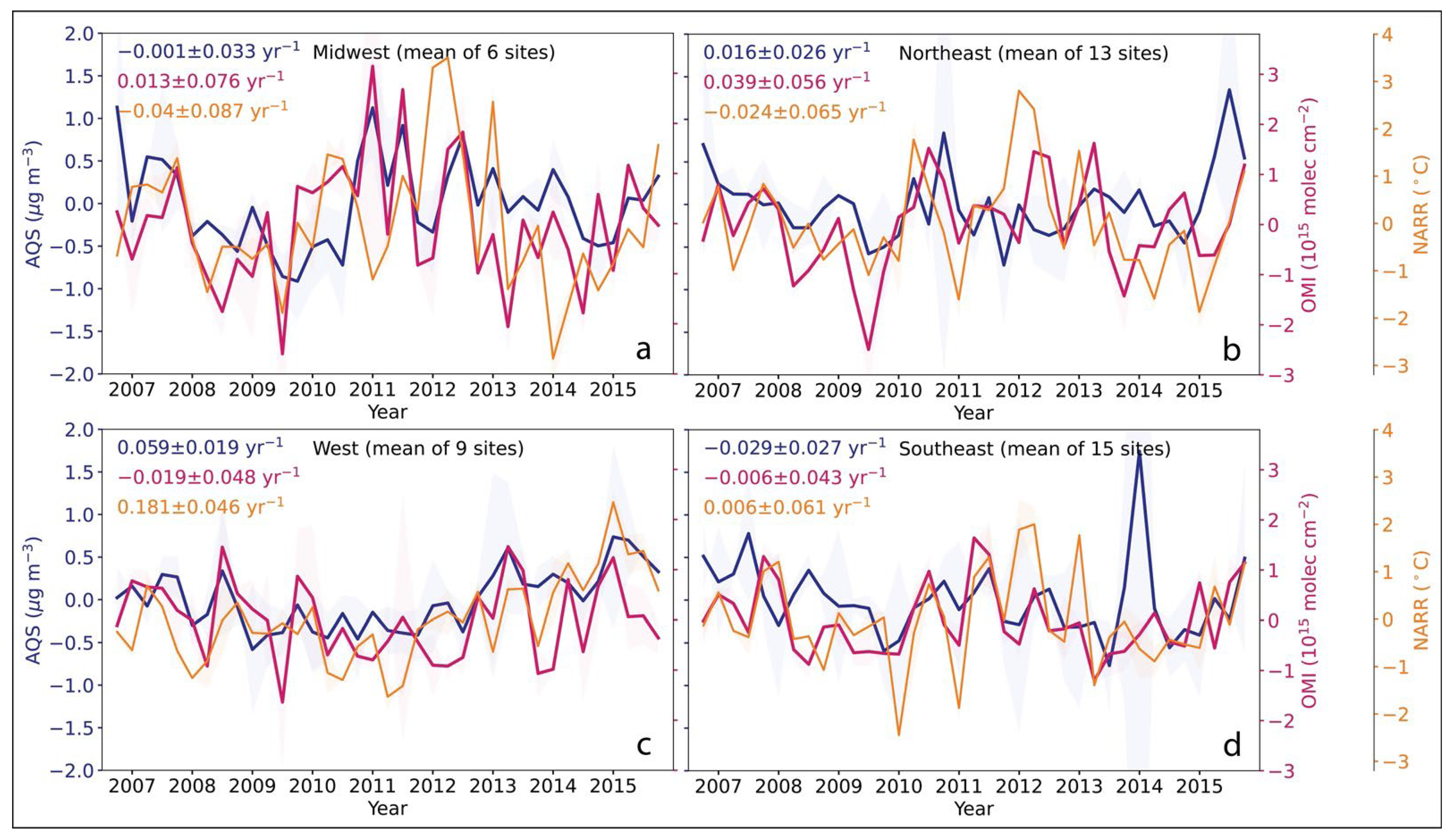
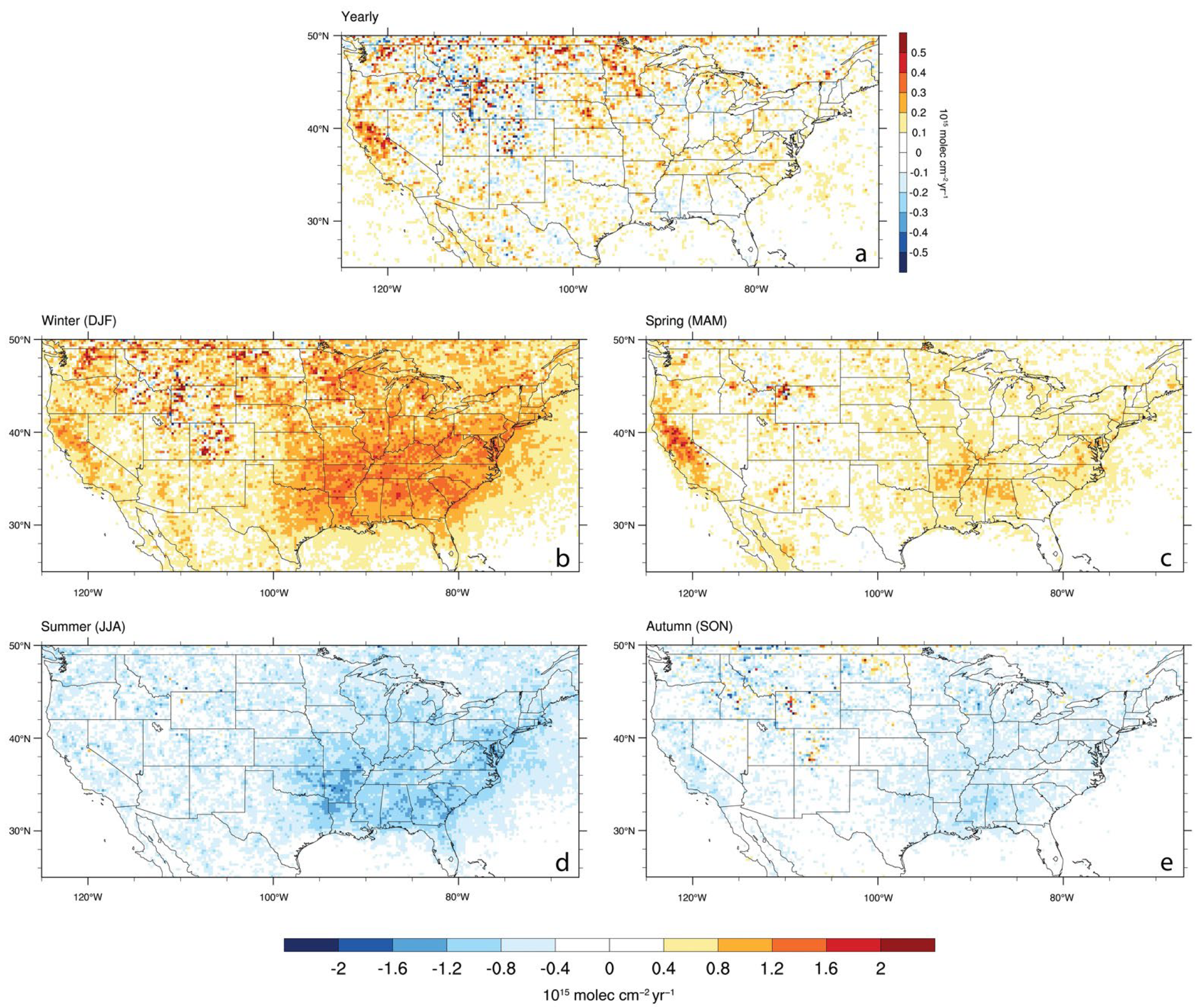
5. Interannual Trends

In Section 4.2, we showed that HCHO exhibits a strong seasonal cycle. To assess HCHO’s interannual variability between 2006 and 2015, we deseasonalized the seasonal mean values for each region, using observations from all 45 AQS stations and collocated OMI data. We also calculated the line of best fit for the deseasonalized data in each region. Endpoints are SON average 2006 and SON 2015 to avoid seasonality affecting the trend. Figure 5 shows the mean deseasonalized HCHO for AQS and OMI in each region (solid lines). These plots are overlaid with collocated seasonal average 2 m temperature from the North American Regional Reanalysis (NARR) [79], to indicate the role of temperature in the variability of each data set. The slopes from the linear regression and the associated standard errors are indicated in each panel.
After deseasonlizing the data, AQS and OMI show some consistency in certain periods. For example, both AQS and OMI captured the double peak in HCHO in 2010–2012 over the Midwest (Figure 5a). Both AQS and OMI HCHO also show elevated amounts in the west in summer of 2008 (Figure 5c), possibly corresponding to local fire emissions. However, the vertical and horizontal transport of VOC emissions from fires are more likely captured by satellite observations, and then affect regional trends downstream of fires more in the OMI record than in AQS.
During the entire ten-year period, the slopes from the linear regression on AQS and OMI do not aways agree. Since the standard errors associated with the slopes are rather large, this indicates HCHO did not have a significant and monotonic drift during 2006–2015. There are two exceptions: AQS in the west does indicate a significant increasing trend at a rate of 0.059 ± 0.019 μg m−3 yr−1, and AQS in the southeast is decreasing at a rate of 0.029 ± 0.027 μg m−3 yr−1 from 2006 to 2015. The large standard error in the southeast AQS data could partially come from the winter in 2014, when the regional mean is skewed by a few exceptionally high values.
In all regions, the increase in HCHO is partially explained by temperature trends, as shown by the NARR data. The west, which shows a significant increase in AQS HCHO, also shows the greatest warming at a rate of 0.181 ± 0.046 °C yr−1. However, this large increase is not captured by OMI, despite OMI having high agreement in seasonal variability with AQS. The interannual variations in temperature are also more quiescent in the western U.S. than in other regions, which could partially explain smaller year-to-year variations in HCHO in the West.
We used the same best fit linear regression to consider interannual changes for each season (Figure 6) and yearly mean for every grid box from OMI. We see a significant increase in California at around 0.3 × 10¹⁵ molec cm−2 per year; this is mostly contributed by an increase in MAM. The broader southeast and northeast regions experienced a strong increase in HCHO during DJF but were offset by a strong decrease in JJA. Such a decrease in HCHO could be partially explained by summertime cooling in the southeast U.S. over the past few decades [80,81].
Though OMI (co-located with AQS sites) indicates a decreasing trend that is opposite to AQS and NARR in the west (Figure 5c), there is a significant increase in OMI HCHO over large area of California, Oregon and Washington (Figure 6). Thus, using the OMI co-located pixels at AQS sites might not be indicative of the entire region.

6. Discussion

The evaluation of diurnal, seasonal, and interannual HCHO suggests that satellite-derived HCHO serves as a useful indicator for surface HCHO change on seasonal to interannual timescales. While surface-to-column agreement varies in space and time, the combined analysis of these two datasets informs the chemical and meteorological processes that impact HCHO.
This study builds on the earlier work of [72], with a greater focus on seasonality, temperature, and comparison between satellite and ground-based data. Whereas ref. [72] evaluated May-September change of temperature-corrected HCHO, we examine all seasons without removing temperature effects with the goal of characterizing the degree to which satellite data can inform near-surface trends and patterns.
The weighting function for OMI HCHO peaks in the upper troposphere [26], so it is well established that satellite data does not capture the same surface air as measured by the AQS monitors. With such differing physical characteristics between observation methods, it would be challenging to reconstruct ground level HCHO merely from satellite data. For example, ref. [82] reviewed methodologies of calculating surface level PM2.5 from satellite observed aerosol optical depth, which requires either a chemistry transport model or a statistical model based on empirical relations from the existing data. Future work to derive surface level HCHO from satellite observations could be made possible with such large datasets, such as the newly available EPA Air Quality Time Series (EQATES) project (available online, https://www.epa.gov/cmaq/equates; accessed on 21 April 2022).
Additionally, validation studies have shown that satellite HCHO tends to be biased low when column amounts are high (e.g., summer) and biased high when column amounts are low (e.g., winter), which would tend to dampen the OMI HCHO seasonal cycle [83,84,85]. Our observational results corroborate [35], who found that surface HCHO is a more significant contributor to column HCHO in the summer, based on model simulations. Despite the low agreement between AQS and OMI data in the winter, both datasets capture a consistent seasonal cycle and consistent interannual trends over certain periods.
Our findings suggest that temperature sensitivity of column HCHO is greater than near-surface HCHO. The seasonal amplitude of HCHO is higher in OMI data than in AQS in all regions, which may be due to the larger role of secondary HCHO in the column versus the surface. Furthermore, the warming across the 2006–2015 period leads to a stronger increase in the HCHO column in most regions, and a less-pronounced increase (or decrease) in the AQS monitor data, except in the west. The authors in [46] found that column NO2 is more sensitive to temperature than surface NO2, both in observations (monitors versus satellite) and in a numerical model; the same appears to be true for HCHO. As discussed by [72,86], trends in HCHO are attributable to a range of land use and emissions changes, independent of temperature. The impact of local emissions is evident in our results as well. In our analysis of diurnal HCHO at three sites with sufficient ground-data (Section 3), we found a mid-day peak in HCHO only at sites dominated by biogenic VOC emissions (Burbank and Pico Rivera in California). The increased temperature in the middle of the day accelerates the emission and oxidation of isoprene, consistent with [76]. Although current-generation satellites provide daily (or less frequent) HCHO data, the sensitivity of HCHO to temperature, including as a function of biogenic VOC emissions versus anthropogenic VOC emissions, would be a valuable application of future hourly HCHO observations from geostationary satellites.

7. Conclusions

As a pollutant with direct health impacts and an indicator of ozone formation, HCHO has emerged as an atmospheric species of interest for air quality management. Ground monitoring data of HCHO is limited, and satellite data may complement the sparse network with spatially continuous information on HCHO abundance. Multiple satellites can detect HCHO, but these data are only beginning to be applied to operational and health-relevant applications. For user communities interested in the interpretation of satellite data, a key question is the agreement in spatial and temporal patterns between ground-based and space-based measurements. Our comparison focuses on the utility of satellite data to inform patterns, trends, and processes of ground-based HCHO across the U.S.
Over our study period, HCHO data were available from 338 sites managed by the EPA. However, only 45 of these had continuous seasonal measurements in the time range, and only three stations provided hourly and three-hour measurement frequencies that had more than 10% data available and passed quality control. Of those three sites, the two sites with larger diurnal amplitudes (in Los Angeles County) had a lower anthropogenic/biogenic ratio for both direct HCHO emissions and for total VOC emissions, as compared to the site with the smaller diurnal amplitude (in St. Louis county). These relative diurnal changes indicate that the origin of VOC emissions may be an important driver of diurnal HCHO patterns. In addition to emissions, chemistry and meteorology also play important roles in affecting the diurnal cycle of HCHO. With the upcoming availability of hourly HCHO data from TEMPO, Sentinel-4, and GEMS, it will be interesting to assess how the diurnal amplitude of HCHO changes between areas dominated by biogenic versus anthropogenic emissions. We expect that areas with larger anthropogenic emissions will exhibit a weaker diurnal signal.
On a seasonal basis, OMI exhibits the highest correlation with AQS in summer and the lowest correlation in winter. These results are consistent with past work indicating that boundary layer HCHO is a greater contributor to the summertime HCHO column and less so in the winter [35]. Combining summer to other season ratios showed OMI bias is high compared to AQS in all regions, but with different factors depending on different regions. Seasonal differences across the regions are likely due to the differences in dominant plant types in each area, as well as VOC emissions in young versus mature trees [87]. The overestimation of the ratios from OMI suggests a more pronounced sensitivity to temperature in the HCHO column than in surface HCHO concentrations.
There are emerging opportunities to study HCHO and its trends in the near future from both ground- and space-based platforms. In 2021, U.S. states, in coordination with the EPA, established 27 new Photochemical Assessment Monitoring Stations (PAMS), which provide hourly ground-based HCHO measurements (official and supporting documents available at https://www.regulations.gov/document/EPA-HQ-OAR-2019-0137-0013; accessed on 22 April 2022). Additionally, ozone nonattainment areas have been required to develop Enhanced Monitoring Plans (EMP), which would expand observations of meteorology and VOCs, potentially including observations of columnar VOCs from PANDORA spectrometers [88]. In addition to these monitoring programs, next generation satellite-based observations are expected to provide high-resolution and hourly column HCHO measurements. Further analysis of space- versus ground-based measurements, using these next-generation platforms, will maximize the relevance of Earth-observing satellites to air quality and public health user communities.

Supplementary Materials

The following supporting information can be downloaded at: https://www.mdpi.com/article/10.3390/rs14092191/s1, Figure S1: All available AQS data from 2006 to 2015 calculated for every season (x-axis) compared with seasonal mean AQS under same OMI viewing conditions (y-axis), with correlation coefficient r = 0.999, mean bias = −0.005 µg m−3. Red dotted line indicates 1-1 ratio.

Author Contributions

Conceptualization, T.H.; Data curation, I.D.S.; Formal analysis, P.W. and M.B.; Funding acquisition, T.H.; Investigation, P.W.; Methodology, T.H.; Resources, M.H. and I.D.S.; Software, P.W.; Supervision, T.H.; Visualization, P.W. and M.B.; Writing—original draft, P.W. and M.H.; Writing—review & editing, T.H., M.B., M.H. and I.D.S. All authors have read and agreed to the published version of the manuscript.

Funding

This research and the APC were funded by the NASA Health and Air Quality Applied Sciences Team (HAQAST), grant numbers NNX16AQ92G and 80NSSC21K0427, as well as the Wisconsin Hilldale Undergraduate/Faculty Research Fellowship.

Data Availability Statement

Data and code for this study is available at https://doi.org/10.5281/zenodo.6499349 (accessed on 15 April 2022).

Acknowledgments

The authors acknowledge the processing of AQS data by Madeleine Strum from EPA. The authors appreciate the editorial contributions by Daegan Miller. Ground monitor data for HCHO is available at EPA AMA (https://www3.epa.gov/ttnamti1/toxdat.html#data; accessed on 30 August 2017), Satellite HCHO observations come from QA4ECV (available at http://www.qa4ecv.eu; accessed on 24 July 2019). EPA’s NEI data is available at https://www.epa.gov (accessed on 23 October 2017). NOAA North American Regional Reanalysis data is available at https://www.esrl.noaa.gov (accessed on 28 October 2016).

Conflicts of Interest

The authors declare no conflict of interest.

References

  1. Lowe, D.C.; Schmidt, U. Formaldehyde (HCHO) measurements in the nonurban atmosphere. J. Geophys. Res. 1983, 88, 10844. [Google Scholar] [CrossRef]
  2. Wolfe, G.M.; Kaiser, J.; Hanisco, T.F.; Keutsch, F.N.; de Gouw, J.A.; Gilman, J.B.; Graus, M.; Hatch, C.D.; Holloway, J.; Horowitz, L.W.; et al. Formaldehyde production from isoprene oxidation across NOx regimes. Atmos. Chem. Phys. 2016, 16, 2597–2610. [Google Scholar] [CrossRef] [PubMed] [Green Version]
  3. Sillman, S. Chapter 12 The relation between ozone, NOx and hydrocarbons in urban and polluted rural environments. Dev. Environ. Sci. 1998, 1, 339–385. [Google Scholar] [CrossRef]
  4. Palmer, P.I.; Jacob, D.J.; Fiore, A.M.; Martin, R.V.; Chance, K.; Kurosu, T.P. Mapping isoprene emissions over North America using formaldehyde column observations from space. J. Geophys. Res. Atmos. 2003, 108, 4180. [Google Scholar] [CrossRef] [Green Version]
  5. Millet, D.B.; Jacob, D.J.; Turquety, S.; Hudman, R.C.; Wu, S.; Fried, A.; Walega, J.; Heikes, B.G.; Blake, D.R.; Singh, H.B.; et al. Formaldehyde distribution over North America: Implications for satellite retrievals of formaldehyde columns and isoprene emission. J. Geophys. Res. Atmos. 2006, 111, D24S02. [Google Scholar] [CrossRef] [Green Version]
  6. Sprengnether, M.; Demerjian, K.L.; Donahue, N.M.; Anderson, J.G. Product analysis of the OH oxidation of isoprene and 1,3-butadiene in the presence of NO. J. Geophys. Res. Atmos. 2002, 107, ACH-8. [Google Scholar] [CrossRef]
  7. Levy, H. Photochemistry of the lower troposphere. Planet. Space Sci. 1972, 20, 919–935. [Google Scholar] [CrossRef]
  8. Atkinson, R. Atmospheric chemistry of VOCs and NOx. Atmos. Environ. 2000, 34, 2063–2101. [Google Scholar] [CrossRef]
  9. Abbot, D.S.; Palmer, P.I.; Martin, R.V.; Chance, K.V.; Jacob, D.J.; Guenther, A. Seasonal and interannual variability of North American isoprene emissions as determined by formaldehyde column measurements from space. Geophys. Res. Lett. 2003, 30, 1999–2002. [Google Scholar] [CrossRef] [Green Version]
  10. Holzinger, R.; Warneke, C.; Hansel, A.; Jordan, A.; Lindinger, W.; Scharffe, D.H.; Schade, G.; Crutzen, P.J. Biomass burning as a source of formaldehyde, acetaldehyde, methanol, acetone, acetonitrile, and hydrogen cyanide. Geophys. Res. Lett. 1999, 26, 1161–1164. [Google Scholar] [CrossRef]
  11. Piccot, S.D.; Watson, J.J.; Jones, J.W. A global inventory of volatile organic compound emissions from anthropogenic sources. J. Geophys. Res. Atmos. 1992, 97, 9897–9912. [Google Scholar] [CrossRef]
  12. Cárdenas, L.M.; Brassington, D.J.; Allan, B.J.; Coe, H.; Alicke, B.; Platt, U.; Wilson, K.M.; Plane, J.M.C.; Penkett, S.A. Intercomparison of Formaldehyde Measurements in Clean and Polluted Atmospheres. J. Atmos. Chem. 2000, 37, 53–80. [Google Scholar] [CrossRef]
  13. U.S. Environmental Protection Agency. Compendium Methods for the Determination of Toxic Organic Compounds in Ambient Air: Compendium Method TO-11A. 1999. Available online: https://www3.epa.gov/ttnamti1/files/ambient/airtox/to-11ar.pdf (accessed on 30 August 2017).
  14. Arnts, R.R.; Tejada, S.B. 2,4-Dinitrophenylhydrazine-coated silica gel cartridge method for determination of formaldehyde in air: Identification of an ozone interference. Environ. Sci. Technol. 1989, 23, 1428–1430. [Google Scholar] [CrossRef]
  15. Karst, U.; Binding, N.; Cammann, K.; Witting, U. Interferences of nitrogen dioxide in the determination of aldehydes and ketones by sampling on 2,4-dinitrophenylhydrazine-coated solid sorbent. Fresenius’ J. Anal. Chem. 1993, 345, 48–52. [Google Scholar] [CrossRef]
  16. Rodier, D.R.; Nondek, L.; Birks, J.W. Evaluation of ozone and water vapor interferences in the derivatization of atmospheric aldehydes with dansylhydrazine. Environ. Sci. Technol. 1993, 27, 2814–2820. [Google Scholar] [CrossRef]
  17. Achatz, S.; Lörinci, G.; Hertkorn, N.; Gebefügi, I.; Kettrup, A. Disturbance of the determination of aldehydes and ketones: Structural elucidation of degradation products derived from the reaction of 2,4-dinitrophenylhydrazine (DNPH) with ozone. Fresenius’ J. Anal. Chem. 1999, 364, 141–146. [Google Scholar] [CrossRef]
  18. Levelt, P.F.; Van Den Oord, G.H.J.; Dobber, M.R.; Malkki, A.; Visser, H.; De Vries, J.; Stammes, P.; Lundell, J.O.V.; Saari, H. The ozone monitoring instrument. IEEE Trans. Geosci. Remote. Sens. 2006, 44, 1093–1101. [Google Scholar] [CrossRef]
  19. Veefkind, J.P.; Aben, I.; McMullan, K.; Förster, H.; de Vries, J.; Otter, G.; Claas, J.; Eskes, H.J.; de Haan, J.F.; Kleipool, Q.; et al. TROPOMI on the ESA Sentinel-5 Precursor: A GMES mission for global observations of the atmospheric composition for climate, air quality and ozone layer applications. Remote Sens. Environ. 2012, 120, 70–83. [Google Scholar] [CrossRef]
  20. Abad, G.G.; Vasilkov, A.; Seftor, C.; Liu, X.; Chance, K. Smithsonian Astrophysical Observatory Ozone Mapping and Profiler Suite (SAO OMPS) formaldehyde retrieval. Atmos. Meas. Tech. 2016, 9, 2797–2812. [Google Scholar] [CrossRef] [Green Version]
  21. Munro, R.; Lang, R.; Klaes, D.; Poli, G.; Retscher, C.; Lindstrot, R.; Huckle, R.; Lacan, A.; Grzegorski, M.; Holdak, A.; et al. The GOME-2 instrument on the Metop series of satellites: Instrument design, calibration, and level 1 data processing—An overview. Atmos. Meas. Tech. 2016, 9, 1279–1301. [Google Scholar] [CrossRef] [Green Version]
  22. Kim, J.; Jeong, U.; Ahn, M.-H.; Kim, J.H.; Park, R.J.; Lee, H.; Song, C.H.; Choi, Y.-S.; Lee, K.-H.; Yoo, J.-M.; et al. New Era of Air Quality Monitoring from Space: Geostationary Environment Monitoring Spectrometer (GEMS). Bull. Am. Meteorol. Soc. 2020, 101, E1–E22. [Google Scholar] [CrossRef] [Green Version]
  23. Kwon, H.-A.; Park, R.J.; Abad, G.G.; Chance, K.; Kurosu, T.P.; Kim, J.; De Smedt, I.; Van Roozendael, M.; Peters, E.; Burrows, J. Description of a formaldehyde retrieval algorithm for the Geostationary Environment Monitoring Spectrometer (GEMS). Atmos. Meas. Tech. 2019, 12, 3551–3571. [Google Scholar] [CrossRef] [Green Version]
  24. Zoogman, P.; Liu, X.; Suleiman, R.; Pennington, W.; Flittner, D.; Al-Saadi, J.; Hilton, B.; Nicks, D.; Newchurch, M.; Carr, J.; et al. Tropospheric emissions: Monitoring of pollution (TEMPO). J. Quant. Spectrosc. Radiat. Transf. 2016, 186, 17–39. [Google Scholar] [CrossRef] [Green Version]
  25. Bauwens, M.; Stavrakou, T.; Müller, J.-F.; De Smedt, I.; Van Roozendael, M.; van der Werf, G.R.; Wiedinmyer, C.; Kaiser, J.W.; Sindelarova, K.; Guenther, A. Nine years of global hydrocarbon emissions based on source inversion of OMI formaldehyde observations. Atmos. Chem. Phys. 2016, 16, 10133–10158. [Google Scholar] [CrossRef] [Green Version]
  26. De Smedt, I.; Stavrakou, T.; Hendrick, F.; Danckaert, T.; Vlemmix, T.; Pinardi, G.; Theys, N.; Lerot, C.; Gielen, C.; Vigouroux, C.; et al. Diurnal, seasonal and long-term variations of global formaldehyde columns inferred from combined OMI and GOME-2 observations. Atmos. Chem. Phys. 2015, 15, 12519–12545. [Google Scholar] [CrossRef] [Green Version]
  27. Kaiser, J.; Wolfe, G.M.; Bohn, B.; Broch, S.; Fuchs, H.; Ganzeveld, L.N.; Gomm, S.; Häseler, R.; Hofzumahaus, A.; Holland, F.; et al. Evidence for an unidentified non-photochemical ground-level source of formaldehyde in the Po Valley with potential implications for ozone production. Atmos. Chem. Phys. 2015, 15, 1289–1298. [Google Scholar] [CrossRef] [Green Version]
  28. Kaiser, J.; Wolfe, G.M.; Min, K.E.; Brown, S.S.; Miller, C.C.; Jacob, D.J.; Degouw, J.A.; Graus, M.; Hanisco, T.F.; Holloway, J.; et al. Reassessing the ratio of glyoxal to formaldehyde as an indicator of hydrocarbon precursor speciation. Atmos. Chem. Phys. 2015, 15, 7571–7583. [Google Scholar] [CrossRef] [Green Version]
  29. Kefauver, S.C.; Filella, I.; Peñuelas, J. Remote sensing of atmospheric biogenic volatile organic compounds (BVOCs) via satellite-based formaldehyde vertical column assessments. Int. J. Remote Sens. 2014, 35, 7519–7542. [Google Scholar] [CrossRef]
  30. Kwon, H.-A.; Park, R.J.; Jeong, J.I.; Lee, S.; Abad, G.G.; Kurosu, T.P.; Palmer, P.I.; Chance, K. Sensitivity of formaldehyde (HCHO) column measurements from a geostationary satellite to temporal variation of the air mass factor in East Asia. Atmos. Chem. Phys. 2017, 17, 4673–4686. [Google Scholar] [CrossRef] [Green Version]
  31. Wells, K.C.; Millet, D.B.; Payne, V.H.; Deventer, M.J.; Bates, K.H.; de Gouw, J.A.; Graus, M.; Warneke, C.; Wisthaler, A.; Fuentes, J.D. Satellite isoprene retrievals constrain emissions and atmospheric oxidation. Nature 2020, 585, 225–233. [Google Scholar] [CrossRef]
  32. Wolfe, G.M.; Nicely, J.M.; Clair, J.M.S.; Hanisco, T.F.; Liao, J.; Oman, L.D.; Brune, W.B.; Miller, D.; Thames, A.; Abad, G.G.; et al. Mapping hydroxyl variability throughout the global remote troposphere via synthesis of airborne and satellite formaldehyde observations. Proc. Natl. Acad. Sci. USA 2019, 116, 11171–11180. [Google Scholar] [CrossRef] [PubMed] [Green Version]
  33. Zheng, Y.; Unger, N.; Barkley, M.P.; Yue, X. Relationships between photosynthesis and formaldehyde as a probe of isoprene emission. Atmos. Chem. Phys. 2015, 15, 8559–8576. [Google Scholar] [CrossRef] [Green Version]
  34. Harkey, M.; Holloway, T.; Kim, E.J.; Baker, K.R.; Henderson, B. Satellite Formaldehyde to Support Model Evaluation. J. Geophys. Res. Atmos. 2021, 126, e2020JD032881. [Google Scholar] [CrossRef]
  35. Jin, X.; Fiore, A.M.; Murray, L.T.; Valin, L.C.; Lamsal, L.N.; Duncan, B.; Boersma, K.F.; De Smedt, I.; Abad, G.G.; Chance, K.; et al. Evaluating a Space-Based Indicator of Surface Ozone-NOx-VOC Sensitivity Over Midlatitude Source Regions and Application to Decadal Trends. J. Geophys. Res. Atmos. 2017, 122, 10439–10461. [Google Scholar] [CrossRef] [PubMed]
  36. Jin, X.; Fiore, A.; Boersma, K.F.; De Smedt, I.; Valin, L. Inferring Changes in Summertime Surface Ozone–NOx–VOC Chemistry over U.S. Urban Areas from Two Decades of Satellite and Ground-Based Observations. Environ. Sci. Technol. 2020, 54, 6518–6529. [Google Scholar] [CrossRef] [PubMed]
  37. Li, D.; Wang, S.; Xue, R.; Zhu, J.; Zhang, S.; Sun, Z.; Zhou, B. OMI-observed HCHO in Shanghai, China, during 2010–2019 and ozone sensitivity inferred by an improved HCHO/NO2 ratio. Atmos. Chem. Phys. 2021, 21, 15447–15460. [Google Scholar] [CrossRef]
  38. Palmer, P.; Abbot, D.S.; Fu, T.-M.; Jacob, D.J.; Chance, K.; Kurosu, T.P.; Guenther, A.; Wiedinmyer, C.; Stanton, J.C.; Pilling, M.J.; et al. Quantifying the seasonal and interannual variability of North American isoprene emissions using satellite observations of the formaldehyde column. J. Geophys. Res. Atmos. 2006, 111, D12315. [Google Scholar] [CrossRef] [Green Version]
  39. Duncan, B.N.; Prados, A.; Lamsal, L.N.; Liu, Y.; Streets, D.G.; Gupta, P.; Hilsenrath, E.; Kahn, R.A.; Nielsen, J.E.; Beyersdorf, A.J.; et al. Satellite data of atmospheric pollution for U.S. air quality applications: Examples of applications, summary of data end-user resources, answers to FAQs, and common mistakes to avoid. Atmos. Environ. 2014, 94, 647–662. [Google Scholar] [CrossRef] [Green Version]
  40. Hong, Q.; Liu, C.; Hu, Q.; Zhang, Y.; Xing, C.; Su, W.; Ji, X.; Xiao, S. Evaluating the feasibility of formaldehyde derived from hyperspectral remote sensing as a proxy for volatile organic compounds. Atmos. Res. 2021, 264, 105777. [Google Scholar] [CrossRef]
  41. Martin, R.; Parrish, D.D.; Ryerson, T.B.; Nicks, D.K.; Chance, K.; Kurosu, T.P.; Jacob, D.J.; Sturges, E.D.; Fried, A.; Wert, B.P. Evaluation of GOME satellite measurements of tropospheric NO2 and HCHO using regional data from aircraft campaigns in the southeastern United States. J. Geophys. Res. Atmos. 2004, 109, D24307. [Google Scholar] [CrossRef]
  42. Duncan, B.N.; Yoshida, Y.; Olson, J.R.; Sillman, S.; Martin, R.; Lamsal, L.; Hu, Y.; Pickering, K.E.; Retscher, C.; Allen, D.; et al. Application of OMI observations to a space-based indicator of NOx and VOC controls on surface ozone formation. Atmos. Environ. 2010, 44, 2213–2223. [Google Scholar] [CrossRef] [Green Version]
  43. Witman, S.; Holloway, T.; Reddy, P.J. Integrating Satellite Data into Air Quality Management: Experience from Colorado; Air and Waste Management Association: Pittsburgh, PA, USA, 2014; pp. 34–38. [Google Scholar]
  44. Martin, R.V.; Jacob, D.J.; Chance, K.; Kurosu, T.P.; Palmer, P.; Evans, M.J. Global inventory of nitrogen oxide emissions constrained by space-based observations of NO2 columns. J. Geophys. Res. Atmos. 2003, 108, 4537. [Google Scholar] [CrossRef] [Green Version]
  45. Lamsal, L.N.; Martin, R.; Van Donkelaar, A.; Steinbacher, M.; Celarier, E.A.; Bucsela, E.; Dunlea, E.J.; Pinto, J.P. Ground-level nitrogen dioxide concentrations inferred from the satellite-borne Ozone Monitoring Instrument. J. Geophys. Res. Atmos. 2008, 113, D16308. [Google Scholar] [CrossRef] [Green Version]
  46. Harkey, M.; Holloway, T.; Oberman, J.; Scotty, E. An evaluation of CMAQ NO2 using observed chemistry-meteorology correlations. J. Geophys. Res. Atmos. 2015, 120, 11775–11797. [Google Scholar] [CrossRef]
  47. Kramer, L.; Leigh, R.J.; Remedios, J.J.; Monks, P.S. Comparison of OMI and ground-based in situ and MAX-DOAS measurements of tropospheric nitrogen dioxide in an urban area. J. Geophys. Res. Atmos. 2008, 113, D16S39. [Google Scholar] [CrossRef]
  48. Boersma, K.F.; Jacob, D.J.; Trainic, M.; Rudich, Y.; DeSmedt, I.; Dirksen, R.; Eskes, H.J. Validation of urban NO2 concentrations and their diurnal and seasonal variations observed from the SCIAMACHY and OMI sensors using in situ surface measurements in Israeli cities. Atmos. Chem. Phys. 2009, 9, 3867–3879. [Google Scholar] [CrossRef] [Green Version]
  49. Ma, J.Z.; Beirle, S.; Jin, J.L.; Shaiganfar, R.; Yan, P.; Wagner, T. Tropospheric NO2 vertical column densities over Beijing: Results of the first three years of ground-based MAX-DOAS measurements (2008–2011) and satellite validation. Atmos. Chem. Phys. 2013, 13, 1547–1567. [Google Scholar] [CrossRef] [Green Version]
  50. Opacka, B.; Müller, J.-F.; Stavrakou, T.; Bauwens, M.; Sindelarova, K.; Markova, J.; Guenther, A.B. Global and regional impacts of land cover changes on isoprene emissions derived from spaceborne data and the MEGAN model. Atmos. Chem. Phys. 2021, 21, 8413–8436. [Google Scholar] [CrossRef]
  51. Wang, H.; Wu, Q.; Guenther, A.B.; Yang, X.; Wang, L.; Xiao, T.; Li, J.; Feng, J.; Xu, Q.; Cheng, H. A long-term estimation of biogenic volatile organic compound (BVOC) emission in China from 2001–2016: The roles of land cover change and climate variability. Atmos. Chem. Phys. 2021, 21, 4825–4848. [Google Scholar] [CrossRef]
  52. Gopikrishnan, G.; Kuttippurath, J. A decade of satellite observations reveal significant increase in atmospheric formaldehyde from shipping in Indian Ocean. Atmos. Environ. 2020, 246, 118095. [Google Scholar] [CrossRef]
  53. Shen, L.; Jacob, D.J.; Zhu, L.; Zhang, Q.; Zheng, B.; Sulprizio, M.P.; Li, K.; De Smedt, I.; Abad, G.G.; Cao, H.; et al. The 2005–2016 Trends of Formaldehyde Columns Over China Observed by Satellites: Increasing Anthropogenic Emissions of Volatile Organic Compounds and Decreasing Agricultural Fire Emissions. Geophys. Res. Lett. 2019, 46, 4468–4475. [Google Scholar] [CrossRef] [Green Version]
  54. Bauwens, M.; Verreyken, B.; Stavrakou, T.; Müller, J.-F.; De Smedt, I. Spaceborne evidence for significant anthropogenic VOC trends in Asian cities over 2005–2019. Environ. Res. Lett. 2022, 17, 015008. [Google Scholar] [CrossRef]
  55. Guan, J.; Jin, B.; Ding, Y.; Wang, W.; Li, G.; Ciren, P. Global Surface HCHO Distribution Derived from Satellite Observations with Neural Networks Technique. Remote Sens. 2021, 13, 4055. [Google Scholar] [CrossRef]
  56. Millet, D.B.; Jacob, D.J.; Boersma, K.; Fu, T.-M.; Kurosu, T.P.; Chance, K.; Heald, C.L.; Guenther, A. Spatial distribution of isoprene emissions from North America derived from formaldehyde column measurements by the OMI satellite sensor. J. Geophys. Res. Atmos. 2008, 113, D16308. [Google Scholar] [CrossRef]
  57. Zhu, L.; Mickley, L.J.; Jacob, D.J.; Marais, E.A.; Sheng, J.; Hu, L.; Abad, G.G.; Chance, K. Long-term (2005–2014) trends in formaldehyde (HCHO) columns across North America as seen by the OMI satellite instrument: Evidence of changing emissions of volatile organic compounds. Geophys. Res. Lett. 2017, 44, 7079–7086. [Google Scholar] [CrossRef]
  58. Duncan, B.N.; Yoshida, Y.; Damon, M.R.; Douglass, A.R.; Witte, J.C. Temperature dependence of factors controlling isoprene emissions. Geophys. Res. Lett. 2009, 36, L05813. [Google Scholar] [CrossRef]
  59. Guenther, A.; Geron, C.; Pierce, T.; Lamb, B.; Harley, P.; Fall, R. Natural emissions of non-methane volatile organic compounds, carbon monoxide, and oxides of nitrogen from North America. Atmos. Environ. 2000, 34, 2205–2230. [Google Scholar] [CrossRef] [Green Version]
  60. Tingey, D.T.; Manning, M.; Grothaus, L.C.; Burns, W.F. The Influence of Light and Temperature on Isoprene Emission Rates from Live Oak. Physiol. Plant. 1979, 47, 112–118. [Google Scholar] [CrossRef]
  61. Zhu, L.; Jacob, D.J.; Mickley, L.J.; Marais, E.; Cohan, D.; Yoshida, Y.; Duncan, B.N.; Abad, G.G.; Chance, K. Anthropogenic emissions of highly reactive volatile organic compounds in eastern Texas inferred from oversampling of satellite (OMI) measurements of HCHO columns. Environ. Res. Lett. 2014, 9, 114004. [Google Scholar] [CrossRef] [Green Version]
  62. Lieschke, K.J.; Fisher, J.A.; Paton-Walsh, C.; Jones, N.B.; Greenslade, J.W.; Burden, S.; Griffith, D.W.T. Decreasing Trend in Formaldehyde Detected From 20-Year Record at Wollongong, Southeast Australia. Geophys. Res. Lett. 2019, 46, 8464–8473. [Google Scholar] [CrossRef] [Green Version]
  63. Morfopoulos, C.; Müller, J.; Stavrakou, T.; Bauwens, M.; De Smedt, I.; Friedlingstein, P.; Prentice, I.C.; Regnier, P. Vegetation responses to climate extremes recorded by remotely sensed atmospheric formaldehyde. Glob. Chang. Biol. 2021, 28, 1809–1822. [Google Scholar] [CrossRef] [PubMed]
  64. Lorente, A.; Boersma, K.F.; Yu, H.; Dörner, S.; Hilboll, A.; Richter, A.; Liu, M.; Lamsal, L.N.; Barkley, M.; De Smedt, I.; et al. Structural uncertainty in air mass factor calculation for NO2 and HCHO satellite retrievals. Atmos. Meas. Tech. 2017, 10, 759–782. [Google Scholar] [CrossRef] [Green Version]
  65. De Smedt, I.; Yu, H.; Richter, A.; Beirle, S.; Eskes, H.; Boersma, K.F.; Van Roozendael, J.; Van Geffen, A.; Lorente, E.; Peters, E. QA4ECV HCHO Tropospheric Column Data from OMI; (Version 1.1) [Data set]; Royal Belgian Institute for Space Aeronomy: Uccle, Belgium, 2017. [Google Scholar] [CrossRef]
  66. De Smedt, I.; Theys, N.; Yu, H.; Danckaert, T.; Lerot, C.; Compernolle, S.; Van Roozendael, M.; Richter, A.; Hilboll, A.; Peters, E.; et al. Algorithm theoretical baseline for formaldehyde retrievals from S5P TROPOMI and from the QA4ECV project. Atmos. Meas. Tech. 2018, 11, 2395–2426. [Google Scholar] [CrossRef] [Green Version]
  67. Zhu, L.; Jacob, D.J.; Kim, P.S.; Fisher, J.A.; Yu, K.; Travis, K.R.; Mickley, L.J.; Yantosca, R.M.; Sulprizio, M.P.; De Smedt, I.; et al. Observing atmospheric formaldehyde (HCHO) from space: Validation and intercomparison of six retrievals from four satellites (OMI, GOME2A, GOME2B, OMPS) with SEAC4RS aircraft observations over the southeast US. Atmos. Chem. Phys. 2016, 16, 13477–13490. [Google Scholar] [CrossRef] [Green Version]
  68. Franco, B.; Marais, E.A.; Bovy, B.; Bader, W.; Lejeune, B.; Roland, G.; Servais, C.; Mahieu, E. Diurnal cycle and multi-decadal trend of formaldehyde in the remote atmosphere near 46° N. Atmos. Chem. Phys. 2016, 16, 4171–4189. [Google Scholar] [CrossRef] [Green Version]
  69. Lamsal, L.N.; Duncan, B.N.; Yoshida, Y.; Krotkov, N.A.; Pickering, K.E.; Streets, D.G.; Lu, Z.U.S. NO2 trends (2005–2013): EPA Air Quality System (AQS) data versus improved observations from the Ozone Monitoring Instrument (OMI). Atmos. Environ. 2015, 110, 130–143. [Google Scholar] [CrossRef]
  70. Kim, J.H.; Kim, S.M.; Baek, K.H.; Wang, L.; Kurosu, T.; De Smedt, I.; Chance, K.; Newchurch, M.J. Evaluation of satellite-derived HCHO using statistical methods. Atmos. Chem. Phys. Discuss. 2011, 11, 8003–8025. [Google Scholar] [CrossRef]
  71. Marais, E.A.; Jacob, D.J.; Kurosu, T.P.; Chance, K.; Murphy, J.G.; Reeves, C.; Mills, G.; Casadio, S.; Millet, D.B.; Barkley, M.P.; et al. Isoprene emissions in Africa inferred from OMI observations of formaldehyde columns. Atmos. Chem. Phys. 2012, 12, 6219–6235. [Google Scholar] [CrossRef] [Green Version]
  72. Zhu, L.; Jacob, D.J.; Keutsch, F.N.; Mickley, L.J.; Scheffe, R.; Strum, M.; Abad, G.G.; Chance, K.; Yang, K.; Rappenglück, B.; et al. Formaldehyde (HCHO) As a Hazardous Air Pollutant: Mapping Surface Air Concentrations from Satellite and Inferring Cancer Risks in the United States. Environ. Sci. Technol. 2017, 51, 5650–5657. [Google Scholar] [CrossRef]
  73. Stavrakou, T.; Müller, J.-F.; De Smedt, I.; Van Roozendael, M.; van der Werf, G.R.; Giglio, L.; Guenther, A. Evaluating the performance of pyrogenic and biogenic emission inventories against one decade of space-based formaldehyde columns. Atmos. Chem. Phys. 2009, 9, 1037–1060. [Google Scholar] [CrossRef] [Green Version]
  74. Carlton, A.G.; Baker, K.R. Photochemical Modeling of the Ozark Isoprene Volcano: MEGAN, BEIS, and Their Impacts on Air Quality Predictions. Environ. Sci. Technol. 2011, 45, 4438–4445. [Google Scholar] [CrossRef] [PubMed]
  75. Fuentes, J.D.; Wang, D.; Neumann, H.H.; Gillespie, T.J.; Hartog, G.D.; Dann, T.F. Ambient biogenic hydrocarbons and isoprene emissions from a mixed deciduous forest. J. Atmos. Chem. 1996, 25, 67–95. [Google Scholar] [CrossRef]
  76. Choi, W.; Faloona, I.C.; Bouvier-Brown, N.C.; McKay, M.; Goldstein, A.H.; Mao, J.; Brune, W.H.; LaFranchi, B.W.; Cohen, R.C.; Wolfe, G.M.; et al. Observations of elevated formaldehyde over a forest canopy suggest missing sources from rapid oxidation of arboreal hydrocarbons. Atmos. Chem. Phys. 2010, 10, 8761–8781. [Google Scholar] [CrossRef] [Green Version]
  77. Lin, J.-T.; McElroy, M.B. Impacts of boundary layer mixing on pollutant vertical profiles in the lower troposphere: Implications to satellite remote sensing. Atmos. Environ. 2010, 44, 1726–1739. [Google Scholar] [CrossRef]
  78. Pusede, S.E.; Gentner, D.R.; Wooldridge, P.J.; Browne, E.C.; Rollins, A.W.; Min, K.-E.; Russell, A.R.; Thomas, J.; Zhang, L.; Brune, W.H.; et al. On the temperature dependence of organic reactivity, nitrogen oxides, ozone production, and the impact of emission controls in San Joaquin Valley, California. Atmos. Chem. Phys. 2014, 14, 3373–3395. [Google Scholar] [CrossRef] [Green Version]
  79. Mesinger, F.; DiMego, G.; Kalnay, E.; Mitchell, K.; Shafran, P.C.; Ebisuzaki, W.; Jović, D.; Woollen, J.; Rogers, E.; Berbery, E.H.; et al. North American Regional Reanalysis. Bull. Am. Meteorol. Soc. 2006, 87, 343–360. [Google Scholar] [CrossRef] [Green Version]
  80. Mascioli, N.R.; Previdi, M.; Fiore, A.; Ting, M. Timing and seasonality of the United States ‘warming hole’. Environ. Res. Lett. 2017, 12, 034008. [Google Scholar] [CrossRef] [Green Version]
  81. Partridge, T.F.; Winter, J.M.; Osterberg, E.C.; Hyndman, D.W.; Kendall, A.D.; Magilligan, F.J. Spatially Distinct Seasonal Patterns and Forcings of the U.S. Warming Hole. Geophys. Res. Lett. 2018, 45, 2055–2063. [Google Scholar] [CrossRef]
  82. Diao, M.; Holloway, T.; Choi, S.; O’Neill, S.M.; Al-Hamdan, M.Z.; Van Donkelaar, A.; Martin, R.V.; Jin, X.; Fiore, A.M.; Henze, D.K.; et al. Methods, availability, and applications of PM2.5 exposure estimates derived from ground measurements, satellite, and atmospheric models. J. Air Waste Manag. Assoc. 2019, 69, 1391–1414. [Google Scholar] [CrossRef]
  83. De Smedt, I.; Pinardi, G.; Vigouroux, C.; Compernolle, S.; Bais, A.; Benavent, N.; Boersma, F.; Chan, K.-L.; Donner, S.; Eichmann, K.-U.; et al. Comparative assessment of TROPOMI and OMI formaldehyde observations and validation against MAX-DOAS network column measurements. Atmos. Chem. Phys. 2021, 21, 12561–12593. [Google Scholar] [CrossRef]
  84. Vigouroux, C.; Langerock, B.; Aquino, C.A.B.; Blumenstock, T.; Cheng, Z.; De Mazière, M.; De Smedt, I.; Grutter, M.; Hannigan, J.W.; Jones, N.; et al. TROPOMI–Sentinel-5 Precursor formaldehyde validation using an extensive network of ground-based Fourier-transform infrared stations. Atmos. Meas. Tech. 2020, 13, 3751–3767. [Google Scholar] [CrossRef]
  85. Zhu, L.; Abad, G.G.; Nowlan, C.R.; Miller, C.C.; Chance, K.; Apel, E.C.; DiGangi, J.P.; Fried, A.; Hanisco, T.F.; Hornbrook, R.S.; et al. Validation of satellite formaldehyde (HCHO) retrievals using observations from 12 aircraft campaigns. Atmos. Chem. Phys. 2020, 20, 12329–12345. [Google Scholar] [CrossRef]
  86. Fan, J.; Ju, T.; Wang, Q.; Gao, H.; Huang, R.; Duan, J. Spatiotemporal variations and potential sources of tropospheric formaldehyde over eastern China based on OMI satellite data. Atmos. Pollut. Res. 2020, 12, 272–285. [Google Scholar] [CrossRef]
  87. Bracho-Nunez, A.; Welter, S.; Staudt, M.; Kesselmeier, J. Plant-specific volatile organic compound emission rates from young and mature leaves of Mediterranean vegetation. J. Geophys. Res. Atmos. 2011, 116, 1–13. [Google Scholar] [CrossRef]
  88. U.S. Environmental Protection Agency. Technical Note—Guidance for Developing Enhanced Monitoring Plans. 2018. Available online: https://www.epa.gov/sites/default/files/2019-11/documents/pams_emp_guidance.pdf (accessed on 21 April 2022).
Figure 1. 2006–2015 annual average HCHO vertical column density from OMI. Four U.S. regions are designated for analysis, with region name aside the map. Overall, for studying diurnal patterns, there are three sites: two in the Western U.S. and one in the Midwest. These stations are labeled as triangles. For seasonal and interannual studies, there are 45 AQS stations (10 in the west, 6 in the Midwest, 14 in the southeast and 15 in the northeast) that are labeled as circles. For more details on monitoring sites, please see Section 2.1 and Table 1.
Remotesensing 14 02191 g001
Figure 2. HCHO mixing ratios from ground-based AQS monitors at three sites ((a): Burbank, CA; (b): St. Louis, MO; (c): Pico Rivera, CA) from 2006 to 2010. Solid lines show June, August, September (JAS) average diurnal cycle with complete measurements (24 measurements per day for 1 h site or 8 measurements per day for 3 h site). The shaded area indicates standard deviation in that averaging year. Different years are labeled in different colors, indicated in the bottom right. OMI overpass time (13:30 local time) is labeled with a vertical dashed line at each site.
Remotesensing 14 02191 g002
Figure 3. Spatial correlation of 2007–2015 average HCHO from 45 AQS sites (x-axis) and coincident OMI pixels (y-axis). Each point represents a single site, with OMI and AQS values averaged over the season. Points are color coded to reflect their region, and spatial correlation coefficient r values in different regions are shown in the legend. Each panel represents average values for: (a) winter, (b) spring, (c) summer, and (d) autumn.
Remotesensing 14 02191 g003
Figure 4. Summer to all other season ratios from AQS and OMI for the Midwest (a), northeast (b), west (c), and southeast (d). Red lines indicate regional median, green triangles indicate regional mean, and cycles represent extreme values.
Remotesensing 14 02191 g004
Figure 5. 2006–2015 AQS and OMI HCHO deseasonalized interannual trends averaged by season in the (a) Midwest, (b) northeast, (c) west, and (d) southeast. Blue lines indicate AQS trends, red lines represent OMI trends, and yellow represents 2 m temperature from the North American Regional Reanalysis (NARR) data, sampled at the AQS monitor locations. Solid lines are the mean seasonal HCHO abundance or temperatures, and shaded areas are the standard deviation. Region name and number of stations in the region are labeled at the top of each figure, along with the slope of the line of best fit and the standard errors associated with the slopes.
Remotesensing 14 02191 g005
Figure 6. Map of the U.S. with 2006–2015 OMI HCHO trend in (a) all seasons, (b) winter, (c) spring, (d) summer, and (e) autumn.
Remotesensing 14 02191 g006
Table 1. Number of HCHO ground monitoring stations in the United States, with data distributed by the EPA AQS. Stations are grouped based on data availability, and by measurement frequency (hourly, 3 h, and 24 h). Data availability is calculated as the percentage of measurements available from 2006 to 2015 relative to the potential number of measurements during this period at the monitor’s reporting frequency. The three sites used for analysis of the diurnal HCHO cycle are marked in bold, which include the 1 h site with 30–40% data availability (St. Louis, MO, USA), and the two 3 h site with 10–20% data availability (Burbank, CA, USA; Pico Rivera, CA, USA). These three sites are marked as triangle in Figure 1.
Percent Available1 h Frequency3 h Frequency24 h Frequency
0–10%939230
10–20%0270
20–30%0018
30–40%103
40–50%001
Total stations1041322
Table 2. 2006–2010 and 2008 (NEI reported year) mean June, August, September (JAS) diurnal HCHO amplitudes at the three AQS sites in Figure 2. Aabs is the absolute amplitude, and Arel is the relative amplitude.
Aabs (µg m−3)Arel (%)
2006–201020082006–20102008
Burbank, CA5.948.0553.9238.65
Pico Rivera, CA4.705.1380.4791.62
St. Louis, MO2.741.7634.7029.86
Table 3. 2008 NEI total VOC and HCHO emissions at St. Louis and Los Angeles county, along with anthropogenic to biogenic emissions ratio.
Total VOC Emissions (Kilotons)HCHO Emissions (Tons)
St. LouisLos AngelesSt. LouisLos Angeles
Biogenic6.4870.68101.431213.80
Anthropogenic36.33111.75338.582733.73
Wild Fire04.760295.65
Anthro/Bio Ratio5.611.583.342.25
Publisher’s Note: MDPI stays neutral with regard to jurisdictional claims in published maps and institutional affiliations.

