A Multi-Sensor Interacted Vehicle-Tracking Algorithm with Time-Varying Observation Error

Abstract

Vehicle tracking in the field of intelligent transportation has received extensive attention in recent years. Multi-sensor-based vehicle tracking system is widely used in some critical environments. However, in the actual scenes, the observation error of each sensor is often different and time varying because of the environmental change and the channel difference. Therefore, in this paper, we propose a multi-sensor interacted vehicle-tracking algorithm with time-varying observation error (MI-TVOE). The algorithm establishes a jointed and time-varying observation error model for each sensor to indicate the variation of observation noise. Then, we develop a multi-sensor interacted vehicle-tracking algorithm which can predict the statistical information of a time-varying observation error and fuse the tracking result of each sensor to provide a global estimation. Simulation results show that the proposed MI-TVOE algorithm can significantly improve the tracking performance compared to the single-sensor-based tracking method, the traditional unscented Kalman filter (UKF), the apdative UKF method (AUKF) and the multi-error fused UKF method (MEF-UKF), which will be well applied to the complex tracking scenes and will reduce the computational complexity with time-varying observation error. The experiments in this paper also prove the superiority of the proposed MI-TVOE algorithm in complex environments.

1. Introduction

With the advancement of computer technology, research on vehicle tracking in the field of intelligent transportation has received extensive attention [1,2,3]. Global Position System (GPS) is the most basic technology for vehicle tracking. However, GPS suffers from signal attenuation in some critical environments, such as urban canyons or indoors. In addition, vision-based localization methods are also used for vehicle tracking; however, they have poor tracking accuracy in the varying illumination conditions or shadows. In order to improve the tracking performance in these scenarios, a multi-sensor-based vehicle tracking system has been widely used, since it can fuse different kinds of observation data from each sensor, which can improve the tracking performance effectively [4,5,6,7].

However, in the actual scenarios, due to environmental change and channel difference, various noises and disturbances make the system more complex and unstable. Meanwhile, since the observation errors of each sensor are often different and time-varying, it is difficult to obtain the fixed noise distribution. Therefore, the multi-sensor-based vehicle tracking system still has great challenges in complicated scenarios. A new method needs to be developed to improve the system robustness and tracking accuracy.

In this paper, we propose a multi-sensor interacted vehicle-tracking algorithm with time-varying observation error to solve the described shortcomings. The main contributions of this paper are summarized as follows:

(1)

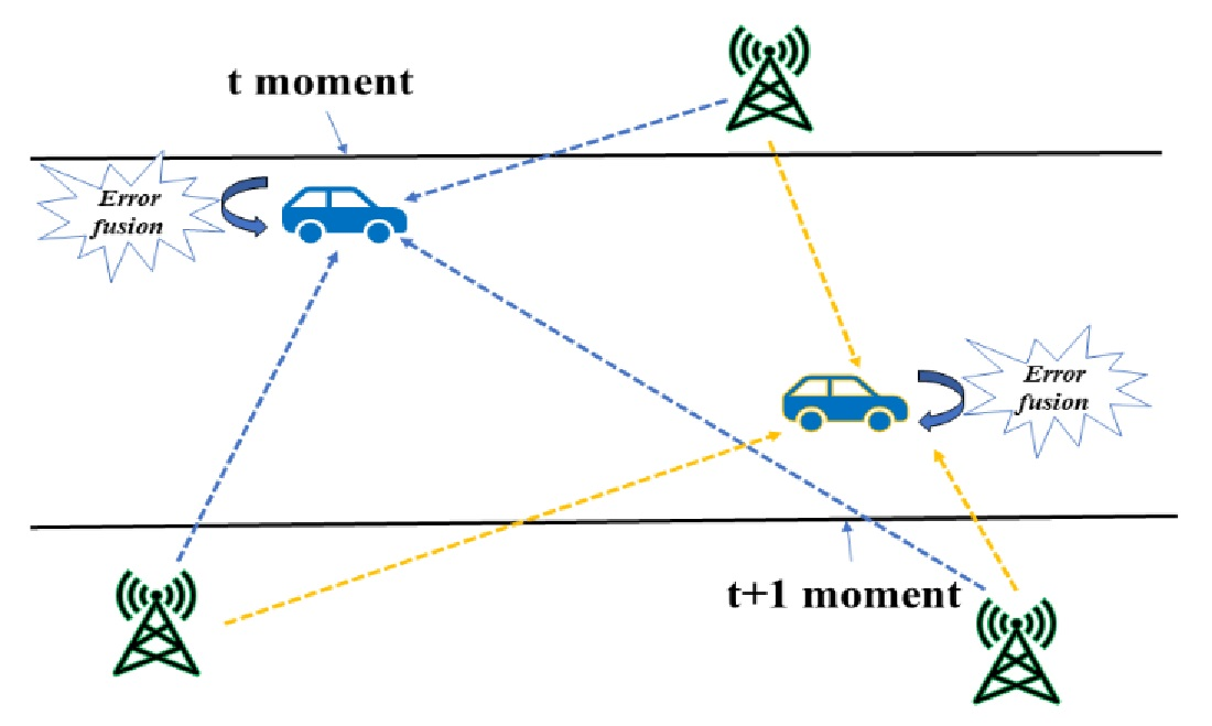
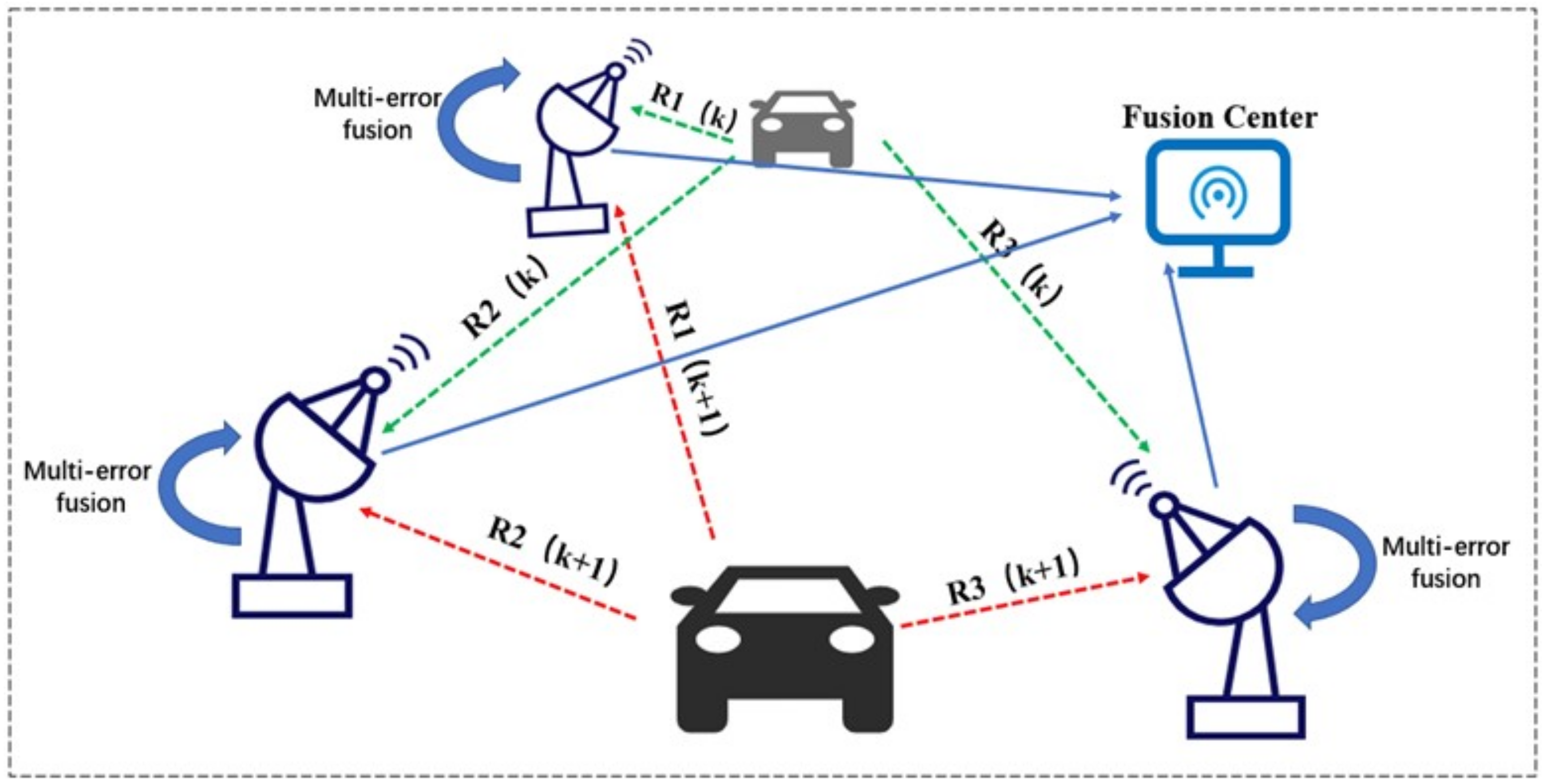
For complex tracking environments with changing noise, we establish a jointed and time-varying observation error model for each sensor to indicate the variation of observation noise, which improves the vehicle tracking performance with high tracking accuracy.

(2)

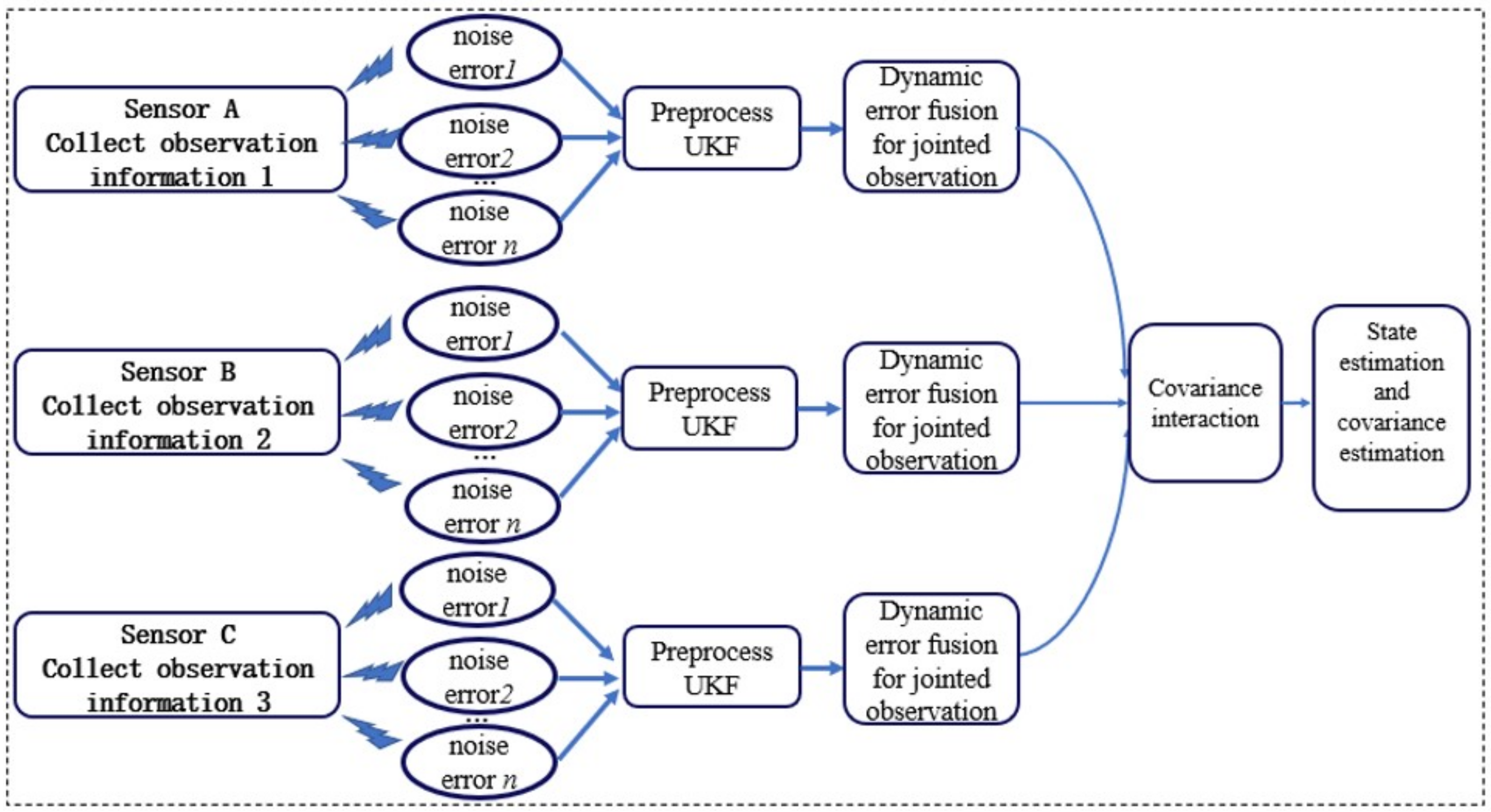
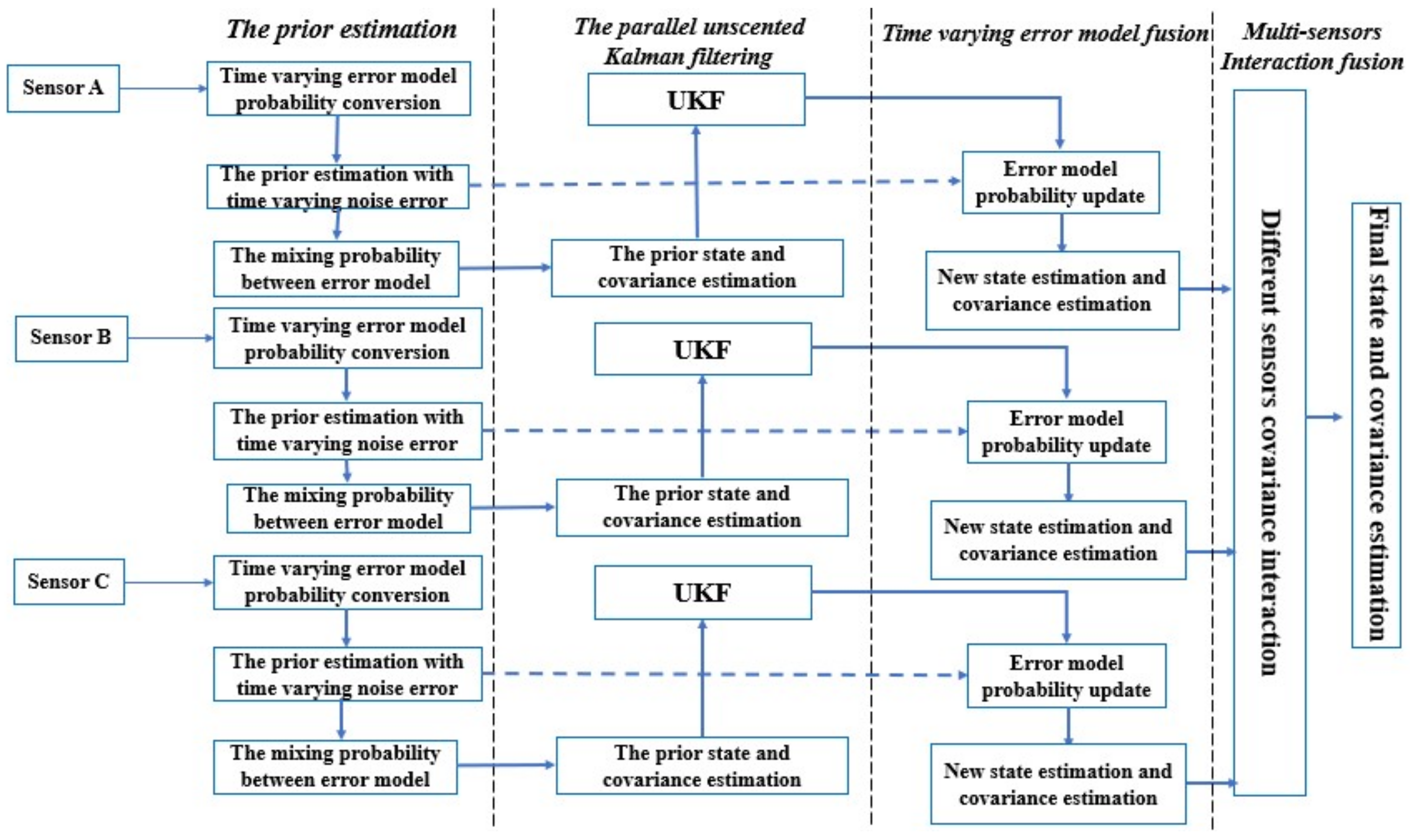
We propose a multi-sensor interacted vehicle-tracking algorithm which can predict the statistical information of time varying observation error and fuse the tracking result of each sensor to give a global estimation. The algorithm reduces the computational complexity and improve the tracking robustness with time varying observation error.

(3)

We verify the effectiveness of the proposed algorithm through simulation and experiments with real data. The experiments are performed by designing an unmanned mobile platform (UMP) positioning system with an inertial navigation system (INS) and ultra-wideband (UWB) platform. From the simulation and experiments result, we can improve the tracking performance significantly with time-varying observation noise.

This paper is organized as follows. Section 2 briefly reviews the related works about vehicle tracking. Section 3 introduces the system models, including the mobility model and the jointed observation model. In Section 4, we give the elaborate explanation of the new proposed MI-TVOE algorithm. The simulation process and analysis are introduced in Section 5. Section 6 gives the experiments results with real data to prove the effectiveness of the algorithm. Conclusions are drawn in Section 7.

Table 1. The MI-TVOE symbols.

Symbol	Definition
F	State transition matrix
$\mathbf{\Gamma }$	Input noise transition matrix
H	Observation matrix
w, v	System noise and measurement noise vector
Q, R	System and measurement covariance matrix
T	Sample period
$(x_p,y_p)$, $(x_v,y_v)$, $(x_a,y_a)$	The position, the velocity, and the acceleration of a moving vehicle
$(x_i,y_i)$	The position of sensor i
${Dist}_i$, ${Angle}_i$, ${Doppler}_i$	Distance, angle, and Doppler measurements of sensor i
${Rd}_{ij}$, ${Ra}_{ij}$, ${Rr}_{ij}$	The jth observation variance of sensor i for distance, angle, Doppler
$\mathbf{\Omega }$	Markov probability transition matrix
m	The number of different observation error models
N	The number of sensors
n	The dimension of the state vector
${\stackrel{-}{\mu }}_q$	The prediction probability of the q th observation error model
${\mu }_{jq}$	The mixing transition probability
${\stackrel{\wedge }{\mathbf{x}}}_{oq}$, ${\mathbf{P}}_{oq}$	The prior state vector and covariance estimation
${\stackrel{\wedge }{\mathbf{x}}}_j$, ${\mathbf{P}}_j$	The prediction state vector and covariance estimation
${{\mathbf{x}}_a}^{\left(j\right)}$, ${\omega }^{\left(j\right)}$	A series of sigma points and corresponding weight
${\stackrel{\wedge }{\mathbf{x}}}_q$, ${\mathbf{P}}_q$	One-step prediction of the sigma points
$\mathbf{z}$	Measurement (system output) vector
${\stackrel{\wedge }{\mathbf{x}}}_q$, ${\mathbf{P}}_q$	State vector and covariance matrix for one filter update
K	Gain of Unscented Kalman Filter
${\stackrel{\wedge }{\mathbf{x}}}_i$, ${\mathbf{P}}_i$	The estimation with time-varying observation error of sensor i
tr	Trace of the matrix
diag	Diagonal of vector or matrix
${}^{-1}$	Matrix inverse
${\omega }^i$	The fusion coefficient
${\stackrel{\wedge }{\mathbf{x}}}_g$, ${\mathbf{P}}_g$	The estimated results of the sensors fusion

provides a list of symbols used throughout the paper.

2. Related Works

2.1. Adaptive Tracking Methods

Bayesian filters are most commonly applied to vehicle tracking, including the Kalman filter (KF) [8], extended Kalman filter (EKF), unscented Kalman filter, and particle filter (PF) methods. Considering the complicated mobility and observation systems, many researchers have investigated the adaptive filter-based tracking algorithms. In [9], an online estimation method of adaptively distributing information coefficients is designed to solve the problem of low fusion tracking error and instability. For maneuvering vehicles, adaptive extended Kalman filter (AEKF) algorithms have been developed in [10,11] that can update the noise covariance during the estimation process. Ref. [12] proposed a random sample consensus(RANSAC)-based track initialization algorithm for a multi-sensor system, which could recursively learn the vehicle motion model in a noise environment. Considering the nonlinear observation systems, Ref. [13] proposed an adaptive tracking fusion algorithm based on UKF, which improved the distributed multi-sensor data fusion system and improved the tracking accuracy of ground combat vehicles. For the filtering problem of nonlinear systems, the filtering precision of UKF is higher than EKF, and the computation complexity of UKF is less than that of PF (Particle filter) [14,15]. Ref. [16] proposed a hierarchical fusion estimation method with link failures, which used the Kalman filter algorithm to ensure the consistency of the collected data and used a CI (Covariance Interaction) algorithm to obtain a fusion estimation, which dramatically reduced the computational complexity. In addition, Multiple Model (MM) and Interactive Multiple Model (IMM) algorithms [17,18] are widely used for the problem of unknown motion models in the maneuvering vehicle-tracking problem. Ref. [19] solved the problem of inability to assign precise regions for target vehicles and radar errors by using an IMM filter, improving the accuracy of measurements. However, the IMM algorithm also has some shortcomings, such as a large amount of calculation and a fixed model set.

2.2. Tracking Methods with Complex Noise

Although previous research has improved the tracking accuracy and reduced the computational complexity, the complex observation noise significantly impacts the tracking accuracy of the system as the time and environment change. It is of greater importance to study wireless channels with varying noise in complex scenarios. To deal with adaptive estimation of the noise covariance, Refs. [20,21] studied the state estimation problem of complex dynamic networks with nonlinear coupling under channel noise. Ref. [22] designed a new optimal estimation method for linear discrete time-systems with time-delay and multi-error measurement. This method improved the estimation accuracy by reducing the usage rate of measurement values with larger errors. When the target vehicles are affected by the tracking environment noise that is uncertain or completely unknown during the moving process, parameter estimation methods such as Recursive Least Squares (RLS) and the gradient algorithm have obtained great results. However, most of these estimation methods assume that the parameters to be estimated are constant or slowly changing. Subsequently, researchers considered the perspective of probability density function approximation, resulting in the Monte Carlo (MC) method [23], Variational Bayes (VB) [24,25] and Expectation Maximization (EM) [26] algorithm. Among them, variational Bayesian inference has become a tool for studying probabilistic models. It is more accurate and faster than traditional point estimation, and has higher filtering accuracy. Ref. [27] proposed an interactive multi-model variational Bayesian (IMM-VB) algorithm to solve the problem of tracking accuracy degradation caused by outlier interference in real systems. Ref. [28] proposed an adaptive extended vehicle-tracking algorithm with unknown time-varying sensor error covariance. In [29], an approximate maximization method based on variational inference is used for multi-camera 3D localization and video tracking, which is significantly better than previous algorithms. However, the variational Bayesian algorithm is computationally expensive in the continuous iterative process.

2.3. Real-Time Tracking Methods

For the actual vehicle-tracking scenarios, the observation noise is always varied with different time. Real-time processing performance is an essential aspect when the subject of vehicle tracking is addressed. Refs. [30,31,32,33] proposed real-time tracking maneuvering target algorithms. Ref. [30] develops a visual monitoring system and yield a stable, real-time tracker that reliably deals with the long-term scene changes. According to the needs of real-time tracking maneuvering targets, researchers combine the Gaussian algorithm and wavelet filtering to remove the influence of interference and obtain the target maneuvering trajectory in [31]. Meanwhile, in [33], an ultra-wideband and inertial navigation data fusion positioning algorithm based on Kalman filter (INS+KF) is proposed to deal with the problem of real-time tracking. Although these methods turned out to improve location accuracy based on simulation results, the robustness of these algorithms is poor when the environment changes suddenly.

2.4. Former Works

Our former work in [34] proposed an unscented Kalman-filter-based fusion tracking method with a multi-error model (MEF-UKF). In [34], we developed a multi-error model to describe the observation noise’s variation. Then, we obtained the tracking trajectory by fusing the results from several parallel unscented Kalman filters corresponding to each observation noise. However, the multi-error model in [34] can be only used with single observation, which has limited tracking performance. Meanwhile, if the sensor fails or no signal is received, it will cause great difficulties in tracking. Therefore, in this paper, we propose a jointed and time-varying observation error model which can indicate the changing measurement noise and develop a multi-sensor interacted method to obviously improve the tracking accuracy.

3. Models

In this paper, we construct a multi-sensor interacted vehicle-tracking system. The system structure used in intelligent transportation is as shown in Figure 1. In Figure 1, multiple sensors are deployed in the monitoring area, which can receive the observation information from the moving vehicles. The fusion center is used to obtain the global tracking result.

Affected by the environmental change and the channel difference, the observation noise error from each sensor is always different and time varying, which obviously reduces the tracking accuracy. In Figure 1, $\left\{R_1\left(k\right),R_2\left(k\right),R_3\left(k\right)\right\}$ and $\left\{R_1(k+1),R_2(k+1),R_3(k+1)\right\}$ determine the noise error vector of each sensor at time k and time $k+1$, respectively.

According to the system structure as shown in Figure 1, we introduce the vehicle-tracking system model from two parts: the mobility model and the jointed observation model.

3.1. Mobility Model

Consider a multi-sensor based vehicle tracking system. The mobility model is expressed as in (1),

$$\mathbf{x}(k+1)=\mathbf{F}\mathbf{x}\left(k\right)+\mathbf{\Gamma }\mathbf{w}\left(k\right)$$

(1)

$$\mathbf{x}\left(k\right)={\left[x_p\left(k\right) y_p\left(k\right) x_v\left(k\right) y_v\left(k\right) x_a\left(k\right) y_a\left(k\right)\right]}^T$$

(2)

$$\mathbf{F}=\left[\begin{array}{cccccc}1& 0& T& 0& \frac{T^2}{2}& 0\\ 0& 1& 0& T& 0& \frac{T^2}{2}\\ 0& 0& 1& 0& T& 0\\ 0& 0& 0& 1& 0& T\\ 0& 0& 0& 0& 1& 0\\ 0& 0& 0& 0& 0& 1\end{array}\right]$$

(3)

$$\mathbf{\Gamma }=\left[\begin{array}{cc}\frac{T^2}{4}& 0\\ 0& \frac{T^2}{4}\\ \frac{T}{2}& 0\\ 0& \frac{T}{2}\\ 1& 0\\ 0& 1\end{array}\right]$$

(4)

where $\mathbf{x}\left(k\right)$ is the state vector of a moving vehicle at time k. $(x_p\left(k\right),y_p\left(k\right))$, $(x_v\left(k\right),y_v\left(k\right))$ and $(x_a\left(k\right),y_a\left(k\right))$ represent the position, the velocity and the acceleration of a moving vehicle at time k, respectively. $\mathbf{F}$ is the state transition matrix. $\mathbf{\Gamma }$ is the input noise transition matrix, which can be obtained from (3) and (4). $\mathbf{w}\left(k\right)\sim N(0,\mathbf{Q}\left(k\right))$ is the model noise. $\mathbf{Q}\left(k\right)$ is the covariance matrix of $\mathbf{w}\left(k\right)$ at time k. T is the observation period.

3.2. Jointed Observation Model

The observation model describes the relationship between the observation $\mathbf{z}\left(k\right)$ and the system state $\mathbf{x}\left(k\right)$. Therefore, the observation model of the moving target can be expressed as (5),

$$\mathbf{z}\left(k\right)=\mathbf{H}\left(\mathbf{x}\right(k\left)\right)+\mathbf{v}\left(k\right)$$

(5)

where $\mathbf{H}$ represents the observation matrix of the system. $\mathbf{v}\left(k\right)\sim N(0,\mathbf{R}(k\left)\right)$ is the observation noise. ${\mathbf{R}}_k$ is the covariance of the observation noise at time k. Since the observation noise always varies with time and environment changes, $\mathbf{R}\left(k\right)$ is a time-varying parameter which will greatly affect the tracking performance. In this paper, we will analyze the time-varying noise error $\mathbf{R}\left(k\right)$ in detail in Section 3.

In order to increase the tracking precision, we use a jointed observation, including distance ${Dist}_i$, angle ${Angle}_i$ and Doppler measurements ${Doppler}_i$ of sensor i to describe the observation information from different aspects, which are as shown in (6)–(8).

$${Dist}_i=\sqrt{{(x_p\left(k\right)-x_i)}^2+{(y_p\left(k\right)-y_i)}^2}$$

(6)

$${Angle}_i=atan(y_p\left(k\right)-y_i)/(x_p\left(k\right)-x_i)$$

(7)

$${Doppler}_i=(x_v\left(k\right)\ast x_p\left(k\right)+y_v\left(k\right)\ast y_p\left(k\right))/\sqrt{{(x_p\left(k\right)-x_i)}^2+{(y_p\left(k\right)-y_i)}^2})$$

(8)

where $(x_i,y_i)$ represents the position of sensor i. $(x_p\left(k\right),y_p\left(k\right))$ is the moving vehicle’s position at time k. $(x_v\left(k\right),y_v\left(k\right))$ is the vehicle’s velocity at time k.

Based on the jointed observation information, we establish a jointed observation matrix as in (9).

$$\mathbf{H}=\left[\begin{array}{c}\sqrt{{(x_p\left(k\right)-x_i)}^2+{(y_p\left(k\right)-y_i)}^2}\\ atan(y_p\left(k\right)-y_i)/(x_p\left(k\right)-x_i)\\ (x_v\left(k\right)\ast x_p\left(k\right)+y_v\left(k\right)\ast y_p\left(k\right))/\sqrt{{(x_p\left(k\right)-x_i)}^2+{(y_p\left(k\right)-y_i)}^2})\end{array}\right]$$

(9)

4. Vehicle-Tracking Algorithm

In this paper, we propose a multi-sensor interacted vehicle-tracking algorithm with time-varying observation error. Firstly, we propose a time-varying and jointed observation error model to indicate the changing measurement noise. Then, a multi-sensor interacted vehicle-tracking algorithm is proposed to predict the statistical information of time-varying observation error and give a global tracking result by fusing the time-varying observation information from different sensors. Figure 2 is the block diagram of the proposed algorithm.

4.1. Jointed and Time Varying Observation Error Model

According to the prior analysis of each sensor’s observation in the monitoring area, we define a jointed variance matrix by combining some typical variance values for each sensor. The jth variance for sensor i at time k is as shown in (10),

$${\mathbf{R}}_{ij}\left(k\right)=\left[\begin{array}{ccc}{Rd}_{ij}\left(k\right)& 0& 0\\ 0& {Ra}_{ij}\left(k\right)& 0\\ 0& 0& {Rr}_{ij}\left(k\right)\end{array}\right]$$

(10)

where ${Rd}_{ij}\left(k\right)$, ${Ra}_{ij}\left(k\right)$ and ${Rr}_{ij}\left(k\right)$ are the observation variance for distance, angle, and Doppler measurements, respectively, at time k.

Since the observation error is constantly changing with time, on the basis of the jointed variance matrix, we establish a jointed and time varying observation error model to describe the dynamic observation error.

According to the jointed variance matrix, we assume that there are m different observation error models with different variances. Then the Markov probability transition matrix $\mathbf{\Omega }$ can be used to calculate the transition probability of different observation error models at different times.

$$\mathbf{\Omega }=\left[\begin{array}{ccc}{\mathbf{\Omega }}_{11}& \dots & {\mathbf{\Omega }}_{1m}\\ ⋮& \ddots & ⋮\\ {\mathbf{\Omega }}_{m1}& \cdots & {\mathbf{\Omega }}_{mm}\end{array}\right]$$

(11)

where ${\mathbf{\Omega }}_{jq}$ is the probability that the observation error model j transfers to the observation error model q.

The prediction probability of the qth observation error model ${\stackrel{-}{\mu }}_q (k+1|k)$ can be obtained from (12),

$${\stackrel{-}{\mu }}_q (k+1|k)=\sum _{j=1}^m{\mathbf{\Omega }}_{jq}{\mu }_j\left(k\right)$$

(12)

where ${\mu }_j\left(k\right)$ is the probability of the observation error model j at time k. ${\mu }_j\left(0\right)$ represents the initial probability of each observation error. ${\mathbf{\Omega }}_{jq}$ is the probability that the observation error model j transfers to the observation error model q.

The mixing transition probability from the qth observation error model to the jth observation error model ${\mu }_{jq}\left(k\right)$ is as in (13).

$${\mu }_{jq}\left(k\right)=\frac{{\mathbf{\Omega }}_{jq}{\mu }_j\left(k\right)}{{\stackrel{-}{\mu }}_q (k+1|k)}$$

(13)

We can use the mixing transition probability ${\mu }_{jq}\left(k\right)$ and the jointed variance matrix in (10) to describe the time varying observation error.

4.2. Multi-Sensor Interacted Vehicle Tracking Algorithm

Since the observation information from multiple sensors is uncorrelated and time varying, it is difficult to calculate the changing cross-covariance of each sensor and the precision of the vehicle-tracking system is low. In this paper, we develop a multi-sensor interacted vehicle-tracking algorithm by using a series of parallel UKF and interacting the uncorrelated covariance of each sensor with the proposed observation error model. The algorithm can predict the statistical information of time-varying observation error and provide a global tracking result with high precision.

4.2.1. The Prior Estimation

The prior state vector ${\stackrel{\wedge }{\mathbf{x}}}_{oq} \left(k\right)$ and the prior covariance estimation ${\mathbf{P}}_{oq}\left(k\right)$ are denoted as in (14) and (15), respectively, which can be used as the initial value for the parallel unscented Kalman filters. q denotes the qth observation error model.

$${\stackrel{\wedge }{\mathbf{x}}}_{oq} \left(k\right)=\sum _{j=1}^m{\stackrel{\wedge }{\mathbf{x}}}_j \left(k\right){\mu }_{jq}\left(k\right)$$

(14)

$${\mathbf{P}}_{oq}\left(k\right)=\sum _{j=1}^m{\mu }_{jq}\left(k\right)\{{\mathbf{P}}_j\left(k\right)+[{\stackrel{\wedge }{\mathbf{x}}}_j \left(k\right)-{\stackrel{\wedge }{\mathbf{x}}}_{oq} \left(k\right)]{[{\stackrel{\wedge }{\mathbf{x}}}_j \left(k\right)-{\stackrel{\wedge }{\mathbf{x}}}_{oq} \left(k\right)]}^T\}$$

(15)

where ${\stackrel{\wedge }{\mathbf{x}}}_j \left(k\right)$ and ${\mathbf{P}}_j\left(k\right)$ are the prediction results of the state vector and the covariance matrix, respectively, for observation error model j. m is the total number of the observation error models in the system. ${\mu }_{jq}\left(k\right)$ is the mixing transition probability from observation error model j to error model q, which is as shown in (13).

4.2.2. The Parallel Unscented Kalman Filters

We can update the state vector ${\stackrel{\wedge }{\mathbf{x}}}_j \left(k\right)$ and the covariance matrix ${\mathbf{P}}_j\left(k\right)$ of one kind of observation error model by using the unscented Kalman filter, as shown below.

Firstly, we can obtain a series of sigma points ${{\mathbf{x}}_a}^{\left(j\right)}\left(k\right)$ and their corresponding weights ${\omega }^{\left(j\right)}$ by using unscented transformation (UT) [35]. Then, the one-step prediction for $2n+1$ sigma points is as in (16)–(18):

$${{\mathbf{x}}_a}^{\left(j\right)}(k+1|k)=\mathbf{F}[{{\mathbf{x}}_a}^{\left(j\right)}\left(k\right)],j=1,2,\dots ,2n+1$$

(16)

$${\stackrel{\wedge }{\mathbf{x}}}_q (k+1|k)=\sum _{j=0}^{2n}{\omega }^{\left(j\right)}{{\mathbf{x}}_a}^{\left(j\right)}(k+1|k)$$

(17)

$${\mathbf{P}}_q(k+1|k)=\sum _{j=0}^{2n}\{{\omega }^{\left(j\right)}[{\stackrel{\wedge }{\mathbf{x}}}_q (k+1|k)-{{\mathbf{x}}_a}^{\left(j\right)}(k+1|k)]\times {[{\stackrel{\wedge }{\mathbf{x}} }_q(k+1|k)-{{\mathbf{x}}_a}^{\left(j\right)}(k+1|k)]}^T\}+\mathbf{Q}\left(k\right)$$

(18)

where ${\stackrel{\wedge }{\mathbf{x}}}_q (k+1|k)$, ${\mathbf{P}}_q(k+1|k)$ is the one-step prediction of the sigma points, the state vector and the covariance matrix, respectively. $\mathbf{F}$ is the state transition matrix as in (3). $\mathbf{Q}\left(k\right)$ is the covariance matrix of the mobility model.

Substituting the predicted sigma point ${{\mathbf{x}}_a}^{\left(j\right)}(k+1|k)$ into the observation Equation (5), the observation prediction is as shown in (19)–(22).

$${\mathbf{z}}^{\left(j\right)}(k+1|k)=\mathbf{H}[{{\mathbf{x}}_a}^{\left(j\right)}(k+1|k)]$$

(19)

$$\stackrel{-}{\mathbf{z}} (k+1|k)=\sum _{j=0}^{2n}{\omega }^{\left(j\right)}{\mathbf{z}}^{\left(j\right)}(k+1|k)$$

(20)

$${\mathbf{P}}_{z_k{z}_k}=\sum _{j=0}^{2n}\{{\omega }^{\left(j\right)}[{\mathbf{z}}^{\left(j\right)}(k+1|k)-\stackrel{-}{\mathbf{z}} (k+1|k)]\times {[{\mathbf{z}}^{\left(j\right)}(k+1|k)-\stackrel{-}{\mathbf{z}} (k+1|k)]}^T\}+{\mathbf{R}}_{ijk}$$

(21)

$${\mathbf{P}}_{x_k{z}_k}=\sum _{j=0}^{2n}\{{\omega }^{\left(j\right)}[{{\mathbf{x}}_a}^{\left(j\right)}(k+1|k)-\stackrel{-}{\mathbf{z}} (k+1|k)]\times {[{\mathbf{z}}^{\left(j\right)}(k+1|k)-\stackrel{-}{\mathbf{z}} (k+1|k)]}^T\}$$

(22)

According to (14)–(22), we can obtain the update value of state vector ${\stackrel{\wedge }{\mathbf{x}}}_q (k+1)$ and covariance matrix ${\mathbf{P}}_q(k+1)$ when the observation error model is turning from model j to model q.

$${\stackrel{\wedge }{\mathbf{x}}}_q (k+1)={\stackrel{\wedge }{\mathbf{x}}}_q (k+1|k)+\mathbf{K}(k+1)[\mathbf{z}(k+1)-\stackrel{-}{\mathbf{z}} (k+1|k)]$$

(23)

$${\mathbf{P}}_q(k+1)={\mathbf{P}}_q(k+1|k)-\mathbf{K}(k+1){\mathbf{P}}_{z_K{z}_K}{\mathbf{K}}^T(k+1)$$

(24)

$$\mathbf{K}(k+1)={\mathbf{P}}_{x_k{z}_k}{\mathbf{P}}_{z_k{z}_k}^{-1}$$

(25)

4.2.3. Vehicle Tracking with Time-Varying Observation Error

For time-varying observation noise, we can use the proposed observation error model to update the vehicle’s position precisely. Assume that there are m typical observation error models during the tracking process. The typical observation error models’ settings are based on the statistic analysis of the prior observations for the monitoring area. Then, the probabilistic fusion is performed according to (26)–(28) to obtain the estimation results of the state vector and the covariance matrix with time-varying observation noise.

The probability of observation error model q at time $k+1$ can be updated according to (26):

$${\mu }_q(k+1)=\frac{{\stackrel{-}{\mu }}_q (k+1|k)}{{\displaystyle \sum _{q=1}^m}{\stackrel{-}{\mu }}_q (k+1|k)}$$

(26)

where ${\stackrel{-}{\mu }}_q (k+1|k)$ is as shown in (12)

Then, the state estimation ${\stackrel{\wedge }{\mathbf{x}}}_i (k+1)$ and the covariance estimation ${\mathbf{P}}_i(k+1)$ with time-varying observation error for sensor i at time $k+1$ are as in (27) and (28).

$${\stackrel{\wedge }{\mathbf{x}}}_i (k+1)=\sum _{q=1}^m{\stackrel{\wedge }{\mathbf{x}}}_q (k+1){\mu }_q(k+1)$$

(27)

$${\mathbf{P}}_i(k+1)=\sum _{q=1}^m{\mu }_q(k+1)\{{\mathbf{P}}_q(k+1)+[{\stackrel{\wedge }{\mathbf{x}}}_q (k+1)-{\stackrel{\wedge }{\mathbf{x}}}_i (k+1)]\times {[{\stackrel{\wedge }{\mathbf{x}}}_q (k+1)-{\stackrel{\wedge }{\mathbf{x}}}_i (k+1)]}^T\}$$

(28)

where ${\stackrel{\wedge }{\mathbf{x}}}_q (k+1)$, ${\mathbf{P}}_q(k+1)$ are as shown in (23) and (24).

4.2.4. Vehicle Tracking with Multi-Sensor Interaction

Since the observation information from multiple sensors is uncorrelated and time varying, it is difficult to calculate the cross-covariance of the target tracking system. In this paper, we develop a covariance-interaction-based parallel UKF method with a time-varying observation error to deal with the target tracking problem for a multi-sensor system with unknown and changing covariance. The method only uses the local estimations of the state vector and the covariance matrix to obtain the tracking result for a multi-sensor system which ensures the consistency of the fusion results and greatly reduces the computational complexity.

For a vehicle-tracking system with N sensors, the global estimations of state vector ${\stackrel{\wedge }{\mathbf{x}}}_g (k+1)$ and covariance matrix ${\mathbf{P}}_g(k+1)$ are calculated by interacting each sensor’s result, which is as shown in (29) and (30).

$${\stackrel{\wedge }{\mathbf{x}}}_g (k+1)=\sum _{i=1}^N{\omega }_i{\mathbf{P}}_g{{\mathbf{P}}_i}^{-1}(k+1){\stackrel{\wedge }{\mathbf{x}}}_i (k+1)$$

(29)

$${{\mathbf{P}}_g}^{-1}(k+1)=\sum _{i=1}^N{\omega }_i{\mathbf{P}}_i^{-1}(k+1)$$

(30)

where ${\omega }_i$ is the fusion coefficient, which is obtained from (31) and (32), ${\stackrel{\wedge }{\mathbf{x}}}_i (k+1)$ is the state estimation of sensor i, and ${\mathbf{P}}_i(k+1)$ is the covariance estimation of sensor i.

$${\omega }_i=1/tr\left({\mathbf{P}}_g\right)=1/tr[\sum _{i=1}^N{\omega }_i{\mathbf{P}}_i^{-1}(k+1)]$$

(31)

$$\sum _{i=1}^N{\omega }_i=1$$

(32)

The flow diagram of the entire algorithm is as shown in Figure 3.

5. Simulation Results

In this part, we will give the simulation results of the proposed vehicle-tracking algorithm from different aspects in order to analyze the performance of the proposed algorithm.

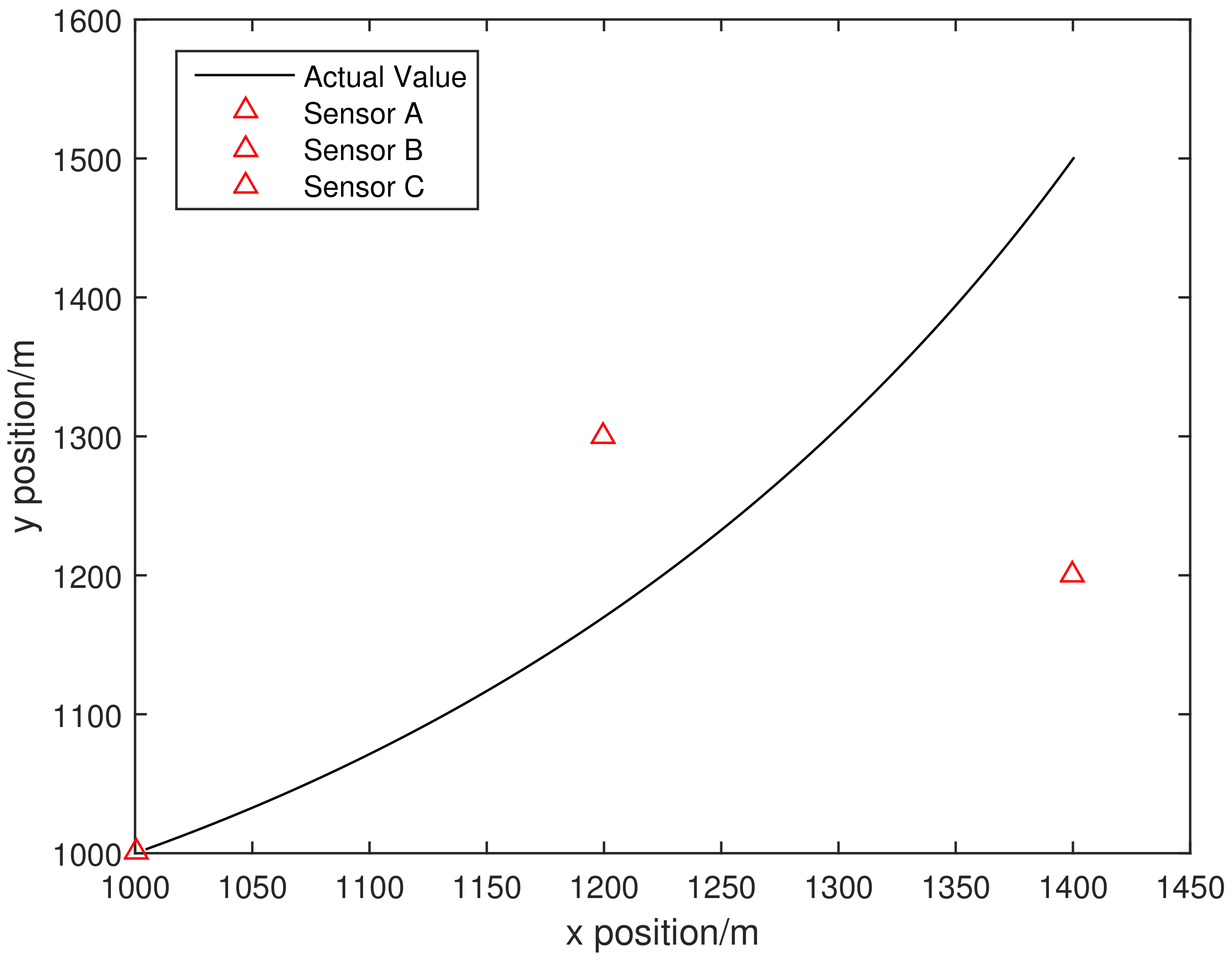
5.1. Simulation Environment Settings

Consider that the target is moving uniformly in a two-dimensional plane. The initial state vector of the target is $\mathbf{x}\left(0\right)=[1000 \mathrm{m};1000 \mathrm{m};50 \mathrm{m}/\mathrm{s};30 \mathrm{m}/\mathrm{s};-2 {\mathrm{m}/\mathrm{s}}^2;4 {\mathrm{m}/\mathrm{s}}^2]$. The prior state covariance matrix is given by ${\mathbf{P}}_0=\mathrm{diag}\left([0.1,0.1,0.1,0.1,0.1,0.1]\right)$. The total time is 100 s and the sampling period is 0.1 s. The number of sensors in the system is $N=3$ and the position of each sensor is shown in

Table 2. Some parameter settings of the simulation environment.

Parameter	Sensor A	Sensor B	Sensor C
Location	(1000 m, 1000 m)	(1200 m, 1300 m)	(1400 m, 1200 m)
Time-varying error model1 (distance, angle, Doppler noise)	$d_{11}=2^2$ $a_{11}={\left(\frac{0.1}{57.3}\right)}^2$ $r_{11}=1^2$	$d_{21}={1.3}^2$ $a_{21}={\left(\frac{0.15}{57.3}\right)}^2$ $r_{21}=1.5^2$	$d_{31}={1.4}^2$ $a_{31}={\left(\frac{0.1}{57.3}\right)}^2$ $r_{31}=1.8^2$
Time-varying error model2 (distance, angle, Doppler noise)	$d_{12}=1^2$ $a_{12}={\left(\frac{0.2}{57.3}\right)}^2$ $r_{12}={1.8}^2$	$d_{22}={1.2}^2$ $a_{22}={\left(\frac{0.2}{57.3}\right)}^2$ $r_{22}={2.2}^2$	$d_{32}=2^2$ $a_{32}={\left(\frac{0.18}{57.3}\right)}^2$ $r_{32}={2.5}^2$
Time-varying error model3 (distance, angle, Doppler noise)	$d_{13}=5^2$ $a_{13}={\left(\frac{0.3}{57.3}\right)}^2$ $r_{13}=2^2$	$d_{23}=3^2$ $a_{23}={\left(\frac{0.35}{57.3}\right)}^2$ $r_{23}={2.5}^2$	$d_{33}=3^2$ $a_{33}={\left(\frac{0.35}{57.3}\right)}^2$ $r_{33}=3^2$
Single-error model (distance, angle, Doppler noise)	$d_1=2^2$ $a_1={\left(\frac{0.1}{57.3}\right)}^2$ $r_1=1^2$	$d_2=1^2$ $a_2={\left(\frac{0.15}{57.3}\right)}^2$ $r_2={1.5}^2$	$d_3={1.5}^2$ $a_3={\left(\frac{0.1}{57.3}\right)}^2$ $r_3={1.8}^2$
Process noise	$\mathbf{Q}=\mathrm{diag}\left(\right[1,0.5,1,0.5,1,0.5\left]\right)$

. The total number of observation error models observed by each sensor is $m=3$. The following experimental results are all obtained with 100 Monte Carlo tests. The process noise Q and the observation noise R are shown in Table 2.

In this section, we use three sensors to track the mobile vehicle. These sensors can be used to send and receive observation information such as distance, angle, Doppler, etc. Meanwhile, they can also measure the distance between each other. Both simulation and experimental data are performed in a noisy environment.

Figure 4 shows the actual trajectory of the moving vehicle and the location of the three sensors.

5.2. Simulation Results Analysis

In this section, we will analyze the performance of the proposed MI-TVOE algorithm from different aspects. The comparison results are measured by using the tracking trajectory and the tracking Root Mean Square Error (RMSE).

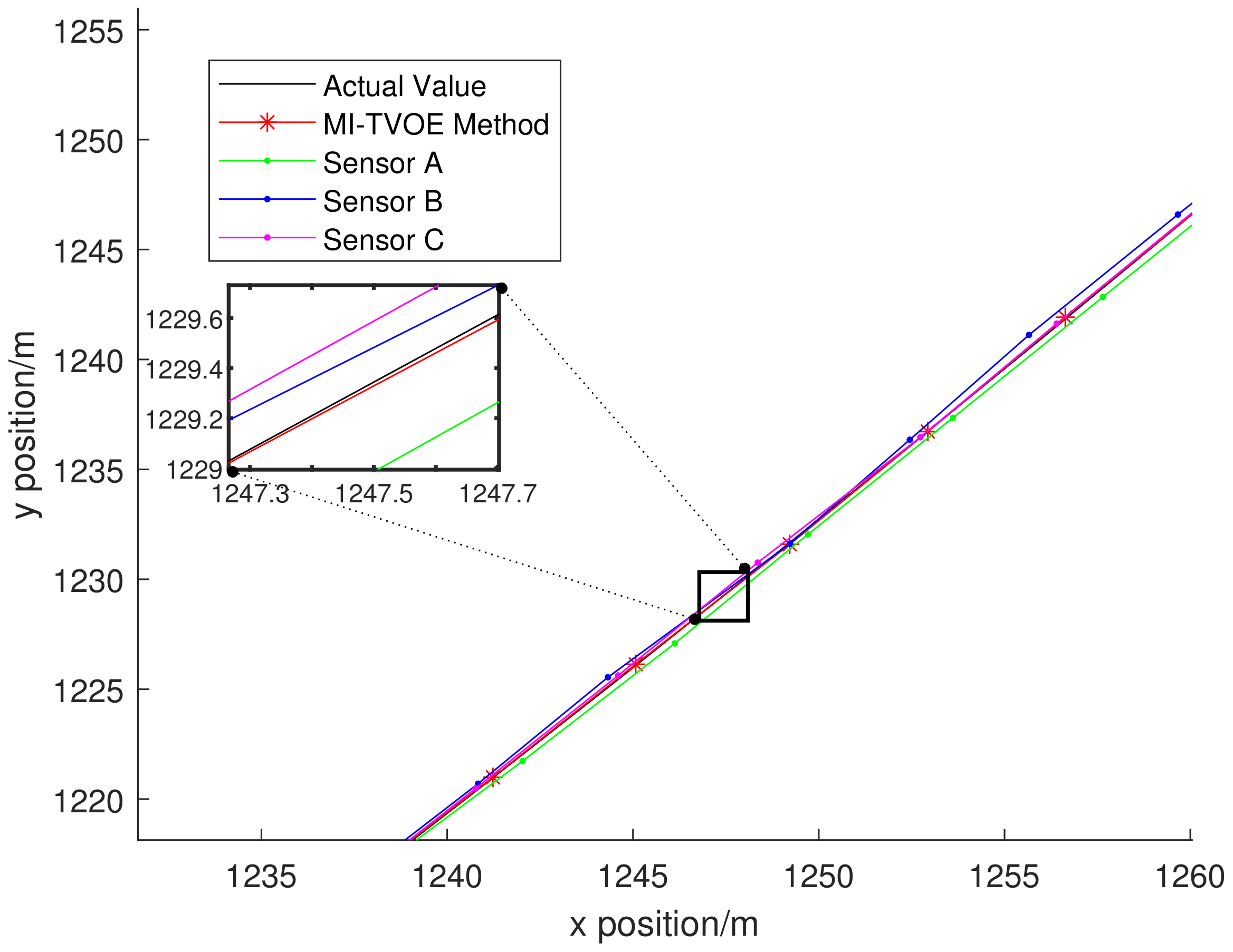
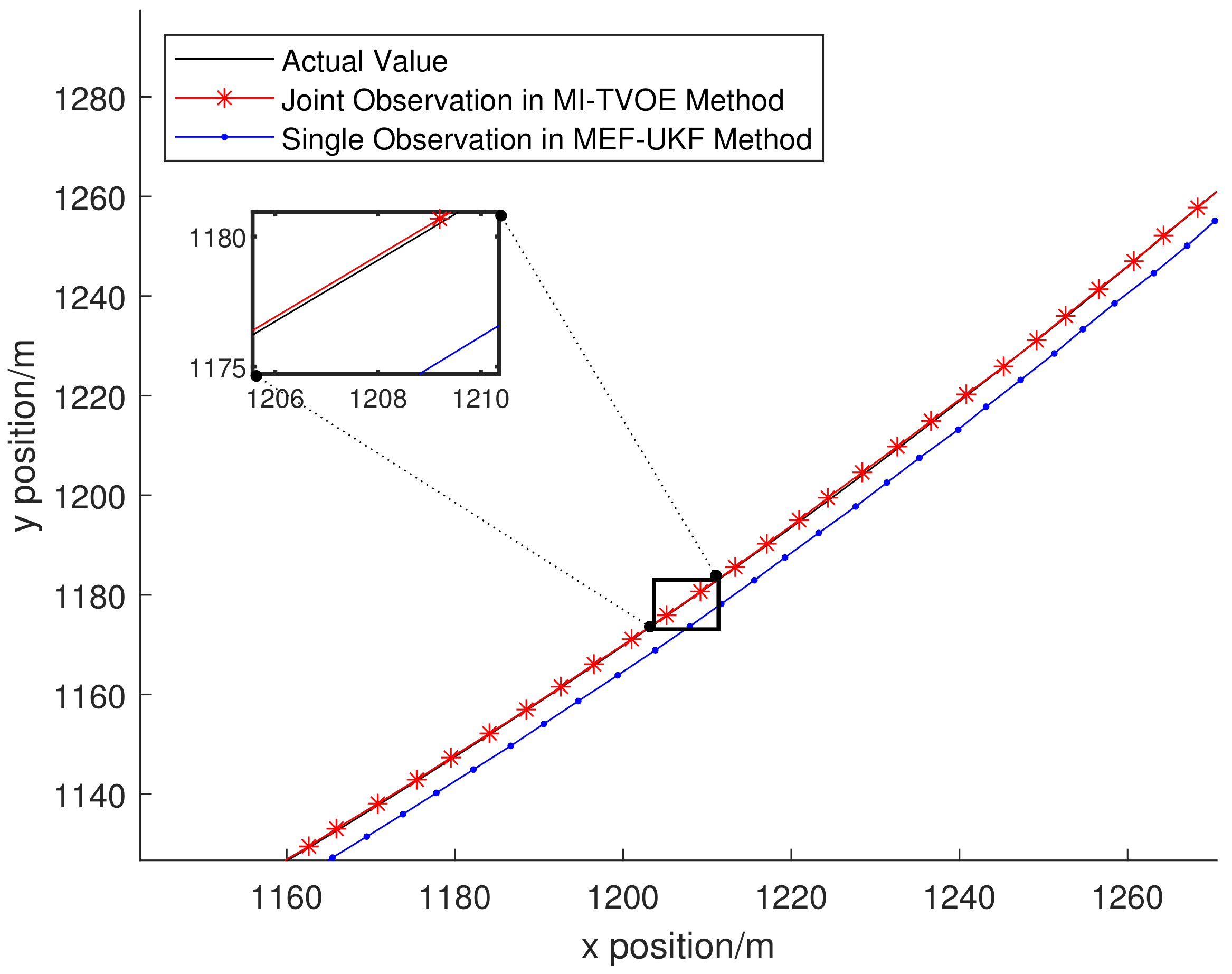
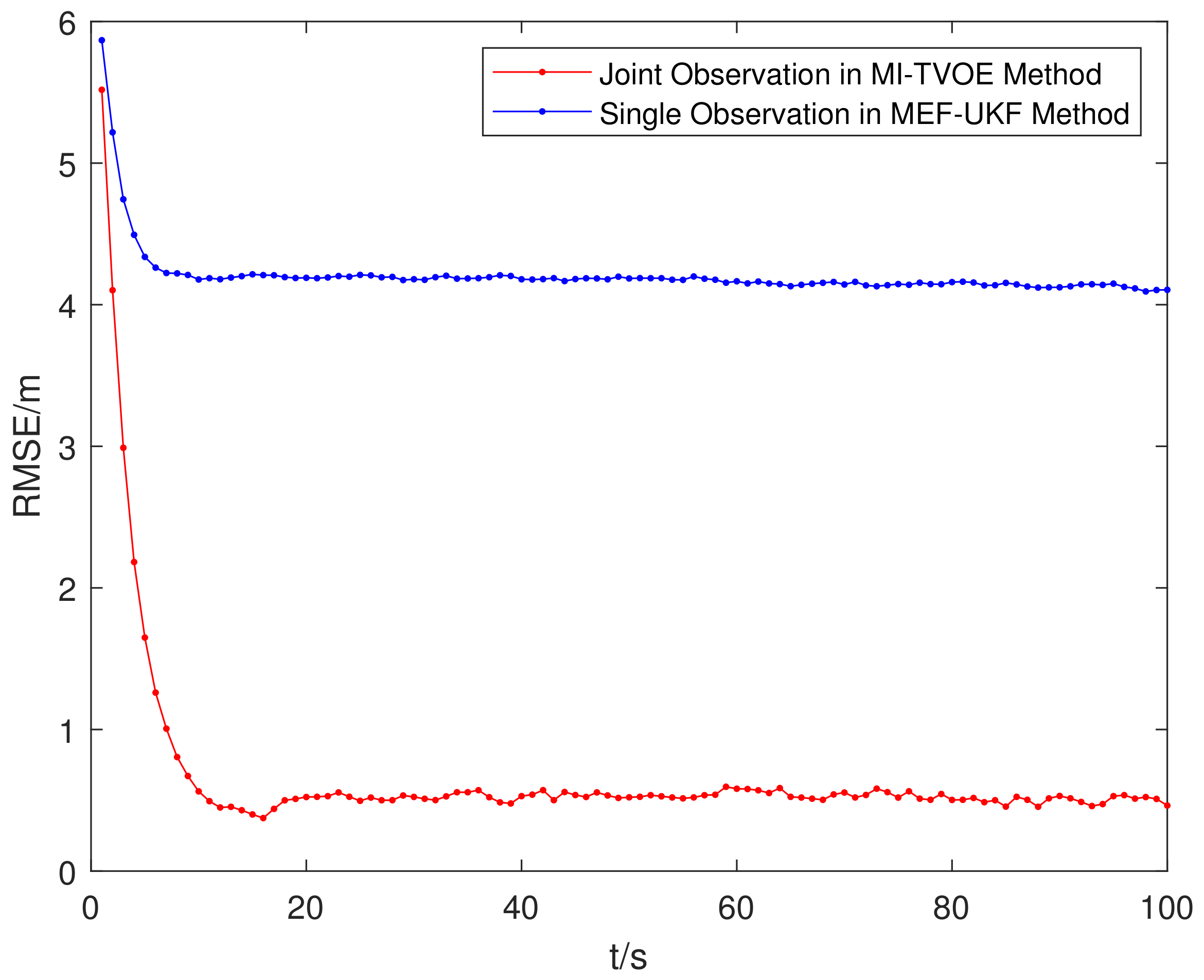
5.2.1. Tracking Result from Different Sensors

Figure 5 and Figure 6 show the tracking trajectory and the tracking RMSE from different sensors, respectively.

It can be seen from Figure 5 and Figure 6 that the tracking result obtained from each sensor is less accurate than that of the proposed MI-TVOE algorithm, since the MI-TVOE algorithm can fuse the tracking results from different sensors with time-varying observation error, which increases the vehicle tracking accuracy.

In this paper, three sensors are used for simulation. If one of the sensors does not receive a signal, the vehicle can also be tracked by fusing the other two sensors interactively. If one of the sensors has a large observation noise, the MI-TVOE algorithm in this paper can still handle the large noise well. Suppose that sensor B fails and has a large observation-noise covariance, as shown in

Table 3. The observation error for sensor B.

Model	Error Model1	Error Model2	Error Model3
Parameter	$d_{21}={13}^2$ $a_{21}={\left(\frac{1}{57.3}\right)}^2$ $r_{21}={10}^2$	$d_{22}={12}^2$ $a_{22}={\left(\frac{2}{57.3}\right)}^2$ $r_{22}={20}^2$	$d_{23}=3^2$ $a_{23}={\left(\frac{0.35}{57.3}\right)}^2$ $r_{23}={15}^2$

. Then, the tracking result from each sensor and the proposed MI-TVOE are as shown in Figure 7. It can be seen from Figure 7 that if sensor B fails and has a large observation noise, the tracking RMSE from sensor B will obviously be increased. However, the MI-TVOE algorithm in this paper still has a good tracking performance, which demonstrates its robustness for a large-noise environment.

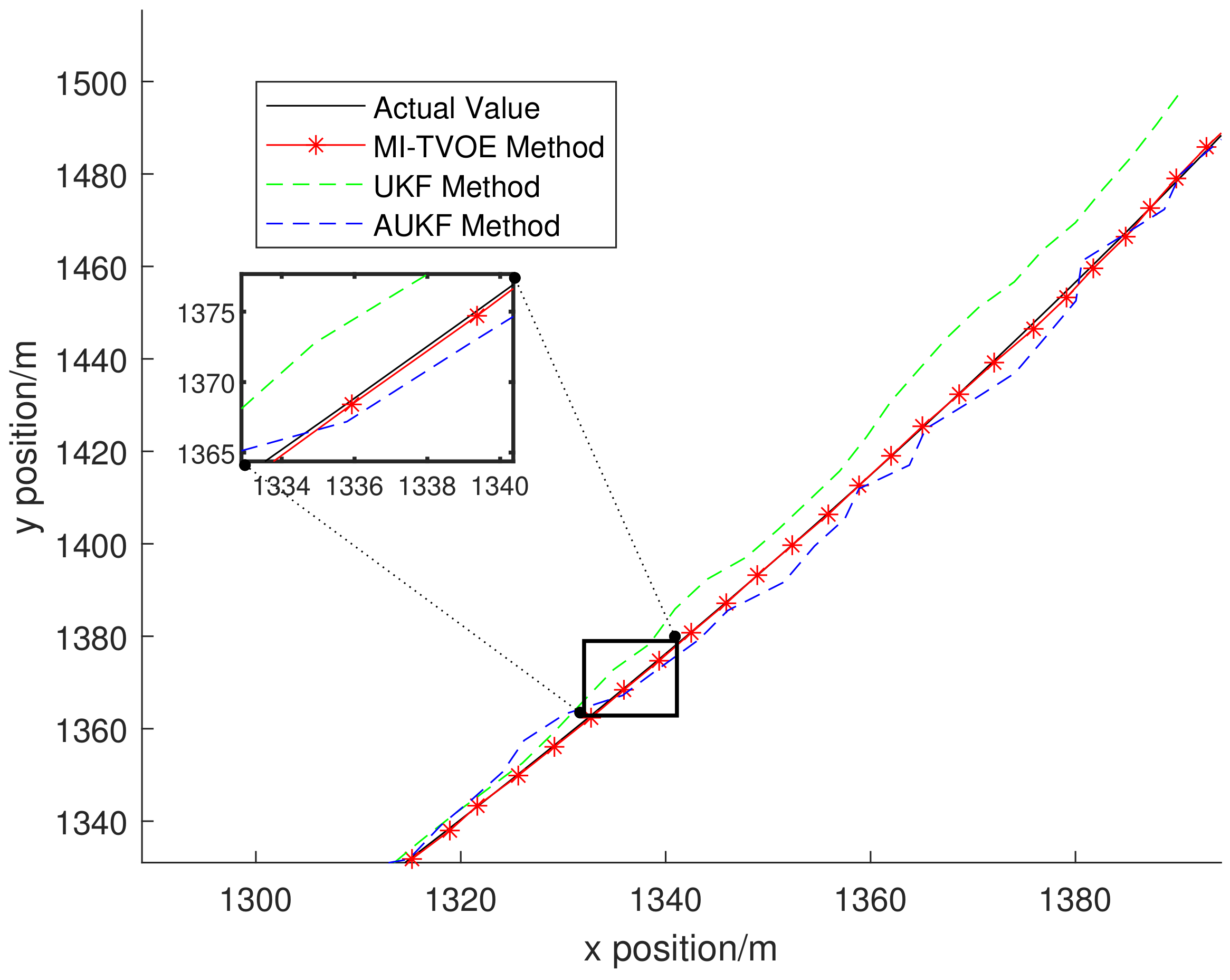
5.2.2. Tracking Result from Different Algorithm

In Figure 8 and Figure 9, we compare the proposed MI-TVOE algorithm with the AUKF algorithm, and UKF algorithm when the observation error is time varying.

From Figure 8 and Figure 9, we can see that, the UKF method has the lowest accuracy than the other two algorithms and the tracking result from UKF method is divergent when the observation error is time varying. The accuracy of the proposed MI-TVOE algorithm is higher than AUKF method since the proposed MI-TVOE algorithm can predict the statistic information of time-varying observation error and fuse the tracking result from each sensor, which significantly improves the tracking accuracy.

Figure 10 and Figure 11 show the comparison of tracking trajectory and tracking RMSE with MEF-UKF method [34] and the proposed MI-TVOE algorithm. The MEF-UKF method only uses distance observation with time-varying observation error, while the proposed MI-TVOE algorithm uses the jointed observation matrix with distance, angle, and Doppler information.

From Figure 10 and Figure 11, we can see that the proposed MI-TVOE algorithm obviously increases the tracking accuracy, since it uses the jointed observation information. Moreover, Figure 11 clearly shows that the tracking error for MI-TVOE algorithm with jointed observation information also has a faster convergence than the MEF-UKF method with single observation.

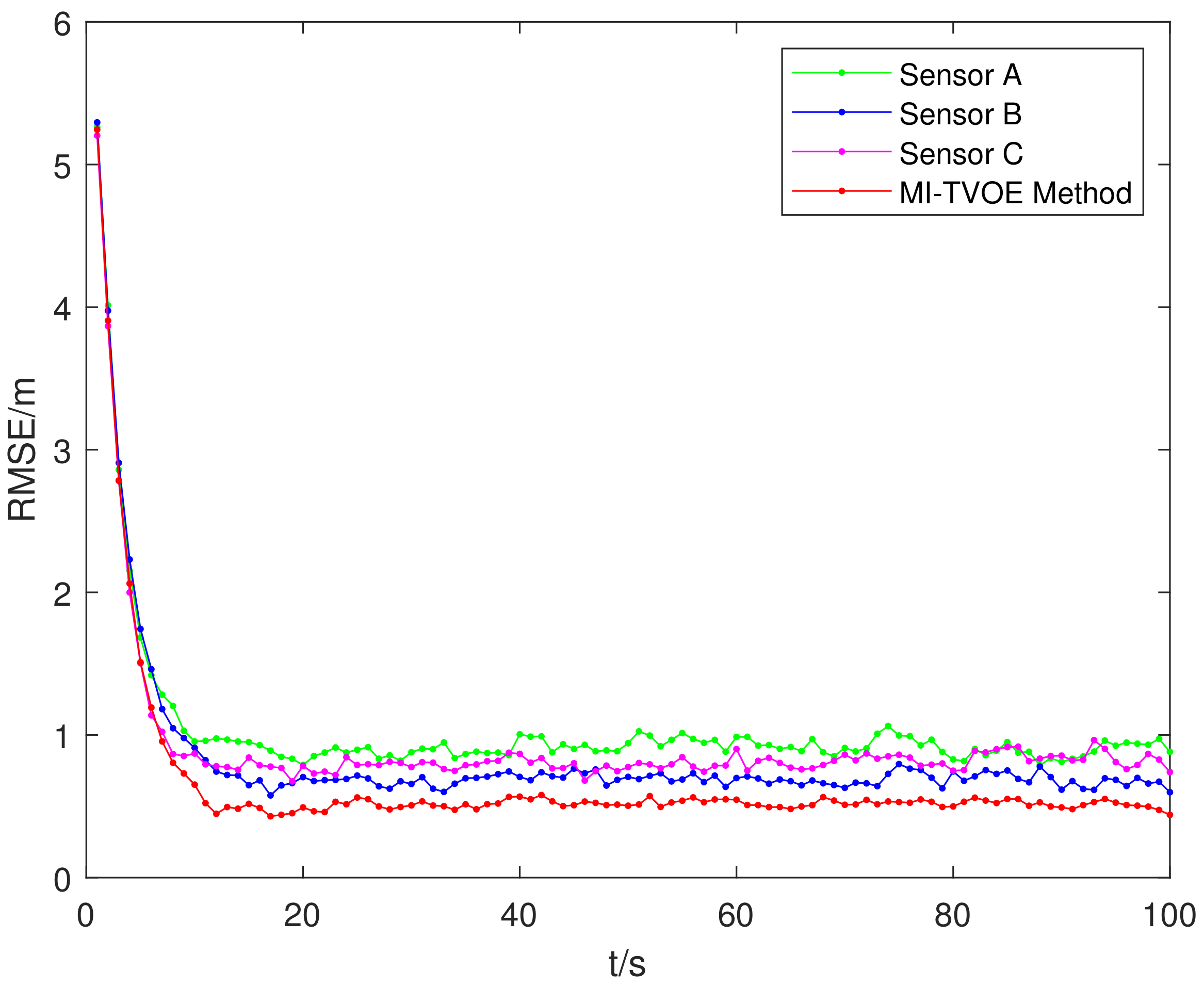
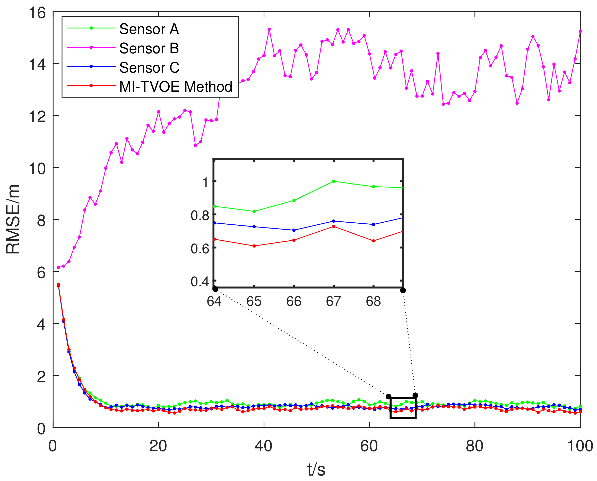
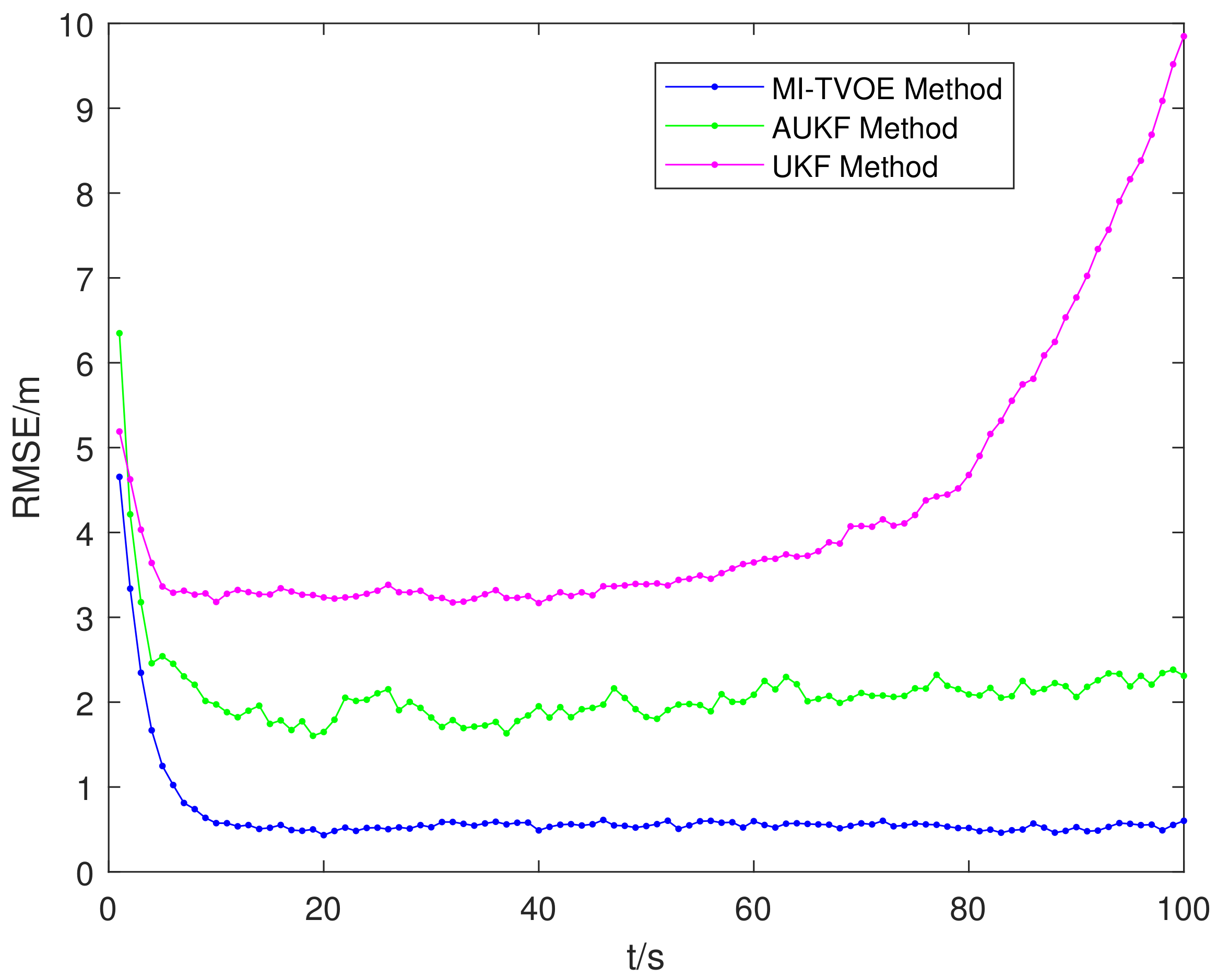
5.2.3. Tracking Performance Analysis

Table 4. Comparison of RMSE(m) with different algorithm.

Algorithm	Sensor A	Sensor B	Sensor C	Fusion
Traditional UKF method	5.4794	5.1668	5.2910
MEF-UKF method	4.3258	4..2050	4.2608
MI-TVOE method	1.0331	0.8532	0.9146	0.6630

lists the tracking RMSE from different algorithm.

Table 4 illustrates that when multiple sensors are simultaneously observing, the time-varying error model under multi-variate observation can significantly improve the tracking accuracy of moving vehicles. Compared with a traditional UKF method, the tracking accuracy of the MI-TVOE method in this paper is improved by 87.9%, which is more suitable for real tracking scenarios and has better robustness.

5.2.4. Computational Complexity Analysis

During the positioning process, due to the time varying and uncertainty of the positioning environment, the observation accuracy will also change with time, which is unknown and random. The VB algorithm can solve this problem well, but its complexity linearly increases with the product of the number of variables and the number of iterations. If there are many non-deterministic variables with potential statistical information in the system, the complexity of the algorithm is also high. However, the MI-TVOE algorithm proposed in this paper is only related to the number of error models, which significantly reduces the computational complexity.

6. Experimental Result

In this section, we will design a tracking experiment for an Unmanned Mobile Platform in an outdoor parking lot and give the experimental results of the proposed MI-TVOE algorithm to analyze and demonstrate its performance. In this paper, we will compare the tracking result between the proposed MI-TVOE algorithm and the algorithm in [35]. In [35], the author proposed an inertial navigation and Kalman-filter-based positioning algorithm, which is referred to as INS+KF. This algorithm uses the INS to obtain the speed, acceleration, and other information of the moving target in real time. Then, the positioning data are obtained by using time difference of arrival (TDOA) and the Gauss–Newton (GN) method. Finally, the Kalman filter is used to track the mobile target.

6.1. Experiment Settings

In this paper, we use a four-wheel omni-directional vehicle as a mobile platform that is shown in Figure 12.

Table 5. The specifications of the mobile platform.

Features	Parameter
Dimensions	450 × 330 × 115 mm
Drive mode	Four-wheel independent drive
Rated load capacity	20 kg
Maximum movement speed	0.75 m/s
Maximum rotation speed	215 °/s
Adapted terrain	Indoor and outdoor cement pavement with less pits

lists the main specifications of the mobile platform. Meanwhile, we use MTi-G-710 INS to capture the speed and the acceleration of mobile platform in real time. The ultra-wideband platform is used to send and receive information such as ranging and positioning.

Table 6. The specifications of the MTi-G-710 INS.

Feature	Parameter	Feature	Parameter
Input voltage	(4.5 V, 34 V)	Delay	<2 ms
Roll angle (static)	0.2°	Roll angle (dynamic)	0.3°
Sampling frequency	10 kHz/ch (60 kS/s)	Speed accuracy	0.05 m/s

and

Table 7. The specifications of the ultra-wideband platform.

Feature	Parameter
Size parameters	6 cm × 5.3 cm
Quality	12 g
Frequency Range	(3.5 GHz, 6.5 GHz)
Bit rate	Up to 6.8 Mbps

list the main specifications of the MTi-G-710 INS and ultra-wideband platform. The total station (TS) is used to measure the real position of the target and sensors. The experimental environment and the placement of equipment are shown in Figure 13. Three sensors are used for tracking in the experiment and the coordinates of the sensors are shown in

Table 8. The coordinates of three sensors.

Sensor	X(m)	Y(m)
Sensor A	14.1531	0.6864
Sensor B	1.7520	7.9625
Sensor C	0	0

.

6.2. Experimental Results Analysis

We compare the proposed MI-TVOE algorithm with the INS+KF algorithm. From Figure 14, we can see that the tracking trajectory of the MI-TVOE algorithm is closer to the real trajectory and the tracking result of MI-TVOE is more stable. The following experimental data were all obtained in a noise-changing environment.

In

Table 9. Tracking RMSE comparison between MI-TVOE and INS+KF.

Algorithm	INS+KF	MI-TVOE Method
RMSE (m)	0.0509	0.0314

, we compare the tracking RMSE between the two algorithms. It can be seen from Table 9 that the tracking error of the proposed MI-TVOE algorithm is 0.0195 m, which is lower than the INS+KF algorithm.

7. Conclusions

In this paper, we propose a multi-sensor interacted vehicle-tracking algorithm with time-varying observation error. Firstly, we propose a time-varying and jointed-observation error model to indicate the changing measurement noise. Then, a multi-sensor interacted vehicle-tracking algorithm is proposed to predict the statistical information of time-varying observation error and provide a global tracking result by fusing the time-varying observation information from different sensors. In the complex tracking scenes, the proposed MI-TVOE algorithm not only improves the tracking performance with robustness, but also reduces the computational complexity with time-varying observation error. In addition, by comparing the proposed MI-TVOE algorithm with the single-sensor-based tracking method, the traditional UKF method, the AUKF method and the MEF-UKF method, it is shown that the MI-TVOE algorithm can improve the tracking accuracy significantly in a complex environment with time-varying observation noise. Although the MI-TVOE method has a good improvement in tracking accuracy, it is only for single-vehicle tracking. In the future, we will solve the joint tracking problem with multiple vehicles in more complex and changing environments.

References

1. Fang, Y.; Wang, W.; Yan, X.; Zhao, H.; Zha, H. On-Road Vehicle Tracking Using Part-Based Particle Filter. IEEE Trans. Intell. Transp. Syst. 2019, 20, 4538–4552. [Google Scholar] [CrossRef]
2. Sun, C.; Zhang, X.; Zhou, Q.; Tian, Y. A Model Predictive Controller with Switched Tracking Error for Autonomous Vehicle Path Tracking. IEEE Access 2019, 7, 53103–53114. [Google Scholar] [CrossRef]
3. Zhang, B.; Zong, C.; Chen, G.; Zhang, B. Electrical Vehicle Path Tracking Based Model Predictive Control with a Laguerre Function and Exponential Weight. IEEE Access 2019, 7, 17082–17097. [Google Scholar] [CrossRef]
4. Scheunert, U.; Cramer, H.; Fardi, B.; Wanielik, G. Multi sensor based tracking of pedestrians: A survey of suitable movement models. In Proceedings of the IEEE Intelligent Vehicles Symposium, Parma, Italy, 14–17 June 2004; pp. 774–778. [Google Scholar]
5. Deming, R.; Schindler, J.; Perlovsky, L. Multi-Target/Multi-Sensor Tracking Using Only Range and Doppler Measurements. IEEE Trans. Aerosp. Electron. Syst. 2009, 45, 593–611. [Google Scholar] [CrossRef]
6. Ding, X.; Wang, Z.; Zhang, L.; Wang, C. Longitudinal Vehicle Speed Estimation for Four-Wheel-Independently-Actuated Electric Vehicles Based on Multi-Sensor Fusion. IEEE Trans. Veh. Technol. 2020, 69, 12797–12806. [Google Scholar] [CrossRef]
7. Yang, P.; Duan, D.; Chen, C.; Cheng, X.; Yang, L. Multi-Sensor Multi-Vehicle (MSMV) Localization and Mobility Tracking for Autonomous Driving. IEEE Trans. Veh. Technol. 2020, 69, 14355–14364. [Google Scholar] [CrossRef]
8. Tian, B.; Li, Y.; Li, B.; Wen, D. Rear-View Vehicle Detection and Tracking by Combining Multiple Parts for Complex Urban Surveillance. IEEE Trans. Intell. Transp. Syst. 2014, 15, 597–606. [Google Scholar] [CrossRef]
9. Zheng, J.; Yu, H.; Wang, S.; Long, Y.; Meng, F. Distributed adaptive multi-sensor multi-target tracking algorithm. J. Chin. Inert. Technol. 2015, 23, 472–476. [Google Scholar]
10. Yomchinda, T. A method of multirate sensor fusion for target tracking and localization using extended Kalman Filter. In Proceedings of the 2017 Fourth Asian Conference on Defence Technology—Japan (ACDT), Tokyo, Japan, 29 November–1 December 2017; pp. 1–7. [Google Scholar]
11. Hu, F.; Wu, G. Distributed Error Correction of EKF Algorithm in Multi-Sensor Fusion Localization Model. IEEE Access 2020, 8, 93211–93218. [Google Scholar] [CrossRef]
12. Yang, F.; Tang, W.; Wang, Y.; Chen, S. A RANSAC-Based Track Initialization Algorithm for Multi-Sensor Tracking System. In Proceedings of the 2018 International Conference on Control, Automation and Information Sciences (ICCAIS), Hangzhou, China, 24–27 October 2018; pp. 96–101. [Google Scholar]
13. Shi, Y.; Yang, Z.; Zhang, T.; Lin, N.; Zhao, Y.; Zhao, Y. An Adaptive Track Fusion Method with Unscented Kalman Filter. In Proceedings of the 2018 IEEE International Conference on Smart Internet of Things (SmartIoT), Xi’an, China, 17–19 August 2018; pp. 250–254. [Google Scholar]
14. Zhou, N.; Lau, L.; Bai, R.; Moore, T. A Genetic Optimization Resampling Based Particle Filtering Algorithm for Indoor Target Tracking. Remote Sens. 2021, 13, 132. [Google Scholar] [CrossRef]
15. Niknejad, H.T.; Takeuchi, A.; Mita, S.; McAllester, D. On-road multivehicle tracking using deformable object model and particle filter with improved likelihood estimation. IEEE Trans. Intell. Transp. Syst. 2012, 13, 748–758. [Google Scholar] [CrossRef]
16. Xu, H.; Bai, X.; Liu, P.; Shi, Y. Hierarchical Fusion Estimation for WSNs with Link Failures Based on Kalman-Consensus Filtering and Covariance Intersection. In Proceedings of the 2020 39th Chinese Control Conference (CCC), Shenyang, China, 27–29 July 2020; pp. 5150–5154. [Google Scholar]
17. Li, X.; Wu, P.; Zhang, X. An interacting multiple models probabilistic data association algorithm for maneuvering target tracking in clutter. Int. Symp. Comput. Inform. 2015, 13, 1685–1692. [Google Scholar]
18. Zhu, L.; Cheng, X. High manoeuvre target tracking in coordinated turns. IET Radar Sonar Navig. 2015, 9, 1078–1087. [Google Scholar] [CrossRef]
19. Choi, W.Y.; Kang, C.M.; Lee, S.H.; Chung, C.C. Radar accuracy modeling and its application to object vehicle tracking. Int. J. Control Autom. Syst. 2020, 18, 3146–3158. [Google Scholar] [CrossRef]
20. Li, Z.; Zhang, H.; Zhou, Q.; Che, H. An Adaptive Low-Cost INS/GNSS Tightly-Coupled Integration Architecture Based on Redundant Measurement Noise Covariance Estimation. Sensors 2017, 17, 2032. [Google Scholar] [CrossRef] [Green Version]
21. Akhlaghi, S.; Zhou, N.; Huang, Z. Adaptive adjustment of noise covariance in Kalman filter for dynamic state estimation. In Proceedings of the 2017 IEEE Power $ Energy Society General Meeting, Chicago, IL, USA, 16–20 July 2017; pp. 1–5. [Google Scholar]
22. Sun, Y.; Jing, F.; Liang, Z.; Tan, M. MMSE State Estimation Approach for Linear Discrete-Time Systems With Time-Delay and Multi-Error Measurements. IEEE Trans. Autom. Control 2017, 62, 1530–1536. [Google Scholar] [CrossRef]
23. Jamroz, B.F.; Williams, D.F.; Rezac, J.D.; Frey, M.; Koepke, A.A. Accurate Monte Carlo Uncertainty Analysis for Multiple Measurements of Microwave Systems. In Proceedings of the 2019 IEEE MTT-S International Microwave Symposium (IMS), Boston, MA, USA, 2–7 June 2019; pp. 1279–1282. [Google Scholar]
24. Lin, P.; Hu, C.; Lou, Y. Distributed Variational Bayes Based on Consensus of Probability Densities. In Proceedings of the 2020 39th Chinese Control Conference (CCC), Shenyang, China, 27–29 July 2020; pp. 5013–5018. [Google Scholar]
25. He, W.; Liu, Y.; Yao, H.; Mai, T.; Zhang, N.; Yu, F.R. Distributed Variational Bayes-Based In-Network Security for the Internet of Things. IEEE Internet Things J. 2021, 8, 6293–6304. [Google Scholar] [CrossRef]
26. Kheirandish, A.; Fatehi, A.; Gheibi, M.S. Identification of Slow-Rate Integrated Measurement Systems Using Expectation–Maximization Algorithm. IEEE Trans. Instrum. Meas. 2020, 69, 9477–9484. [Google Scholar] [CrossRef]
27. Peng, Y.; Panlong, W.; Shan, H. An IMM-VB Algorithm for Hypersonic Vehicle Tracking with Heavy Tailed Measurement Noise. In Proceedings of the 2018 International Conference on Control, Automation and Information Sciences (ICCAIS), Hangzhou, China, 24–27 October 2018; pp. 169–174. [Google Scholar]
28. Li, Z.; Zhang, J.; Wang, J.; Zhou, Q. Recursive Noise Adaptive Extended Object Tracking by Variational Bayesian Approximation. IEEE Access 2019, 7, 151168–151179. [Google Scholar] [CrossRef]
29. Byeon, M.; Lee, M.; Kim, K.; Choi, J.Y. Variational inference for 3-D localization and tracking of multiple targets using multiple cameras. IEEE Trans. Neural Netw. Learn. Syst. 2019, 30, 3260–3274. [Google Scholar] [CrossRef]
30. Stauffer, C.; Grimson, W.E.L. Learning patterns of activity using real-time tracking. IEEE Trans. Pattern Anal. Mach. Intell. 2000, 22, 747–757. [Google Scholar] [CrossRef] [Green Version]
31. Wang, G.; Wu, J.; Li, X.; Mo, R.; Zhang, M. A real-time tracking prediction for maneuvering target. In Proceedings of the 2018 Chinese Control And Decision Conference (CCDC), Shenyang, China, 9–11 June 2018; pp. 3562–3566. [Google Scholar]
32. Zhang, J.; Chen, T.; Shi, Z. A Real-Time Visual Tracking for Unmanned Aerial Vehicles with Dynamic Window. In Proceedings of the 2020 China Semiconductor Technology International Conference (CSTIC), Shanghai, China, 26 June–17 July 2020; pp. 1–3. [Google Scholar]
33. Yan, X. Research and Design of Positioning Method of Small Unmanned Mobile Platform Based on UWB; Chang’an University: Xi’an, China, 2020. (In Chinese) [Google Scholar]
34. Zhang, Q.; Gao, J.; Sun, H. The Unscented Kalman Filter Based Fusion Tracking Method with Multi-error Model. In Proceedings of the 2021 IEEE International Conference on Signal Processing, Communications and Computing (ICSPCC), Xi’an, China, 17–19 August 2021; pp. 1–5. [Google Scholar]
35. Julier, S.J.; Uhlmann, J.K. Unscented filtering and nonlinear estimation. Proc. IEEE 2004, 92, 401–422. [Google Scholar] [CrossRef] [Green Version]
Figure 1. The structure of tracking system.
Remotesensing 14 02176 g001
Figure 2. Block diagram of the proposed algorithm.
Remotesensing 14 02176 g002
Figure 3. The flow chart of the algorithm.
Remotesensing 14 02176 g003
Figure 4. The real trajectory of the moving vehicle and the location of three sensors.
Remotesensing 14 02176 g004
Figure 5. Tracking trajectory from different sensors.
Remotesensing 14 02176 g005
Figure 6. Tracking RMSE from different sensors.
Remotesensing 14 02176 g006
Figure 7. Tracking RMSE from sensors B and other sensors.
Remotesensing 14 02176 g007
Figure 8. Tracking trajectory comparison between MI-TVOE, AUKF and UKF.
Remotesensing 14 02176 g008
Figure 9. Tracking RMSE comparison between MI-TVOE, AUKF and UKF.
Remotesensing 14 02176 g009
Figure 10. Tracking trajectory comparison between MI-TVOE and MEF-UKF.
Remotesensing 14 02176 g010
Figure 11. Tracking RMSE comparison between MI-TVOE and MEF-UKF.
Remotesensing 14 02176 g011
Figure 12. The unmanned mobile platform.
Remotesensing 14 02176 g012
Figure 13. Experimental environment.
Remotesensing 14 02176 g013
Figure 14. Tracking trajectory comparison between MI-TVOE and INS+KF.
Remotesensing 14 02176 g014