Article

Monitoring Light Pollution with an Unmanned Aerial Vehicle: A Case Study Comparing RGB Images and Night Ground Brightness

1
Istituto per la BioEconomia del Consiglio Nazionale delle Ricerche, IBE–CNR, 50019 Sesto Fiorentino, FI, Italy
2
Istituto di Fisiologia Clinica del Consiglio Nazionale delle Ricerche, IFC–CNR, 56124 Pisa, PI, Italy
3
Istituto di Scienze Marine del Consiglio Nazionale delle Ricerche, ISMAR–CNR, 19032 Lerici, SP, Italy
*
Author to whom correspondence should be addressed.
Remote Sens. 2022, 14(9), 2052; https://doi.org/10.3390/rs14092052
Submission received: 11 March 2022 / Revised: 15 April 2022 / Accepted: 22 April 2022 / Published: 25 April 2022
(This article belongs to the Special Issue UAV Photogrammetry for Environmental Monitoring)

Abstract

:
There are several tools and methods to quantify light pollution due to direct or reflected light emitted towards the sky. Unmanned aerial vehicles (UAV) are still rarely used in light pollution studies. In this study, a digital camera and a sky quality meter mounted on a UAV have been used to study the relationship between indices computed on night images and night ground brightness (NGB) measured by an optical device pointed downward towards the ground. Both measurements were taken simultaneously during flights at an altitude of 70 and 100 m, and with varying exposure time. NGB correlated significantly both with the brightness index (−0.49 ÷ −0.56) and with red (−0.52 ÷ −0.58) and green band indices (−0.42 ÷ −0.58). A linear regression model based on the luminous intensity index was able to estimate observed NGB with an RMSE varying between 0.21 and 0.46 mpsas. Multispectral analysis applied to images taken at 70 m showed that increasing exposure time might cause a saturation of the colors of the image, especially in the red band, that worsens the correlation between image indices and NGB. Our study suggests that the combined use of low cost devices such as UAV and a sky quality meter can be used for assessing hotspot areas of light pollution originating from the surface.

1. Introduction

The excessive use of night illumination causes light pollution. Despite the use of systems that cut off part of the upward emissions, light pollution is increasing [1]. Moreover, the use of more efficient lighting technology (e.g., LED) might have a negative rebound effect, such as the temptation of investing cost savings produced by this technology in new illumination systems even if they are not necessary [2]. Light pollution has several negative consequences on the quality of the night sky that might limit star visibility [3,4], and on terrestrial and marine species [5,6,7,8,9,10,11,12,13,14] including plants [15,16,17,18,19,20] and humans [21,22,23].
Monitoring light pollution is a key issue and a difficult task to perform due to the low intensity of the signal and its spatial variability. Several approaches are available from satellite remote sensing for spatial variation [24,25,26,27], to ground measurement with meters (e.g., SQM and TESS-W) used in stationary monitoring networks [28,29,30,31,32,33] and moving campaigns [25,34], and DSLR cameras for assessing light pollution variability above a specific location [35,36,37,38,39]. Some studies have highlighted limitations due to the spectral characteristics of sky quality meters (SQMs) that make the conversion from magnitude to radiance difficult [40], the ageing of the system that might affect measurements [41] and differences in the angular response on sky-brightness measurements [42]. Despite these limitations, this sensor is still widely used in the scientific community and it is currently used for monitoring light pollution both by scientific institutions and regional services [29,30,31,32,33,43].
This information is coupled in models that are used to produce maps of light pollution such as the World Atlas of Light Pollution [44]. Actually, both satellite images and modeled maps have a good but limited spatial resolution for characterizing urban and peri-urban areas that are characterized by a high spatial variability of artificial light at night. Most of these studies are based on ground-based measurements from the point of view of the human eye, while a few of them, apart from studies based on satellite images or photographs from the International Space Station [26,45], have tried to study artificial light diffusion based on observations from the sky. For instance, such a perspective could be of interest in the assessment of an outdoor lighting installation in terms of upward light emissions and the consequent light pollution. However, the partial obstruction of artificial light due to urban features, such as trees and buildings, might affect the reliability of this information as a consequence of the anisotropic diffusion of artificial light. The effect of anisotropy has been considered in a correlation study between satellite images and lighting systems [46] and in a case study aimed to quantify this effect in a case study [47].
Unmanned aerial vehicle (UAV) systems, also known as drones, are now very popular tools for monitoring the environment in scientific disciplines such as agriculture [48], forestry [49], coastal and beach dynamics [50], marine litter accumulation along the coast [51,52,53] and even in citizen science projects [54,55]. However they are still poorly used in light pollution studies. Light pollution occurs due to scattering of the direct component of outdoor lighting emitted towards the sky and the reflected component by lit surfaces. Although these emissions should be quantified during the design of outdoor lighting, there is not yet a recognized standard either for the methodology or the instrumentation for the assessment of light pollution [56]. Drones have been suggested as tools for monitoring and assessing light pollution from the air [26,57,58]. However, issues such as the cost of equipment, the limited payload that can be carried by the drone and the range of a single flight still limit the use of such systems in this research field. Indeed, legal restrictions on the height of flight and the short temporal autonomy limit the possibility of monitoring large areas. On the other hand, low altitude flight enables the capture of high resolution information on the spatial variability of ground brightness. Some studies have compared the use of ground-based measurements with digital cameras, airborne measurements with satellite images and detailed airborne measurements with UAV images for the assessment of light pollution from different points of view [59]. UAV nocturnal images combined with VIIRS satellite images have also been used to estimate population density [60]. Bouroussis and Topalis [56] proposed the use of a digital camera mounted on a drone for assessing lighting installations from different points of view in the three dimensional space, taking advantage of the UAV’s capability to easily program trajectories of any form and point of acquisition along the route. Some attempts to compare the information of aerial images taken by UAVs and measures of light pollution have already been made. In a previous study, the effect of a single and isolated luminaire, with and without a mask for upward radiation cutoff on the surrounding environment, was assessed by recording the illuminance on the ground and at a 14-m level, by using an illuminance meter mounted on a drone and a mobile one on the ground [61].
In other studies, city light dynamics through the night were monitored in urban areas, by using a digital camera mounted on a drone for acquiring aerial images of the night illumination of the area, while ground-based measurements on the same area were recorded by SQM devices mounted on shopping carts [62] or cars [63]. Sometimes, comparisons between aerial images and SQM measurements were made by using indices calculated on the red-green-blue component of the images [63]. Even though sky quality meters were designed to measure diffused light on the sky by astronomers, they have also been used to measure ground brightness in other studies [25]. However, to the best of our knowledge, the use of SQM for estimating light pollution from drones has not been performed yet.
The aim of this study is to present a low cost system for monitoring light pollution that is composed of an unmanned aerial vehicle equipped with a digital camera and an optical sensor for measuring the surface brightness of an area. This system is used to investigate the surface brightness variability in a real context. A small urbanized area was monitored with flights at different altitudes, with a digital camera and an optical sensor (sky quality meter or SQM) oriented downwards to the nadir. Night images in RAW format and SQM measurements were taken simultaneously on the selected area. The first aim of the study was to investigate if SQMs, which are devices designed to measure the diffused brightness of the sky, can also be used to monitor the brightness of ground surfaces from different altitudes (SQM measurements taken from the sky are referred to here as “night ground brightness” or NGB). Image indices and NGB measurements, used as proxies of the brightness due to the light emitted by luminaires and reflected by the ground, were compared to assess the relationship between these two types of information. We assume that brighter areas on the images are a reliable indicator of hotspot areas of light pollution directed upward. Therefore, we used indices calculated on the images as a proxy for the light emitted towards the sky and compared them with measurements taken by the SQM. Overall, the study is designed to provide useful information and recommendations for more extensive future assessment of the capability of low cost devices mounted on a UAV for identifying light pollution sources from the sky. Moreover, SQMs or optical sensors with similar characteristics, specifically designed for their use on UAV, could be tools that easily provide information on the spatial distribution of surface brightness—which in turn can be used to identify areas characterized by higher levels of upward light emission.

2. Materials and Methods
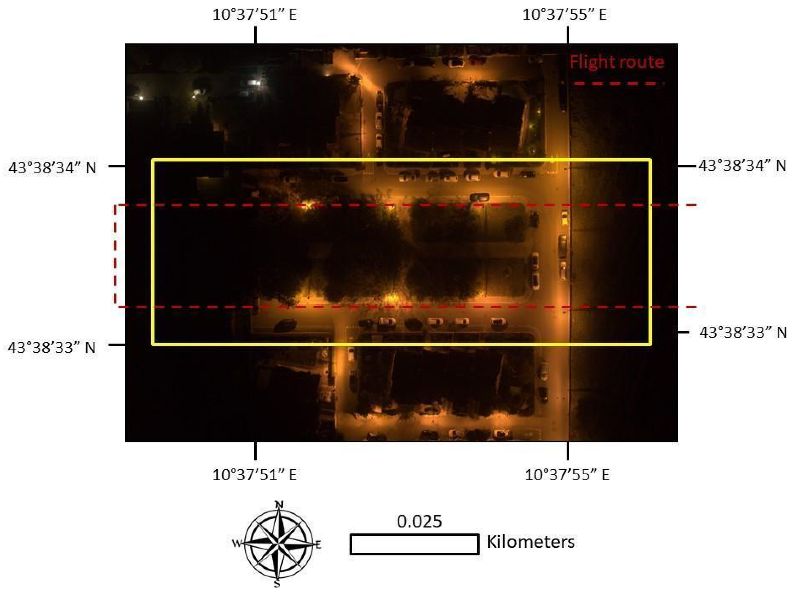
2.1. Study Area

Our study area was located in a countryside and residential area in the province of Pisa, Italy (Figure 1). The study area was approximately a rectangle, with an area size of about 1 hectare. This area includes houses, roads and green areas. The public illumination system of this area is mainly composed of HPS amber lights (n = 16) and only a few white lights (n = 3). The studied area is an urbanized area surrounded by countryside with a sudden transition between dark and lit areas at the borders. We chose this area because it is characterised by different levels of surface brightness and its dimensions were suitable for the limitations imposed by the flight autonomy of the drone, which was further limited by the presence of the SQM on board.

2.2. UAV Characteristics

We used a Phantom 4 PRO V.2, a commercial UAV suitable for this type of application, thanks to the good resolution of the camera, the compactness of the aircraft, the flight stability and the possibility of carrying a light sensor (Figure 2).
It has a titanium and magnesium alloy structure, increasing the strength of its frame and reducing its weight; together with a good battery capacity (5870 mA). These features allow a flight time of up to approximately 30 min. It has a gimbal three-axis stabilized camera with a 1-inch 20-megapixel CMOS sensor, capable of shooting up to 4 K/60 fps video and photo bursts, at up to 14 fps.
The camera’s field of view is 84°, with 24 mm equivalent focal length, and diaphragm f/2.8 to f/11 with autofocus from 1 m to infinity. The mechanical shutter speed ranges from 8 to 1/2000 s, while with the electronic shutter speed ranges from 1/2000 s to 1/8000 s. ISO range for stills images is 100 to 3200 in auto, and 100 to 12,800 in manual. For video shot in automatic mode it is the same, while for manual mode videos it is up to 6400. Three image sizes are available: 3:2 (5472 × 3648), 4:3 (4864 × 3648), and 16:9 (5472 × 3078), providing output in different formats: JPEG, DNG (RAW), and JPEG + DNG. The pixel depth of the RGB components in the DNG (RAW) format is 16 bits, which provides a higher dynamic range than the 8-bit depth of the JPEG format used in other studies [62]. While commercial cameras have been used to measure light pollution previously, it is acknowledged that accurate calibration is needed to obtain precise values. This is still a complex task which is camera dependent, and there is not yet a recognized standard for this procedure [39,63,64,65]. In this study, we did not calibrate the drone camera; however, we used the RAW format that is recommended by other studies [39,65,66,67] since it provides more reliable information than JPEG format which is compressed.
The gimbal can vary its tilt between +30° and −90°. This allows it to capture photos perpendicular to the direction of flight. It was equipped with an HD video transmission device capable of reaching a maximum range of 7 km. The correct position management was obtained thanks to two satellite tracking systems: GPS and GLONASS. The use of UAVs for 3D mapping of the terrain or sites has the advantage of accessing utilities, such as waypoint mapping to identify the surveyed area and flight path planning and control, provided by third-party applications. A remote controller allowed a pilot to manage the flight of the UAV; a smartphone (or tablet) could be connected to the remote controller to view the camera, read the telemetry and enable automatic functions. The maximum speed was 72 km/h and the maximum control range was 7 km from the pilot.

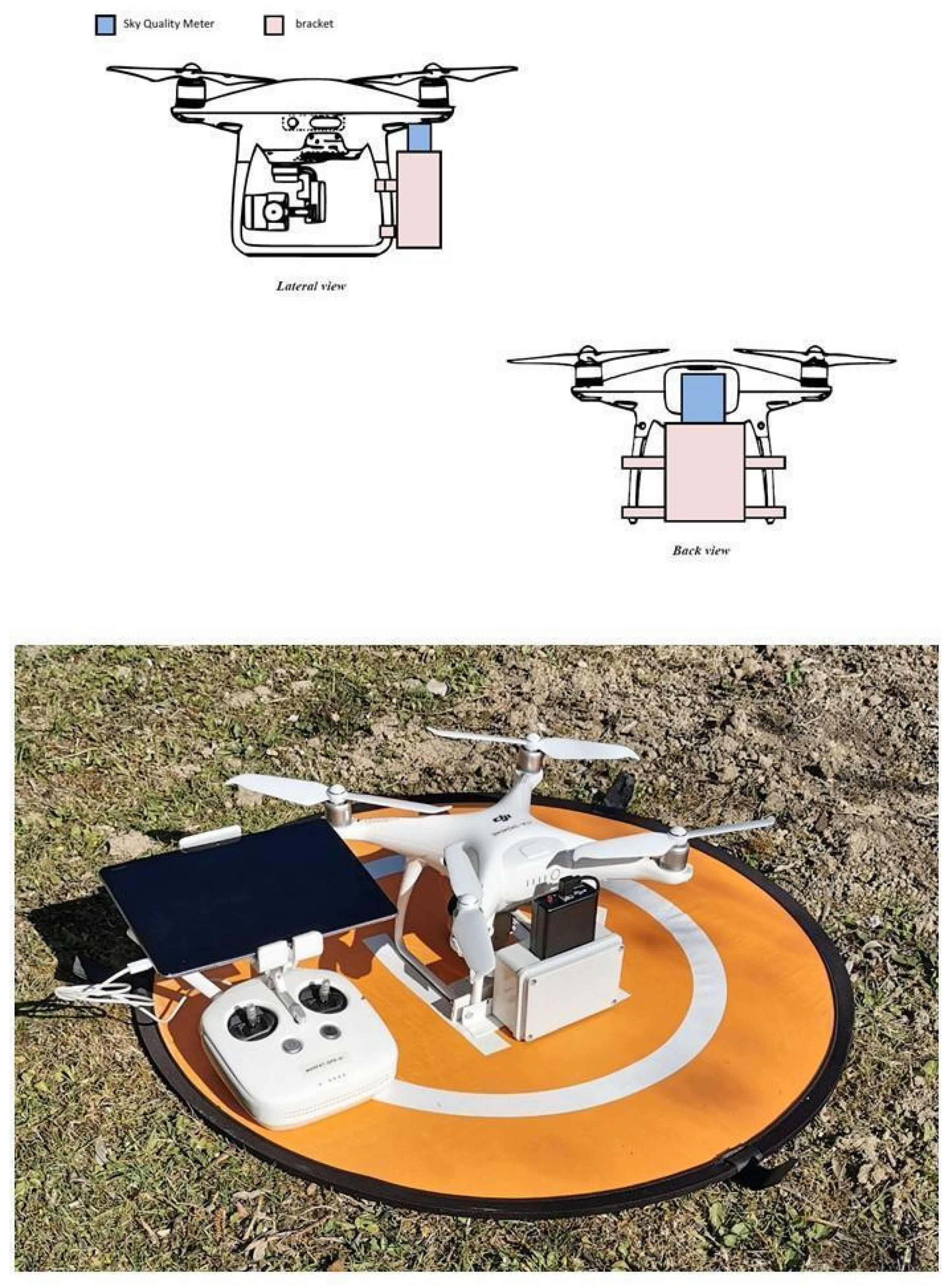
2.3. Light Pollution Sensor Mounted on the UAV

A model SQM-LU-DL Sky Quality Meter (SQM) by Unihedron (http://unihedron.com/, accessed on 21 April 2022) was attached to the rear side of the UAV via a bracket that contains the SQM’s power supply battery (Figure 2). The SQM measures surface brightness in magnitude/arcsec2 (mpsas). Normally this sensor is oriented upward towards the zenith and measures night sky brightness. In this study, the sensor is directed downward and perpendicularly to the ground, thus measuring the brightness of the luminaires and of the lit surfaces, which we refer to in this work as night ground brightness (NGB). We used the radiometric calibration of the SQM made by the manufacturer as in many other studies [25,28,29,30,31,32,33,63,68,69,70], even though some studies performed their own radiometric calibration [42,71].
Setting the SQM in the rear position produces an unbalanced flight attitude, but this is compensated by a sufficient level of thrust due to the power of the motors, and also offers the advantage of not hindering the visibility of the camera. The take-off was only performed in manual mode to compensate for the unbalance, which is not foreseen by the system in automatic mode. Subsequently, the flight can continue in automatic mode. In the future we plan to develop a more optimized support system for maintaining the correct flight attitude.

2.4. Device Settings

We chose two flight levels with altitudes of 70 and 100 metres, which gave us ground sampling distances of 1.92 cm and 2.74 cm respectively. Orthophotos were taken with the digital camera set to ISO 400 and an aperture of f/2.8. Other general settings were: mechanical shutter disabled, front led off, gimbal lock. The flight was managed in both manual and automatic modes, with the aim of maintaining a minimum overlap of 70%.
All flights were conducted over a segregated area devoid of people at that time. Three flight campaigns (six flights) were conducted over three nights with clear sky conditions (Table 1). The first two were conducted, respectively, at an altitude of 70 and 100 m on 3 April 2021 (A1, A2) and 23 April 2021 (B1, B2), setting the camera at a shutter speed of 1/6.25 s (160 ms), while the third flight was conducted at 70 m altitude using two different shutter speeds of ¼ s (250 ms) and ½ s (500 ms) in order to investigate the effect of exposure time on image saturation (C1, C2). At the beginning and the end of each single flight, the SQM was used to measure night sky brightness (NSB), in a dark location near the study area, by pointing it to the zenith.

2.5. Image Acquisition and Processing

The images were acquired in RAW mode, transferred to a PC and processed using AGISOFT METASHAPE Professional V. 1.6.1. Through this software we constructed the orthomosaic of the selected area. We derived the coordinates of the lampposts from Google Maps and we used them as marker points to geographically reference the orthomosaic map.

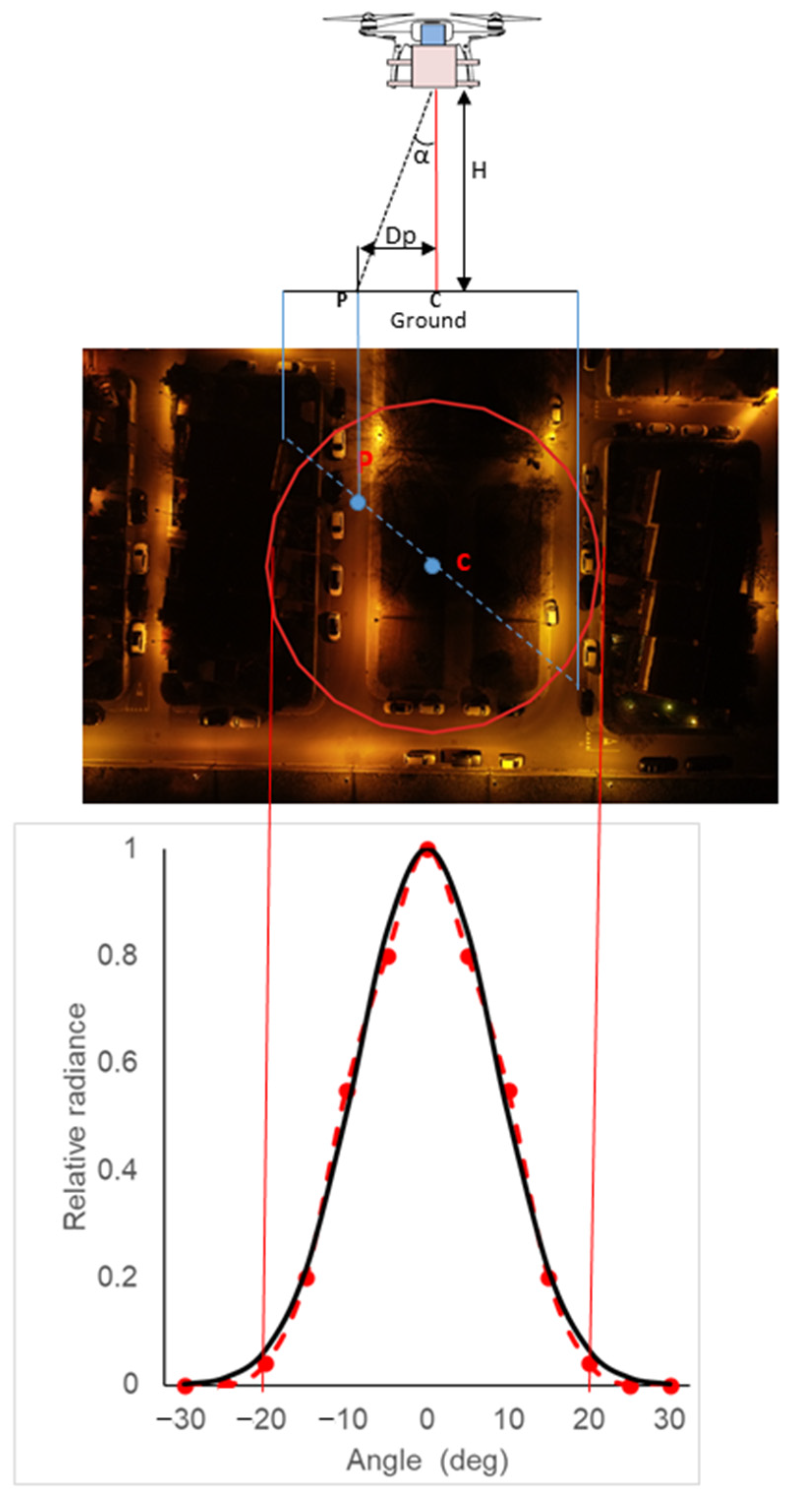
2.6. Relationship between UAV Image Indices and Night Sky Brightness

To compare the surface brightness of the scene captured by the UAV with the measures collected by the SQM, we used SQM response characteristics (relative radiance, referred to as rr) as reported in [72]. According to this study, the SQM has a maximum sensitivity in an FOV of 10° (rr between 0.5 and 1), while rr reduces to 10% for FOV between 10° and 20° and almost zero for angles higher than 20° (Figure 3). Therefore we considered the footprint of the SQM equal to the FOV of 20° centered on the point where the SQM took the measurement at 70 m and 100 m, also corresponding to the center of each orthophoto. This resulted in respective circles of 23.9 m and 34.2 m radius on each orthophoto (Figure 3). Then, for each pixel in the orthophoto we computed rr using the Formula (1) corresponding to the curve reported by Cinzano [72]:
rr = exp(−22.448 ∗ (arctan(Dp/H))2)
where H is the flight height, Dp is the distance of the pixel from the center of the image and 22.448 is a constant value set for obtaining the best approximation of the rr graph [72].
For each pixel of the orthophoto, we computed: red (R), green (G), blue (B) components and the brightness (I) taking into account the spectral sensitivity of the human eye that varies among the color bands (high in the green, low in the red and very low in the blue). Brightness (I) was calculated using, as weights of the RGB components, the luminous efficiency function by Poynton [73]:
I = 0.2125 ∗ R + 0.7154 ∗ G + 0.0721 ∗ B
Then, applying the relative radiance (rr) due to the FOV of the SQM, we calculated averaged indices of luminous intensity (Is), red (Rs), green (Gs) and blue (Bs) components for each orthophoto according the following formulas:
Is = log((⅀j(Ij ∗ rrj)/65356))
Rs = log((⅀j(Rj ∗ rrj)/65356))
Gs = log((⅀j(Gj ∗ rrj)/65356))
Bs = log((⅀j(Bj ∗ rrj)/65356))
The summation is normalized by dividing by 65536, which is the number of levels for RGB. The logarithm function was introduced to take into account that SQM measurements are expressed in magnitude/arcsec2 (mpsas) which is in logarithmic scale.

2.7. Statistical Analysis

Kendall rank correlation analysis between NGB and indices calculated on the orthophoto was performed on each dataset (A1, A2, B1 and B2). Linear regression models were calculated between NGB and the four indices for each dataset (A1,A2, B1,B2). The dataset where each model fit best was used as a training set (A2 in our study). Therefore we obtained four linear models for each index (Is, Rs, Gs, Bs). These models were then applied to estimate NGB values for the other three datasets (A1, B1, B2) that were used as validation sets. Estimated NGBs (Lis, Lrs, Lgs, Lbs) are computed by the following formula:
Lis = ai + bi ∗ Is
Lrs = ar + br ∗ Rs
Lgs = ag + bg ∗ Gs
Lbs = ab + bb ∗ Bs
where ax and bx coefficients are calculated on the training set (A2).
The performance of the linear regression model was calculated by evaluating mean error (ME) and root mean square error (RMSE) between estimated NGB (Lis, Lrs, Lgs, Lbs) and measured NGB values (Lo). For instance, ME and RMSE on Is were computed as:
ME = ⅀i(Lis − Lo)/n
RMSE = sqrt((⅀i(Lis − Lo)2)/n)
where n is the number of night images for each set.
All the analyses were conducted using R and Microsoft Excel.

2.8. Analysis of Orthophoto in Multispectral RGB

To appreciate the dynamic range of the images, distribution of pixels in multispectral RGB was analyzed. Red, green and blue digital numbers were normalized for the number of levels of the information (n = 65,536). For brightness (I), red (R), green (G) and blue (B) bands of each image, we calculated the percentage of pixels below the detection level (e.g., I = 0, Q0), the first quartile (e.g., 0 < I ≤ 0.25, Q1), the second quartile (e.g., 0.25 < I ≤ 0.50, Q2), the third quartile (e.g., 0.50 < I ≤ 0.75, Q3), the fourth quartile (e.g., 0.75 < I < 1, Q4) and the saturated pixels (e.g., I = 1, QS). Then the pixel distribution was assessed on night images taken at the 70-metre altitude with different exposure times: A1 and B1 at 1/6.25 s, C1 at ¼ s and C2 at ½ s.

3. Results

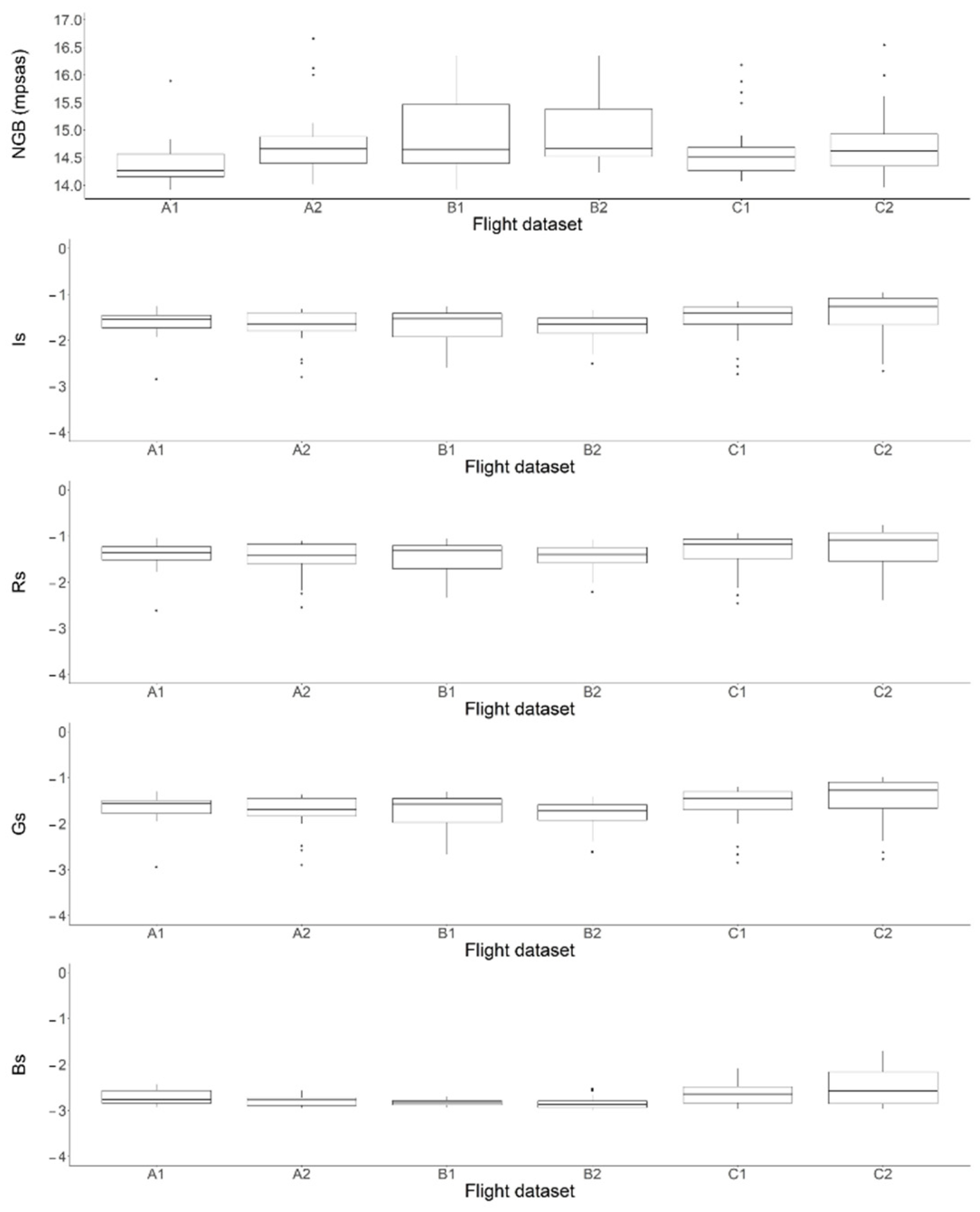
3.1. Night Ground Brightness (NGB) Measurements and Indices of Luminous Intensity

The NGB measurements taken during all the flight campaigns are presented in Figure 4. In the study area, the NGB varied between 13.9 mpsas in the brightest area and 17.3 mpsas in the darkest one. Thus, the brightest area was 21 times brighter than the darkest one. The lowest average NGB value of a flight was recorded during the 70-metre height flight (A1) in the first campaign (14.6 mpsas) (Figure 4). The average NGB values were slightly lower during flights at 70 m height (14.7 mpsas) than 100 m height (14.9 mpsas).
The values of the image indices are always negative due to the logarithm function applied to values varying between 0 and 1. The average Is varied between −1.73 and −1.65 for the flight with 1/6.25 s exposure time and increased with increasing exposure time to 0.25 for ¼ s (−1.54), and 0.42 for ½ s (−1.43) (Figure 4). The light coming from the surface was mainly composed on average by the red band (Rs = −1.41) since the lamps of the studied area were mainly amber lights, followed by the green band (Gs = −1.67), while the blue band was very low (Bs = −2.70).

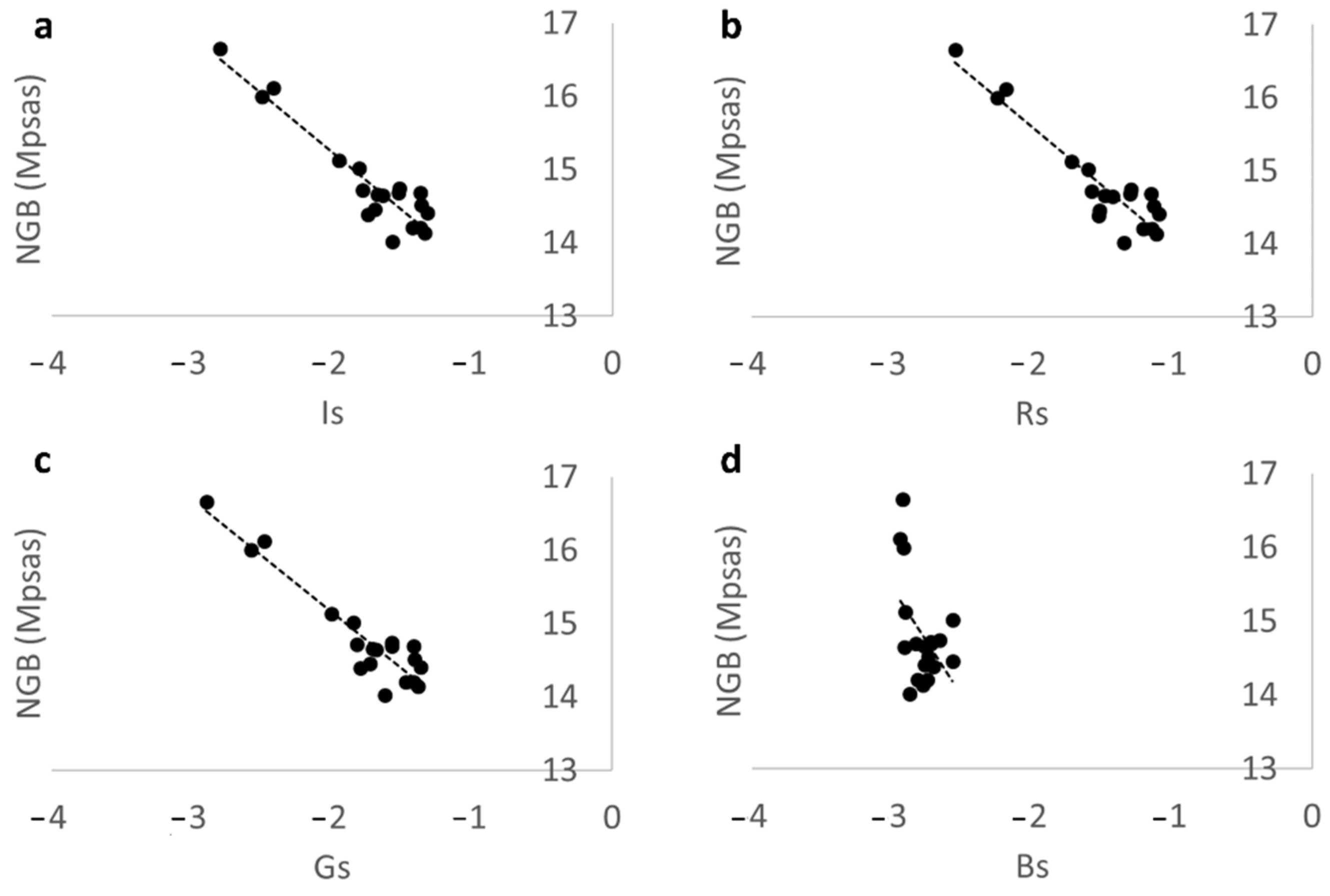
3.2. Relationship between Indices on UAV Images and SQM Measurements

Kendall rank correlation (tau) between NGB measurements and the indices was always significant with Is, Rs and Gs and never significant for Bs (Table 2). The highest value was tau = 0.58 for Rs and Gs in B1 (Table 2). Tau between NGB measurements and Is ranged between 0.49 (A1) and 0.56 (B1, A2). Tau between NGB and color bands was slightly higher for green (tau between 0.52 and 0.58 for Gs) and red color (tau between 0.42 and 0.58 for Rs) and lower for blue color (tau between −0.14 and 0.04 for Bs) (Table 2). The rank correlation with G and R color bands depends on both the spectral sensitivity of the camera, which is higher for the G component [39], and on the color of the lamps, which in our study site were mainly amber lights.
According to the coefficient of determination (R2) obtained by linear regression models between NGB and Is, Rs, Gs and Bs, the best fit was found in A2 (Table 2). Therefore, A2 was selected as a training set for computing linear regression relationships between NGB and Is and the other RGB indices. The fitted linear regression models are represented in Figure 5 and by the following formulas:
Lis = 12.805 − 1.578 ∗ Is     (N = 19, R2 = 0.87, p < 0.01)
Lrs = 12.404 − 1.599 ∗ Rs     (N = 19, R2 = 0.86, p < 0.01)
Lgs = 12.080 − 1.536 ∗ Gs     (N = 19, R2 = 0.88, p < 0.01)
Lbs = 6.683 − 2.918 ∗ Bs     (N = 19, R2 = 0.22, p < 0.05)
The best estimate of the observed NGB (Lo), using Is as a proxy, was obtained in the training set (A2) with RMSE equals 0.21 mpsas, while RMSE varied (between 0.41 and 0.46 mpsas) for the other sets (Table 3). The RMSE was slightly lower at 100 m than 70 m (0.41 mpsas in B2 vs. 0.45 and 0.46 mpsas in B1 and A1). Therefore, according to our results, the predictive capability of the linear relationship was different for different flight heights. In particular, the performance was better in both flights when the distance of the sensor from the ground was 100 m. Among the color band indices, Gs (RMSE = 0.20–0.45 mpsas) performed slightly better than Rs (RMSE = 0.22–0.49 mpsas), while Bs showed the worst performance (RMSE = 0.48–0.89 mpsas). According to ME, NGB was slightly overestimated for A1 of 0.08 mpsas for Is and underestimated (−0.08 mpsas and −0.10 mpsas, respectively, for B1 and B2). Negative average values of ME for B1 and B2 (for all indices apart from Bs) indicate that the formula calibrated on A2 tended to underestimate NGB in those datasets. This result suggests that actual environmental conditions present during flights should be taken into account.

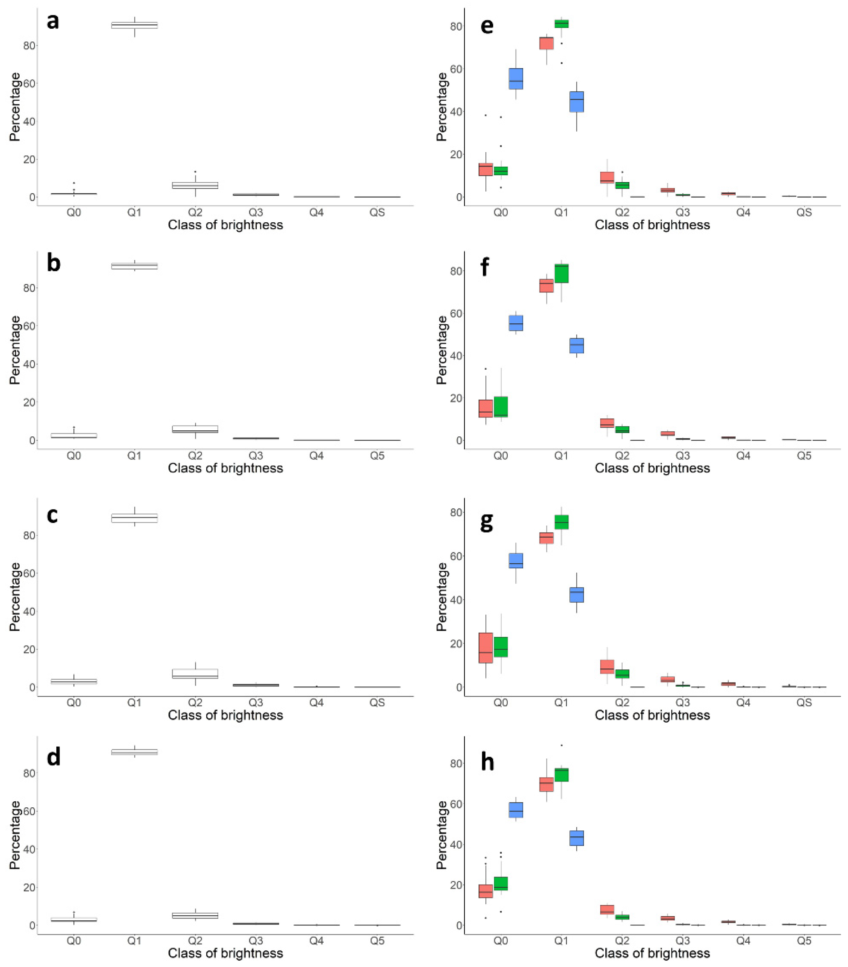
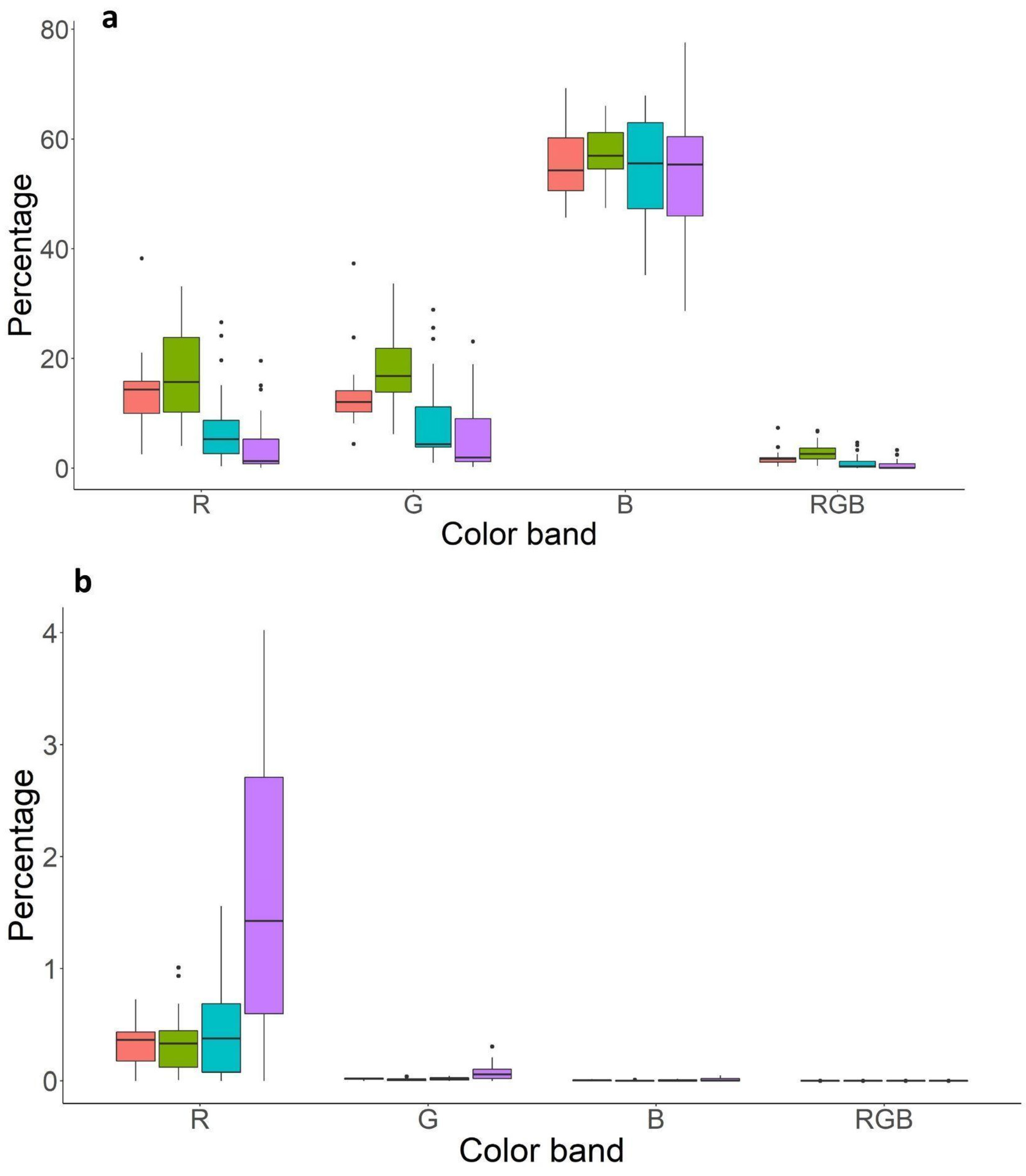
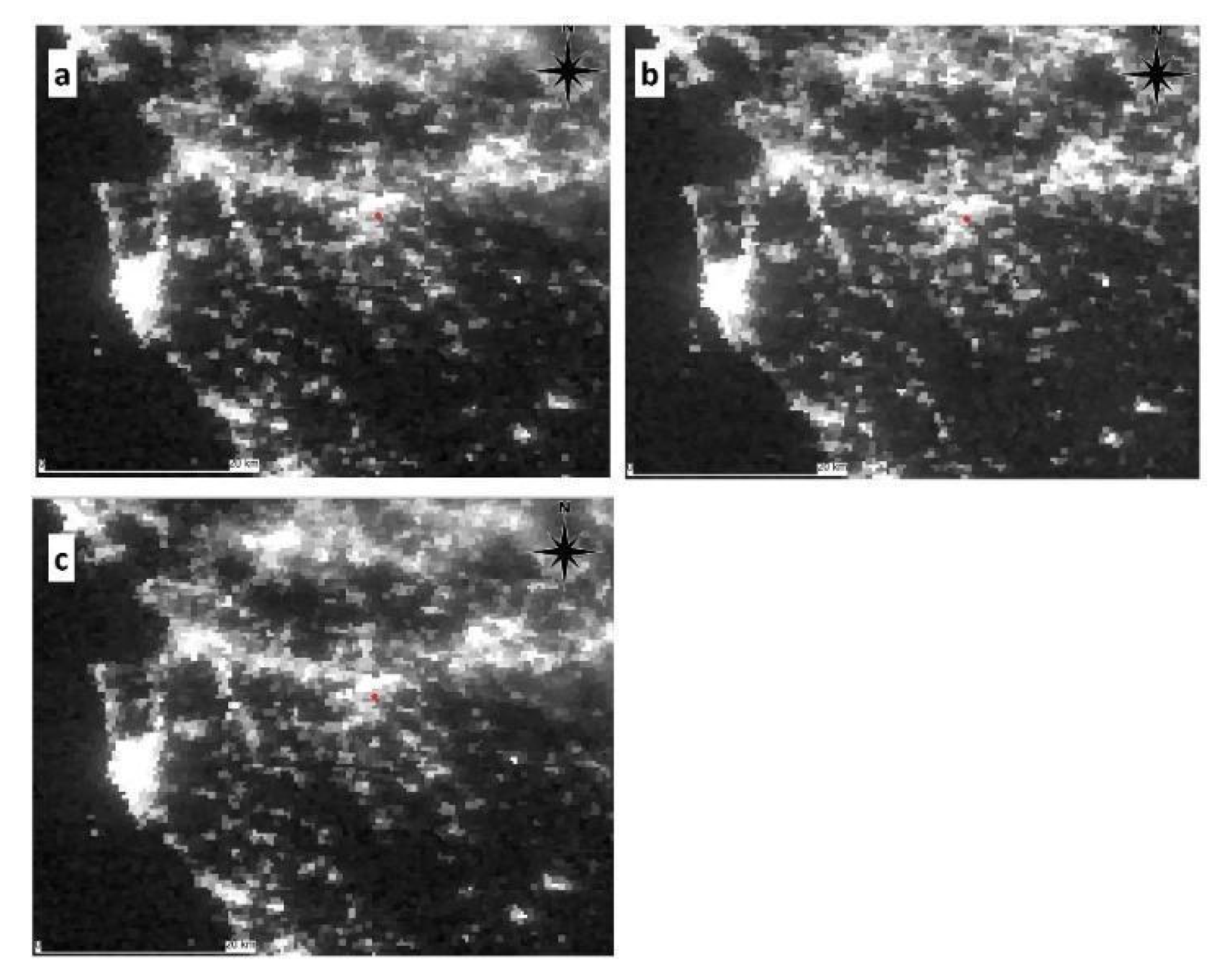
3.3. Analysis of Orthophoto in Multispectral RGB

The multispectral RGB analysis showed that both surface brightness (Q0 = 1.5%) and the color bands had a percentage of pixels below detection level varying between 10% (R and G band) to 55% for the blue band (Figure 6). This result is in contrast with another study that found no pixel below detection level [62], despite the higher dynamic range provided by RAW images used in the present study against JPEG image resolution used in Li et al. [63]. Most of the pixels are concentrated on low intensity values (>80% pixel in the first quartile) as already reported in other studies [63]. The red component had a higher percentage of pixels than the other bands for the higher classes of intensity (Q2–Q4 and QS).
We tried to reduce the Q0 percentage by acquiring orthophotos with longer time exposures (Figure 7), but the increase of saturated pixels (QS) offset the benefit of reducing Q0 pixels and weakened the relationship with NGB. In fact, the multispectral analysis conducted on the images taken at 70 m height showed a decrease of underexposed pixels and an increase of saturated ones as exposure time increased. Although saturated pixels increased by a small fraction (e.g., from 0.33% at 1/6.25 s to 1.68% at ½ s for red) as exposure time increased, the effect of increasing exposure time negatively influenced the correlation between NGB and image indices. For instance, Kendall rank correlation for Is deteriorated from −0.49 (A1 at 1/6.25 s) and −0.56 (B1 at 1/6.25 s) to −0.28 (C1 at 1/4 s) and −0.29 (C2 at ½ s).

4. Discussion and Conclusions

This study evaluated the possibility of using an unmanned aerial vehicle (UAV) equipped with an SQM and digital camera to estimate the brightness of ground surfaces. The relationship between night ground brightness measurements (NGB) taken by the SQM and RGB indices computed on RAW images taken with a digital camera were compared and a linear relationship between them was investigated.
Overall, results confirmed a highly significant Kendall rank correlation between the NGB and brightness index (Is), as well as with red and green indices (Rs, Gs), while no correlation was found with the index computed on the blue component (Bs). The correlation with the color bands depends on the type of luminaires installed in the study area. Indeed, our study area was mainly characterized by amber luminaires that have a very low blue component.
The significant level of correlation between NGB measurements taken by SQM mounted on a UAV suggests that the information, collected both at 70-m and 100-m flight altitudes, can be used to identify surfaces that are relevant sources of light pollution.
The error using image indices for the estimation of NGB was relevant. Mean error (ME) was still acceptable because it was always under or near 0.10 mpsas, while RMSE was always relevant. For instance, the NGB was estimated by Is with an RMSE between 0.21 and 0.46 mpsas. It is important to note that since the digital camera had not been calibrated, the indices derived by the images do not provide exact quantification of luminous intensity [39]. However, the original values of the data acquired by the sensor (RAW), as opposed to the compressed data (JPG), can be considered a good proxy of the brightness of each pixel. Despite this limitation, the significant correlation between the image indices and NGB indicates that the SQM can capture variations of surface brightness in the images. The lack of calibration of the digital camera versus a more accurate instrument is a limitation of this study. Improvements that can be obtained by calibrating the digital camera might be investigated in future studies.
Linear regression analysis showed that indices computed on night images (brightness index and color band indices connected to the color type of the luminaires) are a proxy of night ground brightness (NGB). Conversely, NGB is a cumulative measure of the surface brightness of the scene under the FOV of the SQM. However, it should be noted that the fitted model might depend on the characteristics of the digital camera used. Therefore, before using any digital camera, it is recommended to test the relationship between indices calculated on orthophoto and NGB by using a calibration set of images. This relationship is also affected by other factors, such as the optical properties of the atmosphere which can alter the scattering of light, and can also depend on environmental and meteorological factors other than cloudiness. Indeed, for the selection of the dates of monitoring, we selected clear and moonless sky conditions in order to work under the most homogeneous conditions possible. Since we performed this campaign during the spring season, which in Tuscany is characterized by unstable conditions (frequent cloudiness and rain events), it was very difficult to find nights that met all those criteria. Moreover, another constraint was introduced by the fact that the drone flight conditions might be affected by strong winds. In our case, we selected three dates that were characterized by similar sky conditions as can be seen from the images taken by the Day-Night Band Satellite (Figure 8).
Even though the sky conditions were similar, we observed that on 23 April 2021, both NSB and NGB values were slightly darker than the other two nights independently of the altitude. This might be due to slightly different environmental conditions, since even a low difference in atmospheric optical properties might be recorded by SQMs—which are characterized by a sensitivity that allows for distinguishing between small differences in surface brightness. The multispectral analysis highlighted the strong link between the color of the lamps and the RGB level of the images. One limitation of the multispectral analysis is due to the presence of luminaires of almost only one color type (amber) in the studied area. Further investigation on different luminaire types will be held in the near future.
Images taken at 70 m altitude with different exposure times showed that there is not an optimal exposure time able to capture the full dynamic of the scene, even using the RAW format that contained more detailed color information (65,536 levels) than JPG (256 levels). After several trials, we chose to set the camera to 400 ISO, diaphragm fn = 2.8 and exposure time 1/6.25 s, because the correlation dropped quickly for longer exposures. Using these settings, we obtained a high percentage of pixels below the detection level of our camera (Q0), in contrast with other studies that found almost no pixels below the detection level [63]. This difference might be due to camera systems that might have different characteristics and performance. In any case, we tested different exposure times to reduce the percentage of Q0 pixels, but increasing exposure time to ½ s resulted in a small reduction of the percentage of Q0 pixels and, at the same time, an increase of the percentage of the saturated pixels, which had the cumulative effect of worsening the correlation between NGB and image indices (from −0.56 to −0.28).
Our results highlight that coupling the camera with the sky quality meter can provide information on both the intensity of light pollution and the multispectral component of the luminaires in the study area. Indeed, the very high correlation between the brghtness of the portion of the image under the FOV of the SQM and NGB suggests that SQM can provide low cost and reliable information on the spatial variability of ground brightness seen from the sky. Such brightness can be considered a proxy of upward light emission towards the sky. RMSE for Is, Rs and Gs highlights a slightly better performance of the linear regression model at 100 m height, which suggests the SQM might work better at a higher distance from the ground since it has been designed to measure the brightness of diffused light from distant sources.
However, our study was performed in a small residential area with a homogeneous lighting system. Therefore, further studies in areas that include different types of lighting systems should be conducted in the future, in order to confirm and generalize these preliminary results. Other studies have used configurations that coupled camera systems mounted on UAVs with sky quality meters mounted on mobile systems (shopping carts and cars), thus comparing information taken at a certain altitude by camera with measurement of light reflected from the ground taken at approximately 1–2 m height [62,63]. Our study takes advantage of mounting the SQM on the drone just next to the camera, thus providing measurements from the same height and point of view for both systems. However, attention should be paid to the installation of this device on the drone. We set it in the rear position to avoid hindering the visibility of the camera, but this setting produced an unbalanced flight attitude, which required sufficient power from the motors to compensate for it. This is why we took the precaution of performing take-off only in manual mode. These issues also influence flight time autonomy and as a consequence the dimension of the monitored area. This limitation can be avoided by developing a more optimized support for the flight attitude in the future or by the vailability of sensors specifically designed for UAVs.
In this study, we did not perform a radiative calibration of the digital camera. Therefore, the information content of the images is dependent on the specific digital camera characteristics. This is a general issue of using digital cameras for monitoring light pollution. Indeed, the radiative calibration of some types of digital camera has already been done in previous studies; however, this procedure is also dependent on the specific digital camera. The procedure proposed in this study has the advantage of being easy to perform and could be effective in the identification of hotspots of light pollution. It also has the advantage of using low cost and commercial devices, such as the UAV and SQM used in this study, which makes this setting easily replicable in other studies. Nowadays, there are several commercial UAVs that are economical, reliable and easy to operate and these features make them suitable for these types of campaigns.
Furthermore, our results suggest that calibrated devices such as the SQM can be used to find relationships with indices derived from the orthophoto that can be applied to quantify cumulatively the luminous content of a scene. This relationship, even if it is dependent on the type of digital camera, is easy to assess and can be used to estimate hotspot areas of light pollution. For instance, the superimposition of the georeferenced measurements taken by the SQM along the drone’s route on the orthomosaic of the selected area during the same flight shows how higher values of NGB are positioned near brighter areas (Figure 9). In this figure, the obstruction effect of urban features, in this case tree canopies, is clearly visible. The bright lines are the street, while the black areas between them are caused by tree canopies that mask light emitted by luminaires. This effect can be reduced for deciduous species in winter when they are leafless [47]. Another effect that interacts with light pollution measurement is the anisotropic diffusion of light due to the presence of buildings [46]. For instance, the radiance measured from satellites depends on the viewing zenithal angle (VZA) of the sensor due to the interaction of light with buildings, especially in tall building areas [46]. The anisotropy of light in an urban environment and the monitoring of the area with different VZA is an important aspect that should be considered in future studies.
The application of UAVs, albeit still limited in this research field, has a potential for the detailed analysis of light pollution along a route over small and medium size areas such as a highway, city neighborhood or a sport facility [56,62]. It must be underlined that such monitoring should be considered as a survey to identify bright areas that indicate areas likely subjected to upward emission due to bad shielding of the luminaires or an excess of light reflected by the surfaces. This information can be used to select areas for more accurate monitoring, for which preliminary analysis is needed to assess what is affected by the limitations of this system and by the other factors of disturbance such as the partial obstruction of artificial light due to urban features that might affect the reliability of data taken from the air [46,47]. Moreover, the opportunity to monitor the first tens of meters allows an estimation of light pollution from the ground and in the portion of the atmosphere where many nocturnal species live, and this information might be interesting for studies that aim to assess the negative effect of the presence of altered night-time environments.
In conclusion, according to our study, SQM devices can be used to identify hotspot areas of light pollution by coupling them with digital cameras and possibly in the future in a standalone setting, if such devices are designed specifically to operate with UAVs. Monitoring light pollution from the air may take advantage of low cost systems that provide ready-to-use information for the selection of candidate hotspot areas of light pollution. Further investigations are needed to take into account the limitations of the specific settings used in this study, and the different illumination characteristics and other environmental factors that might affect the results—and which are complex to investigate in a real context.

Author Contributions

Conceptualization, L.M., M.P. and S.M.; methodology, L.M. and S.M.; software, M.P.; validation, L.M., S.M. and M.P.; formal analysis, L.M. and S.M. investigation, L.M., M.P. and S.M.; resources, M.P.; data curation, L.M. and M.P.; writing—original draft preparation, L.M., S.M. and M.P.; writing—review and editing, L.M., M.P. and S.M.; visualization, L.M. and M.P.; supervision, L.M.; project administration, L.M.; funding acquisition LM. All authors have read and agreed to the published version of the manuscript.

Funding

This research and the APC were funded by the BIOPROFILES “Implementation of practical environmental education to schools” project funded by the Erasmus+ Programme, grant number 2018-1-SK01-KA201-046312.

Data Availability Statement

Data supporting reported results can be found in Massetti Luciano, Paterni Marco, & Merlino Silvia. (2021). Data set—Monitoring light pollution with an unmanned aerial vehicle (Version 1) [Data set]. Zenodo. https://doi.org/10.5281/zenodo.5724019.

Conflicts of Interest

The authors declare no conflict of interest.

References

  1. Hoelker, F.; Wolter, C.; Perkin, E.K.; Tockner, K. Light pollution as a biodiversity threat. Trends Ecol. Evol. 2010, 25, 681–682. [Google Scholar] [CrossRef] [PubMed]
  2. Kyba, C.C.M.; Kuester, T.; de Miguel, A.S.; Baugh, K.; Jechow, A.; Hölker, F.; Bennie, J.; Elvidge, C.D.; Gaston, K.J.; Guanter, L. Artificially lit surface of Earth at night increasing in radiance and extent. Sci. Adv. 2017, 3, 1–9. [Google Scholar] [CrossRef] [Green Version]
  3. Kyba, C.C.M.; Hölker, F. Do artificially illuminated skies affect biodiversity in nocturnal landscapes? Landsc. Ecol. 2013, 28, 1637–1640. [Google Scholar] [CrossRef] [Green Version]
  4. Duriscoe, D.; Luginbuhl, C.; Elvidge, C. The relation of outdoor lighting characteristics to skyglow from distant cities. Light Res. Technol. 2014, 46, 35–49. [Google Scholar] [CrossRef]
  5. Longcore, T.; Rich, C. Ecological light pollution. Front. Ecol. Environ. 2004, 2, 191–198. [Google Scholar] [CrossRef]
  6. Gaston, K.J.; Bennie, J.; Davies, T.W.; Hopkins, J. The ecological impacts of nighttime light pollution: A mechanistic appraisal. Biol. Rev. 2013, 88, 912–927. [Google Scholar] [CrossRef] [PubMed]
  7. Davies, T.W.; Duffy, J.P.; Bennie, J.; Gaston, K.J. The nature, extent, and ecological implications of marine light pollution. Front. Ecol. Environ. 2014, 12, 347–355. [Google Scholar] [CrossRef] [Green Version]
  8. Gaston, K.J.; Duffy, J.P.; Bennie, J. Quantifying the erosion of natural darkness in the global protected area system: Decline of darkness within protected areas. Conserv. Biol. 2015, 29, 1132–1141. [Google Scholar] [CrossRef]
  9. Bennie, J.; Davies, T.W.; Cruse, D.; Gaston, K.J. Ecological effects of artificial light at night on wild plants. J. Ecol. 2016, 104, 611–620. [Google Scholar] [CrossRef] [Green Version]
  10. Dimitriadis, C.; Fournari-Konstantinidou, I.; Sourbèsa, L.; Koutsoubas, D.; Mazaris, A.D. Reduction of sea turtle population recruitment caused by nightlight: Evidence from the Mediterranean region. Ocean. Coast Manag. 2018, 153, 108–115. [Google Scholar] [CrossRef]
  11. Grubisic, M.; van Grunsven, R.H.A.; Kyba, C.C.M.; Manfrin, A.; Hölker, F. Insect declines and agroecosystems: Does light pollution matter?: Insect declines and agroecosystems. Ann. Appl. Biol. 2018, 173, 180–189. [Google Scholar] [CrossRef]
  12. Grubisic, M.; Haim, A.; Bhusal, P.; Dominoni, D.M.; Gabriel, K.M.A.; Jechow, A.; Kupprat, F.; Lerner, A.; Marchant, P.; Riley, W.; et al. Light pollution, circadian photoreception, and melatonin in vertebrates. Sustainability 2019, 11, 6400. [Google Scholar] [CrossRef] [Green Version]
  13. Dominoni, D.M.; Smit, J.A.H.; Visser, M.E.; Halfwerk, W. Multisensory pollution: Artificial light at night and anthropogenic noise have interactive effects on activity patterns of great tits (Parus major). Environ. Pollut. 2020, 256, 113314. [Google Scholar] [CrossRef] [PubMed]
  14. Maggi, E.; Bongiorni, L.; Fontanini, D.; Capocchi, A.; Dal Bello, M.; Giacomelli, A.; Benedetti-Cecchi, L. Artificial light at night erases positive interactions across trophic levels. Funct. Ecol. 2020, 34, 694–706. [Google Scholar] [CrossRef]
  15. Yang, Y.; Liu, Q.; Wang, T.; Pan, J. Light pollution disrupts molecular clock in avian species: A power-calibrated meta-analysis. Environ. Pollut. 2020, 265, 114206. [Google Scholar] [CrossRef] [PubMed]
  16. Cathey, A.R.; Campbell, L.E. Effectiveness of five vision-lighting sources on photoregulation of 22 species of ornamental plants. J. Am. Soc. Hortic. Sci. 1975, 100, 65–71. [Google Scholar]
  17. Ffrench-Constant, R.H.; Somers-Yeates, R.; Bennie, J.; Economou, T.; Hodgson, D.; Spalding, A.; McGregor, P.K. Light pollution is associated with earlier tree budburst across the United Kingdom. Proc. R. Soc. B 2016, 283, 20160813. [Google Scholar] [CrossRef]
  18. Škvareninová, J.; Tuhárska, M.; Škvarenina, J.; Babálová, D.; Slobodníková, L.; Slobodník, B.; Středová, H.; Minďaš, J.J. Effects of light pollution on tree phenology in the urban environment. Morav. Geogr. Rep. 2017, 25, 282–290. [Google Scholar] [CrossRef] [Green Version]
  19. Bennie, J.; Davies, T.W.; Cruse, D.; Inger, R.; Gaston, K.J. Artificial light at night causes top-down and bottom-up trophic effects on invertebrate populations. J. Appl. Ecol. 2018, 55, 2698–2706. [Google Scholar] [CrossRef]
  20. Massetti, L. Assessing the impact of street lighting on Platanus x acerifolia phenology. Urban Urban Green 2018, 34, 71–77. [Google Scholar] [CrossRef]
  21. Haim, A.; Abed, E.Z. Artificial light at night: Melatonin as a mediator between the environment and epigenome. Phil. Trans. R. Soc. B 2015, 370, 20140121. [Google Scholar] [CrossRef] [PubMed] [Green Version]
  22. Touitou, Y.; Reinberg, A.; Touitou, D. Association between light at night, melatonin secretion, sleep deprivation, and the internal clock: Health impacts and mechanisms of circadian disruption. Life Sci. 2017, 173, 94–106. [Google Scholar] [CrossRef] [PubMed]
  23. Svechkina, A.; Portnov, B.A.; Trop, T. The impact of artificial light at night on human and ecosystem health: A systematic literature review. Landsc. Ecol. 2020, 35, 1725–1742. [Google Scholar] [CrossRef]
  24. Shi, K.; Yu, B.; Huang, Y.; Hu, Y.; Yin, B.; Chen, Z.; Chen, L.; Wu, J. Evaluating the Ability of NPP-VIIRS Nighttime Light Data to Estimate the Gross Domestic Product and the Electric Power Consumption of China at Multiple Scales: A Comparison with DMSP-OLS Data. Remote Sens. 2014, 6, 1705–1724. [Google Scholar] [CrossRef] [Green Version]
  25. Katz, Y.; Levin, N. Quantifying urban light pollution—A comparison between field measurements and EROS-B imagery. Remote Sens. Environ. 2016, 177, 65–77. [Google Scholar] [CrossRef]
  26. Levin, N.; Kyba, C.C.M.; Zhang, Q.; de Miguel, A.S.; Román, M.O.; Li, X.; Portnov, B.A.; Molthan, A.L.; Jechow, A.; Miller, S.D.; et al. Remote sensing of night lights: A review and an outlook for the future. Remote Sens. Environ. 2020, 237, 111443. [Google Scholar] [CrossRef]
  27. Barentine, J.C.; Walczak, K.; Gyuk, G.; Tarr, C.; Longcore, T. A Case for a New Satellite Mission for Remote Sensing of Night Lights. Remote Sens. 2021, 13, 2294. [Google Scholar] [CrossRef]
  28. Ribas, S.J.; Figueras, F.; Paricio, S.; Canal-Domingo, R.; Torra, J. How clouds are amplifying (or not) the effects of ALAN. Int. J. Sustain. Light 2016, 35, 32–39. [Google Scholar] [CrossRef]
  29. Posch, T.; Binder, F.; Puschnig, J. Systematic measurements of the night sky brightness at 26 locations in Eastern Austria. J. Quant. Spectrosc. Radiat. Transf. 2018, 211, 144–165. [Google Scholar] [CrossRef] [Green Version]
  30. Bará, S.; Lima, R.C.; Zamorano, J. Monitoring Long-Term Trends in the Anthropogenic Night Sky Brightness. Sustainability 2019, 11, 3070. [Google Scholar] [CrossRef] [Green Version]
  31. Bertolo, A.; Binotto, R.; Ortolani, S.; Sapienza, S. Measurements of Night Sky Brightness in the Veneto Region of Italy: Sky Quality Meter Network Results and Differential Photometry by Digital Single Lens Reflex. J. Imaging 2019, 5, 56. [Google Scholar] [CrossRef] [PubMed] [Green Version]
  32. Zamorano, J.; Tapia, C.; Pascual, S.; García, C.; González, R.; González, E.; Corcho, O.; García, L.; Gallego, J.; de Miguel, A.S.; et al. Night sky brightness monitoring in Spain. In Proceedings of the Highlights on Spanish Astrophysics X. Proceedings of the XIII Scientific Meeting of the Spanish Astronomical Society, Salamanca, Spain, 16–20 July 2018; Montesinos, B., Asensio Ramos, A., Buitrago, F., Schödel, R., Villaver, E., Pérez-Hoyos, S., Ordóñez-Etxeberria, I., Eds.; pp. 599–604, ISBN 978-84-09-09331-1. [Google Scholar]
  33. Massetti, L. Drivers of artificial light at night variability in urban, rural and remote areas. J. Quant. Spectro. Radiat. Trans. 2020, 255, 107250. [Google Scholar] [CrossRef]
  34. Caruana, J.; Vella, R.; Spiteri, D.; Nolle, M.; Fenech, S.; Aquilina, N.J. A photometric mapping of the night sky brightness of the Maltese islands. J. Environ. Manag. 2020, 261, 110196. [Google Scholar] [CrossRef] [Green Version]
  35. Lampar, H.A.S.; Kocifaj, M. Urban artificial light emission function determined experimentally using night sky images. J. Quant. Spectrosc. Radiat. 2016, 181, 87–95. [Google Scholar]
  36. Jechow, A.; Kolláth, Z.; Ribas, S.J.; Spoelstra, H.; Hölker, F.; Kyba, C.C.M. Imaging and mapping the impact of clouds on skyglow with all-sky photometry. Sci. Rep. 2017, 7, 6741. [Google Scholar] [CrossRef] [PubMed]
  37. Kolláth, Z.; Dömény, A. Night sky quality monitoring in existing and planned dark sky parks by digital cameras. Int. J. Sustain. Light 2017, 19, 61–68. [Google Scholar] [CrossRef]
  38. Jechow, A.; Ribas, S.J.; Domingo, R.C.; Hölker, F.; Kolláth, Z.; Kyba, C.C.M. Tracking the dynamics of skyglow with differential photometry using a digital camera with fisheye lens. J. Quant. Spectrosc. Radiat. Transf. 2018, 209, 212–223. [Google Scholar] [CrossRef] [Green Version]
  39. Hänel, A.; Posch, T.; Ribas, S.J.; Aubé, M.; Duriscoe, D.; Jechow, A.; Kollath, Z.; Lolkema, D.E.; Moore, C.; Schmidt, N.; et al. Measuring night sky brightness: Methods and challenges. J. Quant. Spectrosc. Radiat. Transf. 2018, 205, 278–290. [Google Scholar] [CrossRef] [Green Version]
  40. De Miguel, A.S.; Aubé, M.; Zamorano, J.; Kocifaj, M.; Roby, J.; Tapia, C. Sky Quality Meter measurements in a colour-changing world. Mon. Not. R. Astron. Soc. 2017, 467, 2966–2979. [Google Scholar] [CrossRef]
  41. Puschnig, J.; Näslund, M.; Schwope, A.; Wallner, S. Correcting sky-quality-meter measurements for ageing effects using twilight as calibrator. Mon. Not. R. Astron. Soc. 2021, 502, 1095–1103. [Google Scholar] [CrossRef]
  42. Bartolomei, M.; Olivieri, L.; Bettanini, C.; Cavazzani, S.; Fiorentin, P. Verification of Angular Response of Sky Quality Meter with Quasi-Punctual Light Sources. Sensors 2021, 21, 7544. [Google Scholar] [CrossRef] [PubMed]
  43. Schmidt, W.; Spoelstra, H. Darkness Monitoring in the Netherlands 2009–2019; NachtMeetnet: Utrecht, The Netherlands, 2020. [Google Scholar]
  44. Falchi, F.; Cinzano, P.; Duriscoe, D.; Kyba, C.C.M.; Elvidge, C.D.; Baugh, K.; Portno, B.; Rybnikova, N.A.; Furgoni, R. The new world atlas of artificial night sky brightness. Sci. Adv. 2016, 2, e1600377. [Google Scholar] [CrossRef] [PubMed] [Green Version]
  45. Kyba, C.C.M.; Garz, S.; Kuechly, H.; de Miguel, A.S.; Zamorano, J.; Fischer, J.; Holker, F. High-resolution imagery of earth at night: New sources, opportunities and challenges. Remote Sens. 2015, 7, 1–23. [Google Scholar] [CrossRef] [Green Version]
  46. Li, X.; Ma, R.; Zhang, Q.; Li, D.; Liu, S.; He, T.; Zhao, L. Anisotropic characteristic of artificial light at night—systematic investigation with viirs dnb multi-temporal observations. Remote Sens. Environ. 2019, 233, 111357. [Google Scholar] [CrossRef]
  47. Li, X.J.; Duarte, F.; Ratti, C. Analyzing the obstruction effects of obstacles on light pollution caused by street lighting system in cambridge, massachusetts. Environ. Plan. B Urban Anal. City Sci. 2021, 48, 216–230. [Google Scholar] [CrossRef]
  48. Di Gennaro, S.F.; Toscano, P.; Cinat, P.; Berton, A.; Matese, A. A Low-Cost and Unsupervised Image Recognition Methodology for Yield Estimation in a Vineyard. Front. Plant Sci. 2019, 10, 559. [Google Scholar] [CrossRef] [Green Version]
  49. Dainelli, R.; Toscano, P.; Di Gennaro, S.F.; Matese, A. Recent Advances in Unmanned Aerial Vehicles Forest Remote Sensing—A Systematic Review. Part II: Research Applications. Forests 2021, 12, 397. [Google Scholar] [CrossRef]
  50. Luppichini, M.; Bini, M.; Paterni, M.; Berton, A.; Merlino, S. A New Beach Topography-Based Method for Shoreline Identification. Water 2020, 12, 3110. [Google Scholar] [CrossRef]
  51. Andriolo, U.; Gonçalves, G.; Bessa, F.; Sobral, P. Mapping marine litter on coastal dunes with unmanned aerial systems: A showcase on the Atlantic Coast. Sci. Total Environ. 2020, 736, 139632. [Google Scholar] [CrossRef]
  52. Merlino, S.; Paterni, M.; Berton, A.; Massetti, L. Unmanned Aerial Vehicles for Debris Survey in Coastal Areas: Long-Term Monitoring Programme to Study Spatial and Temporal Accumulation of the Dynamics of Beached Marine Litter. Remote Sens. 2020, 12, 1260. [Google Scholar] [CrossRef] [Green Version]
  53. Salgado-Hernanz, P.M.; Bauza, J.; Alomar, C.; Compa, M.; Romero, L.; Deudero, S. Assessment of marine litter through remote sensing: Recent approaches and future goals. Mar. Pollut. Bull. 2021, 168, 112347. [Google Scholar] [CrossRef] [PubMed]
  54. Pucino, N.; Kennedy, D.M.; Carvalho, R.C.; Allan, B.; Ierodiaconou, D. Citizen science for monitoring seasonal-scale beach erosion and behaviour with aerial drones. Sci. Rep. 2021, 11, 3935. [Google Scholar] [CrossRef] [PubMed]
  55. Merlino, S.; Paterni, M.; Locritani, M.; Andriolo, U.; Gonçalves, G.; Massetti, L. Citizen science for marine litter detection and classification on Unmanned Aerial Vehicle images. Water 2021, 13, 3349. [Google Scholar] [CrossRef]
  56. Bouroussis, C.A.; Topalis, F.V. Assessment of outdoor lighting installations and their impact on light pollution using unmanned aircraft systems-The concept of the drone-gonio-photometer. J. Quant. Spectrosc. Radiat. Transf. 2020, 253, 107155. [Google Scholar] [CrossRef]
  57. Reagan, J. Spanish Company Deploys Drones to Battle Light Pollution. 2018. Available online: https://dronelife.com/2018/02/13/spanish-company-deploys-drones-battle-lightpollution/ (accessed on 21 April 2022).
  58. Fiorentin, P.; Bettanini, C.; Bogoni, D. Calibration of an Autonomous Instrument for Monitoring Light Pollution from Drones. Sensors 2019, 23, 5091. [Google Scholar] [CrossRef] [Green Version]
  59. Guk, E.; Levin, N. Analyzing spatial variability in nighttime lights using a high spatial resolution color Jilin-1 image—Jerusalem as a case study. J. Photogramm. Remote Sens. 2020, 163, 121–136. [Google Scholar] [CrossRef]
  60. Kong, W.; Cheng, J.; Liu, X.; Zhang, F.; Fei, T. Incorporating nocturnal UAV sideview images with VIIRS data for accurate population estimation: A test at the urban administrative district scale. Int. J. Remote Sens. 2019, 40, 8528–8546. [Google Scholar] [CrossRef]
  61. Tabaka, P. Pilot Measurement of Illuminance in the Context of Light Pollution Performed with an Unmanned Aerial Vehicle. Remote Sens. 2020, 12, 2124. [Google Scholar] [CrossRef]
  62. Xu, Y.; Knudby, A.; Côté-Lussier, C. Mapping ambient light at night using field observations and high-resolution remote sensing imagery for studies of urban environments. Build. Environ. 2018, 145, 104–114. [Google Scholar] [CrossRef]
  63. Li, X.; Levin, N.; Xie, J.; Li, D. Monitoring hourly night-time light by an unmanned aerial vehicle and its implications to satellite remote sensing. Remote Sens. Environ. 2020, 247, 111942. [Google Scholar] [CrossRef]
  64. Darrodi, M.M.; Finlayson, G.; Goodman, T.; Mackiewicz, M. Reference data set for camera spectral sensitivity estimation. J. Opt. Soc. Am. A 2018, 32, 381–391. [Google Scholar] [CrossRef] [PubMed] [Green Version]
  65. Burggraaff, O.; Schmidt, N.; Zamorano, J.; Pauly, K.; Pascual, S.; Tapia, C.; Spyrakos, E.; Snik, F. Standardized spectral and radiometric calibration of consumer cameras. Optics Express 2019, 27, 19075–19101. [Google Scholar] [CrossRef] [PubMed] [Green Version]
  66. Kolláth, Z.; Cool, A.; Jechow, A.; Kolláth, K.; Száz, D.; Tong, K.-P. Introducing the dark sky unit for multi-spectral measurement of the night sky quality with commercial digital cameras. J. Quant. Spectro. Radiat. Trans. 2019, 253, 107162. [Google Scholar] [CrossRef]
  67. Leeuw, T.; Boss, E. The HydroColor app: Above water measurements of remote sensing reflectance and turbidity using a smartphone camera. Sensors 2018, 18, 256. [Google Scholar] [CrossRef] [Green Version]
  68. Kyba, C.C.M.; Ruhtz, T.; Fischer, J.; Hölker, F. Cloud Coverage Acts as an Amplifier for Ecological Light Pollution in Urban Ecosystems. PLoS ONE 2011, 6, e17307. [Google Scholar] [CrossRef] [PubMed] [Green Version]
  69. Puschnig, J.; Schwope, A.; Posch, T.; Schwarz, R. The night sky brightness at Potsdam-Babelsberg including overcast and moonlit conditions. J. Quant. Spectro. Radiat. Trans. 2014, 139, 76–81. [Google Scholar] [CrossRef] [Green Version]
  70. Cavazzani, S.; Ortolani, S.; Bertolo, A.; Binotto, R.; Fiorentin, P.; Carraro, G.; Saviane, I.; Zitelli, V. Sky Quality Meter and satellite correlation for night cloud-cover analysis at astronomical sites. Mon. Not. R. Astron. Soc. 2020, 493, 2463–2471. [Google Scholar] [CrossRef] [Green Version]
  71. Bará, S.; Rigueiro, I.; Lima, R.C. Monitoring transition: Expected night sky brightness trends in different photometric bands. J. Quant. Spectro. Radiat. Trans. 2019, 239, 106644. [Google Scholar] [CrossRef] [Green Version]
  72. Cinzano, P. Report on Sky Quality Meter, Version L. 2007. Available online: http://unihedron.com/projects/sqm-l/sqmreport2.pdf (accessed on 25 October 2021).
  73. Poynton, C. Digital Video and HD: Algorithms and Interfaces; Elsevier: Amsterdam, The Netherlands, 2012. [Google Scholar]
Figure 1. Studied area (yellow box) and flight route (dashed red line).
Remotesensing 14 02052 g001
Figure 2. Sky quality meter (SQM) mounted on the unmanned aerial vehicle (UAV).
Remotesensing 14 02052 g002
Figure 3. Point of view of the drone, sample image and projection of relative radiance (rr) as a function of the field of view, derived by [72] (red dashed line) and approximated by Equation (1) (black continuous line).
Remotesensing 14 02052 g003
Figure 4. Boxplot of NGB in magnitude/arcsec2 (mpsas) and of image indices Is, Rs, Gs and Bs for set of images taken at 1/6.25 s at 70 m (A1) and 100 m (A2) height on 3 April 2021, at 1/6.25 s and at 70 m (B1) and 100 m (B2) height on 23 April 2021 and at 70 m height and ¼ s (C1) and ½ s (C2) time exposure on 15 June 2021.
Remotesensing 14 02052 g004
Figure 5. Linear regression between NGB measurements in magnitude/arcsec2 (mpsas) and Is (a), Rs (b), Gs (c) and Bs (d) computed on RAW images of the training set A2.
Remotesensing 14 02052 g005
Figure 6. Boxplot of percentage of pixels per class of intensity: I = 0 (Q0), I = 1 (QS) or I falling in the first (Q1), the second (Q2), the third (Q3) and the fourth (Q4) quartiles for A1, A2, B1 and B2 (ad). Boxplot of percentage of pixels per class of intensity: R = 0 (Q0), R = 1 (QS) or R falling in the first (Q1) the second (Q2), the third (Q3) and the fourth (Q4) quartiles for A1, A2, B1 and B2 (red boxes in eh). Boxplot of percentage of pixels per class of intensity: G = 0 (Q0), G = 1 (QS) or G falling in the first (Q1), the second (Q2), the third (Q3) and the fourth (Q4) quartiles for A1, A2, B1 and B2 (green boxes in eh). Boxplot of percentage of pixels per class of intensity: B = 0 (Q0), B = 1 (QS) or B falling in the first (Q1), the second (Q2), the third (Q3) and the fourth (Q4) quartiles for A1, A2, B1 and B2 (blue boxes in eh).
Remotesensing 14 02052 g006
Figure 7. Boxplot of percentage of pixels per color band (R, G and B) and intensity (RGB or I) for class intensity Q0 (respectively pixels with R = 0, G = 0, B = 0 and I = 0) in the upper graphs (a) and for class intensity QS (respectively pixels with R = 1, G = 1, B = 1 and I = 1) in the lower graph (b) for the flights at 70 m and different exposure time: A1 (red) and A2 (green) at 1/6.25 s, C1 (blue) at ¼ s and C2 (violet) at ½ s.
Remotesensing 14 02052 g007
Figure 8. Satellite night view of central-west Tuscany of the three flight campaigns 3 April 2021 (a), 23 April 2021 (b) and 15 June 2021 (c). Images are provided by VIIRS Day-Night Band Satellite, white colors are the lights emitted from the Earth’s surface The study area is indicated by a red dot.
Remotesensing 14 02052 g008
Figure 9. Georeferenced night ground brightness (NGB) measured in magnitude/arcsec2 (mpsas) recorded by the UAV along the route at 70 m height on 3 April 2021 displayed upon the georeferenced night images taken by the digital camera during the same flight. Colors indicate NGB in mpsas.
Remotesensing 14 02052 g009
Table 1. Date, altitude, camera settings and number of images of each flight and night sky brightness (NSB) at the beginning and end of each flight measured in a dark location near the study area by pointing the sky quality meter to the zenith.
DatasetNightAltitude (m)Number of ImagesCamera SettingNSB (mpsas)
(Begin–End)
A13 April 20217014fn = 2.8,
exp = 1/6.25 s,
ISO = 400
19.08–19.05
A23 April 202110019fn = 2.8,
exp = 1/6.25 s,
ISO = 400
19.05–19.00
B123 April 20217023fn = 2.8,
exp = 1/6.25 s,
ISO = 400
19.09–19.11
B223 April 202110025fn = 2.8,
exp = 1/6.25 s,
ISO = 400
19.11–19.19
C115 June 20217025fn = 2.8,
exp = ¼ s,
ISO = 400
19.04–19.07
C215 June 20217028fn = 2.8,
exp = ½ s,
ISO = 400
18.99–18.91
Table 2. Kendall rank correlation (tau) and coefficient of determination according to linear regression analysis (R2) between sky quality meter (NGB) measurements and Is, Rs, Gs and Bs indices calculated respectively on RAW images taken by UAV at 70 m and 100 m above the ground. Significance levels were reported for p < 0.05 (indicated by *) and p < 0.01 (indicated by **).
IndexDateSetDistanceN. ImagestauR2
Is3 April 2021A17014−0.49 *0.76 **
Rs3 April 2021A17014−0.42 *0.72 **
Gs3 April 2021A17014−0.53 **0.77 **
Bs3 April 2021A170140.040.05
Is3 April 2021A210019−0.56 **0.87 **
Rs3 April 2021A210019−0.56 **0.86 **
Gs3 April 2021A210019−0.56 **0.88 **
Bs3 April 2021A210019−0.140.22 *
Is23 April 2021B17023−0.56 **0.57 **
Rs23 April 2021B17023−0.58 **0.57 **
Gs23 April 2021B17023−0.58 **0.58 **
Bs23 April 2021B17023−0.080.33 **
Is23 April 2021B210025−0.53 **0.53 **
Rs23 April 2021B210025−0.51 **0.5 **
Gs23 April 2021B210025−0.52 **0.55 **
Bs23 April 2021B2100250.010.03
Table 3. Mean error (ME) and root mean square error (RMSE) for the estimation of observed NGB using the fitted regression formulas for RAW images on the training set (A2, first UAV flight at 100 m height) and the three validation sets (A1 and B1, first and second flight at 70 m height and B2, the second flight at 100 m height).
ErrorSetIsRsGsBs
A10.080.110.070.00
ME (mpsas)A2 10.000.000.000.00
B1−0.08−0.08−0.090.06
B2−0.10−0.17−0.070.03
A10.460.490.450.89
RMSE (mpsas)A2 10.210.220.200.48
B10.450.450.450.57
B20.410.450.400.67
1 A2 training set.
Publisher’s Note: MDPI stays neutral with regard to jurisdictional claims in published maps and institutional affiliations.

