Communication

Soil Moisture Retrieval from the CyGNSS Data Based on a Bilinear Regression

1
School of Remote Sensing and Geomatics Engineering, Nanjing University of Information Science and Technology, Nanjing 210044, China
2
Shanghai Astronomical Observatory, Chinese Academy of Sciences, Shanghai 200030, China
3
School of Surveying and Land Information Engineering, Henan Polytechnic University, Jiaozuo 454099, China
4
Faculty of Engineering and Applied Science, Memorial University, St. John’s, NL A1B 3X5, Canada
5
School of Geographical Sciences, Nanjing University of Information Science and Technology, Nanjing 210044, China
6
Department of Surveying and Geoinformatics, Nanjing University of Posts and Telecommunications, Nanjing 210023, China
7
School of Hydrology and Water Resources, Nanjing University of Information Science and Technology, Nanjing 210044, China
8
State Key Laboratory of Hydrology Water Resources and Hydraulic Engineering, Hohai University, Nanjing 210098, China
*
Author to whom correspondence should be addressed.
Remote Sens. 2022, 14(9), 1961; https://doi.org/10.3390/rs14091961
Submission received: 15 February 2022 / Revised: 7 April 2022 / Accepted: 18 April 2022 / Published: 19 April 2022
(This article belongs to the Special Issue Recent Advances in GNSS Reflectometry)

Abstract

:
Soil moisture (SM) has normally been estimated based on a linear relationship between SM and the surface reflectivity ( Γ ) from the spaceborne Global Navigation Satellite System (GNSS)-Reflectometry, while it usually relies on inputs of SM data without considering vegetation optical depth (VOD/ τ ) effects. In this study, a new scheme is proposed for retrieving soil moisture from the Cyclone GNSS (CyGNSS) data. The variation of CyGNSS-derived Δ Γ is modeled as a function of both variations in SM and VOD ( Δ S M and Δ τ ). For retrieving SM, ancillary τ data can be obtained from the Soil Moisture Active Passive (SMAP) mission. In addition to this option, a model for simulating Δ τ is suggested as an alternative. Experimental evaluation is performed for the time span from August 2019 to July 2021. Excellent agreements between the final retrievals and referenced SMAP SM products are achieved for both training (1-year period) and test (1-year duration) sets. On the whole, overall correlation coefficients (r) of 0.97 and 0.95 and root-mean-square errors (RMSEs) of 0.024 and 0.028 cm 3 /cm 3 are obtained based on models using the SMAP and simulated Δ τ , respectively. The model without τ generates an r of 0.95 and an RMSE of 0.031 cm 3 /cm 3 . The efficiency and necessity of considering τ are thus confirmed by its enhancement based on correlation and RMSE against the one without τ , and the usefulness of approximating Δ τ by sinusoidal functions is also validated. Influences of SM statistics in terms of mean and variance on the retrieval accuracy are evaluated. This work unveils the interaction between CyGNSS data, SM, and τ and demonstrates the feasibility of integrating the Δ τ approximation function into a bilinear regression model to obtain SM results.

Graphical Abstract

1. Introduction

Monitoring and understanding the characteristics of terrestrial hydrological parameters, for example, the soil moisture (SM) distribution, are critical for the studies of climate changes and carbon cycles [1,2]. Observations from the space appear as an invaluable data source. Large-scale SM data are usually obtained by spaceborne payloads working at microwave bands, as these signals are sensitive to the dielectric property of soil that is a function of SM [3]. The spaceborne missions associated with SM measurements include Soil Moisture Active Passive (SMAP) [4], Soil Moisture and Ocean Salinity (SMOS) [5], Sentinel-1 [6], and TerraSAR-X [7], etc. However, passive microwave satellites, e.g., SMAP and SMOS, have a coarse spatial resolution of about 40 km. Furthermore, measurements from synthetic aperture radar (SAR) systems, e.g., Sentinel-1 and TerraSAR-X, are significantly affected by surface roughness and vegetation structure. Thus, it is desirable to have multiple remote sensing data sources to complement each other.
During the recent decade, the technique of Global Navigation Satellite System (GNSS)-Reflectometry (GNSS-R) has been well recognized as a useful remote sensing tool. GNSS-R utilizes the L-band signal that can efficiently propagate through the atmosphere and clouds, providing a 24-7 and all-weather surveillance [8,9]. In addition, signals at such a frequency range are recommended for SM sensing since they are more susceptible to the top-layer SM but less influenced by the surface conditions [10]. The technique of GNSS-R has been applied in, e.g., ocean wind measurement [11,12,13], altimetry [14], and ice detection [15]. With the availability of spaceborne data collected by the Cyclone GNSS (CyGNSS) constellation, retrieving SM from such dataset on a large spatial scale has become a flourishing topic [16,17,18,19,20,21,22,23,24,25,26]. Existing SM estimation approaches can be broadly divided into two categories, specifically, machine learning (ML)-, and empirical model-based methods. However, applications of ML algorithms in SM sensing (e.g., [21,22,23,26]) are generally confronted with the following challenges: (1) the dependence on a great quality of ancillary data, which may diminish the sensitivity of retrievals to CyGNSS data, (2) the difficulty in interpreting the relationships between involved physical quantities, which blurs our understanding about how GNSS-R observables respond to the target parameters, (3) the requirement of huge training data, and (4) the poor generalization capability of a trained model for other areas. Instead, the model-based inversions usually rely on less auxiliary inputs, present clearer links between the CyGNSS observables and desired SM data, and can be locally parameterized. Clarizia et al. [19] developed a trilinear regression function to interpret the association of reflectivity-vegetation-roughness for estimating SM, and Yan et al. [25] adopted a similar approach while utilizing CyGNSS-derived observables to resolve the surface roughness effect. Those two models were constructed for a quasi-global application over CyGNSS-covered areas. Chew and Small [17,18] found a strong correlation between the variations of SM ( Δ SM) and CyGNSS data and substantiated such relationship by using a linear regression. In this study, a model-based scheme that adopts a bilinear regression (BR) is proposed for SM estimation. Relative to the studies in [19,25] that employ a unified model for large areas, models in this work are parameterized in a pixel-wise manner so that each of them can be tuned according to local characteristics. The difference between this work and that in [17,18] lies in an extra consideration of the VOD effect here, which compensates for the signal attenuation by vegetation. In summary, from the authors’ best knowledge, there is no existing model-based work that aims to address the VOD effect and to localize parameters at the same time in the GNSS-R society, which is to be investigated in this article. Although the accomplished results obtained by the previous research are very satisfactory, this work is believed to better interpret the interaction between GNSS-R signals, SM, and vegetation, and consequently, to further improve the retrieval accuracy.
The remainder of this article is organized as follows: the CyGNSS and reference SMAP data are described in Section 2. The suggested SM retrieving model based on a BR algorithm is detailed in Section 3. The experimental assessment and corresponding discussions are presented in Section 4. The current work and possible future improvements are summarized in Section 5.

2. Datasets

In this section, the acquisition and preparation of CyGNSS data as well as the usage of the referenced SMAP SM and VOD data are described.

2.1. CyGNSS Remote Sensing Data

The CyGNSS Level 1 (L1) Version 3.0 datasets are adopted (available at https://podaac-tools.jpl.nasa.gov/drive/files/allData/cygnss/L1/v3.0 (accessed on 5 February 2022)), which are acquired by a constellation containing eight micro-satellites and offering GNSS-R measurements over different locations for most of the subtropics. CyGNSS is characterized by high spatial and temporal resolutions and good coverage from 38°S to 38°N. The smallest spatial resolution is approximately 3.5 km by 0.5 km and the revisit time for a 25 km-grid cell is several hours and that for a 3 km-grid cell is about 8 days [27]. The data employed here were collected over the period from August 2019 to July 2021.
The CyGNSS variables involved in this work are bistatic radar cross section (BRCS, or σ ), ancillary information about the observation and its geometry, signal-to-noise ratio (SNR), latitude and longitude of specular point (SP), distances from SP to the transmitter and receiver ( R t and R r ), etc. The data quality control scheme generally follows that in [25]. In addition, data with the quality flag “SP in the sidelobe” are rejected, for which confidence in the antenna gain is low.

2.2. Reference SMAP Products

The CyGNSS-based SM results are to be assessed with the SMAP SM data (Version 7) [28]. The spatio-temporal resolutions of the SMAP data are 36 × 36 km 2 and daily, respectively [4]. It should be noted that the SMAP (and SMOS) mission considers VOD in models and parameters that are dependent on the type of coverage. This dataset contains SM estimation, quality flag, and vegetation optical depth τ in the EASE-Grid (Version 2.0), and they are used in this work. Data with a retrieval quality flag of value 0 or 8 are retained, which indicates high-quality retrieval. SMAP products acquired between August 2019 and July 2021 are utilized.
To facilitate the experimental evaluation in a subsequent section, the CyGNSS data are spatially averaged into the EASE-Grid that is adopted by SMAP data (see also [25]). For illustration, the collocated SMAP SM/ τ and CyGNSS data averaged for the annual circle from August 2019 are presented in Figure 1 and treated as lookup tables (LUTs) for the following retrieval experiments. Land regions in white that are filtered out according to the quality flag of SMAP data are mostly covered by heavy canopy.

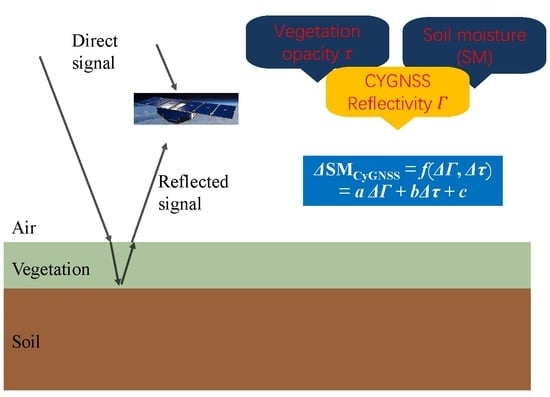
3. SM Retrieval Method

Here, the procedures of retrieving SM from CyGNSS data are detailed, consisting of computing CyGNSS observables and constructing a BR model.
In practice, CyGNSS-derived surface reflectivity Γ can be calculated using the CyGNSS BRCS σ , through assuming that coherent reflections dominate over land (see e.g., [18,19,20,21,25,29])
Γ = σ ( R t + R r ) 2 4 π ( R t R r ) 2 .
As mentioned in Section 2.1, σ , R t , and R r are respectively BRCS, and the distances from SP to the transmitter and receiver; they are available in the CyGNSS dataset.
With the premise of coherent reflections over smooth areas covered by vegetation, Γ can be modeled as [21,30]
Γ ( ϵ S , θ ) = R L ( ϵ S , θ ) 2 γ 2 exp 4 k 2 S 2 cos 2 ( θ ) ,
where R L is the surface’s Fresnel reflection coefficient, θ is the incidence angle, ϵ s denotes the dielectric constant of soil that is dependent on SM [3], transmissivity γ is the attenuation due to signal propagation through vegetation and is a function of τ , k is the signal wavenumber, and s is the surface root-mean-squared height. The exponential term depicts the effect of surface roughness. Correspondingly, the CyGNSS Γ over a smooth vegetated terrain can be associated with SM, θ , τ , and the surface roughness effect. In this present work, the model for retrieving SM is to be built based on the local fluctuations of associated variables and to be parameterized in a pixel-wise manner (see e.g., [17,18]). In consequence, the variation of surface roughness within a certain region is deemed insignificant, and thus, neglected here. In addition, the dependence of Γ on θ is corrected by following the procedure in [16,17]. Therefore, the reliance of Γ on surface roughness and θ is eliminated. In practice, ref. [16] or [17] did not compensate the effects of surface roughness nor vegetation in their retrieval models (although [16] adopted mean surface slope to resolve the surface roughness effect; such value was simply set as a fixed constant of 0.01 for all, and actually, it neglected the temporal variations of vegetation and roughness as was done in [31]). In this work, the temporal variability of surface roughness is also ignored; however, the impact of vegetation is considered through the variation of VOD. As such, a dependence between the variations in Γ , SM, and VOD ( Δ Γ , Δ S M , and Δ τ , respectively) is assumed in this study and is modeled through a BR, in the following form (as a function of SM retrieval):
Δ S M = f Δ Γ , Δ τ = a Δ log ( Γ ) + b Δ τ + c ,
where a, b, and c are coefficients to be determined. The corresponding flowchart of this proposed method is presented in Figure 2.

Modeling of Δ τ

In the case of lacking SMAP Δ τ , a model is proposed for simulating such data as an alternative. By assuming that Δ τ varies with a seasonal cycle, Δ τ m at each EASE-Grid pixel is approximated by a sinusoidal function with a fixed 12-month period (see a similar procedure in [32]), as
Δ τ m = d sin ( π 6 t + ϕ ) + g ,
where d, ϕ , and g are unknowns to be pixel-wisely determined, and t is the month index. Subsequently, a model f 1 , which is the same as Equation (3), was considered, but with Δ τ being replaced by Δ τ m , as
Δ S M = f 1 Δ Γ , Δ τ m = a 1 Δ log ( Γ ) + b 1 Δ τ m + c 1 ,
where the coefficients a 1 , b 1 , and c 1 will be determined via training.
With the determined LUTs of annual mean SM ¯ , τ ¯ , and Γ ¯ along with coefficients a, b, and c, posterior SM estimations ( SM est ) can be retrieved by inputting Γ and τ , i.e.,
SM est = a log ( Γ ) log ( Γ ¯ ) + b τ τ ¯ + c + SM ¯ .

4. Experiments and Evaluation

Here, the devised scheme for retrieving SM is performed and evaluated with SMAP data between August 2019 and July 2021. Data collected during August 2019 to July 2020 were employed as training data to derive the coefficients for Equation (3), and the rest were used as test data. In addition, a 10-fold cross-validation was adopted in the training phase to prevent overfitting.
Here, τ , SM, and Γ are aggregated on a monthly basis. It is widely accepted that monthly SM data are also critical inputs to climate change study and environment research. Although SM data with better spatio-temporal resolutions are also useful and can be achieved by CyGNSS data, the focus of this work is to prove the necessity of including VOD in the retrieval model. In addition, aggregating data monthly can secure the spatial coverage in the EASE-Grid that can facilitate the training phase (with more valid and consecutive data at each grid). More importantly, the averaging process can help improve the data quality of CyGNSS Γ in SM sensing [25]. Then, the monthly averaged τ , SM, and Γ are subtracted by their corresponding annual mean values (i.e., Figure 1) to determine the variation of each variable. The variation results are exhibited in Figure 3, Figure 4 and Figure 5 and used as the training set.
To determine the simulated Δ τ m , a least-squares fitting was performed to derive these unknowns in Equation (5) using the training data and this model was assessed with both the training and test sets. Through evaluation, an r of 0.88 and an RMSE of 0.018 between Δ τ m and Δ τ were estimated, with the density plot being displayed in Figure 6.

4.1. Determination of the Coefficients

An obvious correlation between the presented Δ log ( Γ ) and Δ S M can be well identified by visually comparing the corresponding sub-figures in Figure 4 and Figure 5. The correlation coefficient (r) between the time-series of these two variables was computed, and the outcomes are displayed in Figure 7, from which a strong and positive correlation can be obtained for most of the areas. Such correlation between Δ log ( Γ ) and Δ S M confirmed the validity of the adopted BR model. It was also noticed that Δ τ and Δ S M were related to some extent. As a result, Δ log ( Γ ) and Δ τ appeared to be positively related. However, Γ should be inversely proportional to τ , as verified subsequently based on the values of coefficients a and b in Equation (3). Through implementing a BR using the Δ S M , Δ log ( Γ ) , and Δ τ data, values of a, b, and c were determined and taken as LUTs. Regions with three or less collocated measurements were rejected in this work. Coefficients a and b illustrated in Figure 8a,b are dominated by positive values, which indicates Δ S M is generally proportional to both Δ log ( Γ ) and Δ τ ; while Δ log ( Γ ) and Δ τ are linked by the coefficient b / a , which appears mostly as negative values in Figure 8c. It can be noted that the regions with problematic coefficients coincide with a low correlation coefficient r in Figure 7, e.g., in northwest Australia. Through analyses, it was found that those places are characterized by extremely low and/or invariant SM/ τ (refer to Figure 1b,c for low SM/ τ and Figure 9 for Δ S M / Δ τ values). In addition, by referring to the land cover classification provided in the SMAP dataset (see Figure 10), these regions are typically barren, sparsely vegetated, or they have open shrublands. Furthermore, mean values of SM, VOD, and Coefficients a, b, and c ( SM ¯ , τ ¯ , a ¯ , b ¯ , and c ¯ ) for the dominant land cover type with more than 100 pixels over the globe are calculated and presented in the ascending order of SM ¯ in Table 1. It can be noticed that SM ¯ , τ ¯ , a ¯ , and c ¯ are roughly proportional to each other, while they are inversely proportional b ¯ . It can be interpreted that for regions with higher SM ¯ , τ ¯ is generally higher, and more importantly, the sensitivity of CyGNSS Γ to SM is stronger because a ¯ increases. Moreover, the changing trends of τ ¯ and a ¯ are not monotonical, respectively showing a dig and pump for cropland/natural vegetation mosaic, which proves the response of CyGNSS Γ to VOD as well. Thus, it can be summarized that CyGNSS Γ can be linked with SM and VOD, which further validates the rationality of this proposed model.

4.2. Validation and Assessment

Through examining both the 1-year long training and test data, a good agreement was found between the retrieved and reference SMs, and the density plots are shown in Figure 11. The obtained r is up to 0.98 for the training data. The use of SM ¯ facilitates the targeting of the desired value. Still, without including SM ¯ , satisfactory consistency between the estimated and reference Δ S M was reached, with an r of 0.91 and a root-mean-square error (RMSE) of 0.019 cm 3 /cm 3 . The good correlations between the derived product and the SMAP SM product can be due to their consideration of VOD. Statistical results with more details are listed in Table 2 for both training and test data. Negligible degradation of accuracy in the test dataset compared with that for the training set proved the generalization of this method. Figure 12 demonstrated the Δ S M time-series of two locations that are respectively marked by a red astride (11.51°N, 37.53°E) and a red circle (27.42°S, 119.31°E) in Figure 10. The former is characterized by good alignment between both Δ S M results and shows a clear seasonal cycle. Conversely, the latter represents a typical example with low correlation between two products. Moreover, corresponding SMs are relatively low and stable without distinct seasonal patterns. To support this argument, the impacts of mean and variance of SM on the retrieval results in terms of r were evaluated. It was confirmed that SMs with low annual average and variation were typically accompanied with higher discrepancy between two SM products and vice versa (see Figure 13).
The impact of VOD on retrieval accuracy was analyzed and no obvious evidence of varying contribution by sparse/dense vegetation was found, because the error distribution was rather uniform over different VODs. Still, the proposed method that compensates the VOD effect shows better performance than the one without, as demonstrated by Figure 14.

4.3. Sensitivity of Δ S M to Δ τ and Δ Γ

Here, the performance of the proposed model using simulated Δ τ m is assessed. Corresponding test results are shown in Table 2, and they are comparable with those of f in terms of accuracy. These results demonstrated the applicability of sinusoidal functions for simulating Δ τ m , and consequently, the successful application of Δ τ m for Δ S M inversion.
As mentioned previously, the correlation between Δ S M and Δ τ as well as Δ Γ was noticed. Here, the sensitivity of Δ S M to Δ τ and Δ Γ was investigated separately through testing two different models, f 2 and f 3 , specifically,
Δ S M = f 2 Δ Γ = a 2 Δ log ( Γ ) + b 2 ,
and
Δ S M = f 3 Δ τ m = a 3 Δ τ + b 3 ,
where a 2 , b 2 , a 3 , and b 3 are constants to be determined. After a training phase, the final appraisals are tabulated in Table 2, from which one can conclude that (1) the inclusion of both Δ τ and Δ Γ produces the best performance, even if Δ τ m instead of Δ τ is employed and (2) Δ S M is more dependent on Δ Γ than on Δ τ , which is evidenced by the better results of f 2 than f 3 . It is worth mentioning that f 2 is similar to the model adopted in [17,18], which does not compensate for the effect of τ . Our work here proved the necessity and efficiency of involving VOD in estimating SM, which is illustrated by the degraded performance (especially r for Δ S M ) of f 2 compared with both f and f 1 .

5. Conclusions

In this work, a new method is developed for retrieving soil moisture from the CyGNSS L1 data, which is fulfilled by applying a bilinear regression. The proposed BR model assumes the correlation among the variations of SM, VOD, and Γ . The performed comprehensive analyses demonstrated the validity and efficiency of this model. The agreement between the retrieved and referenced SM was satisfactory, with an overall r of up to 0.97 and an RMSE of 0.024 cm 3 /cm 3 . The results are in better accordance with the reference data where the mean and variance of SM are higher. In addition, a model was proposed as an alternative to SMAP VOD so that the posterior SM estimation could be accomplished solely from CyGNSS data. Superiority over the model without consideration of VOD illustrated the robustness of the proposed BR approach as well as the applicability of the VOD simulation scheme. Moreover, the sensitivity of the retrieval results to VOD and Γ was discussed.
In the future, this proposed method will be modified for better spatio-temporal resolutions and verified with in situ SM data. Furthermore, it is also meaningful to investigate the effect of the presence of inland water bodies. In the present work, the regions of Amazon and Congo were filtered out due to the SMAP quality flag; however, these areas are worth investigating in the future with other suitable reference data. Still, temporal changes of surface roughness and vegetation structure can influence the results and are worth considering as a future work. Moreover, different approaches have been proposed for SMAP or SMOS data to consider VOD’s effect on the SM estimates. Some approaches consider the complementarity between microwave and optical information and others are based on the simultaneous retrieval of SM and VOD [33], which is worth investigating and expanding to the GNSS-R technique in the future.

Author Contributions

Conceptualization, methodology, software, S.C., Q.Y.; validation, Q.Y., S.C., S.J., W.H.; writing—original draft preparation, S.C., Q.Y.; writing—review and editing, Q.C., S.L., Y.J., and T.C.; visualization, Q.Y.; supervision, S.J.; funding acquisition, Q.Y., S.C. All authors have read and agreed to the published version of the manuscript.

Funding

This research was funded by (1) the National Natural Science Foundation of China (42001362), (2) Research Start-up Fund of NUIST (2020R078), (3) Jiangsu Planned Projects for Postdoctoral Research Funds (2021K427C) to Qingyun Yan, and the Belt and Road Special Foundation of the State Key Laboratory of Hydrology-Water Resources and Hydraulic Engineering (Grant No. 2020491211) and the Natural Science Foundation of the Jiangsu Higher Education Institutions of China (No. 21KJB570012) to Qing Cao.

Data Availability Statement

Not applicable.

Acknowledgments

The authors are grateful to NASA EOSDIS Physical Oceanography Distributed Active Archive Center (DAAC), Jet Propulsion Laboratory, Pasadena, CA, USA, for making the CyGNSS data available, at https://www.esrl.noaa.gov/psd/ (accessed on 5 February 2022).

Conflicts of Interest

The authors declare no conflict of interest.

Abbreviations

The following abbreviations are used in this manuscript:
SMSoil Moisture
GNSSGlobal Navigation Satellite System
VODVegetation Optical Depth
CyGNSSCyclone GNSS
SMAPSoil Moisture Active Passive
RMSEsRoot-Mean-Square Errors
SMOSSoil Moisture and Ocean Salinity
GNSS-RGlobal Navigation Satellite System-Reflectometry
MLMachine Learning
BRBilinear Regression
BRCSBistatic Radar Cross Section
SNRSignal-To-Noise Ratio
SPSpecular Point
LUTsLookup Tables

References

  1. Bennett, A.C.; Penman, T.D.; Arndt, S.K.; Roxburgh, S.H.; Bennett, L.T. Climate more important than soils for predicting forest biomass at the continental scale. Ecography 2020, 43, 1692–1705. [Google Scholar] [CrossRef]
  2. Dobriyal, P.; Qureshi, A.; Badola, R.; Hussain, S.A. A review of the methods available for estimating soil moisture and its implications for water resource management. J. Hydrol. 2012, 458–459, 110–117. [Google Scholar] [CrossRef]
  3. Dobson, M.C.; Ulaby, F.T.; Hallikainen, M.T.; El-Rayes, M.A. Microwave dielectric behavior of wet soil-Part II: Dielectric mixing models. IEEE Trans. Geosci. Remote Sens. 1985, GE-23, 35–46. [Google Scholar] [CrossRef]
  4. Entekhabi, D.; Njoku, E.G.; O’Neill, P.E.; Kellogg, K.H.; Crow, W.T.; Edelstein, W.N.; Entin, J.K.; Goodman, S.D.; Jackson, T.J.; Johnson, J.; et al. The soil moisture active passive (SMAP) mission. Proc. IEEE 2010, 98, 704–716. [Google Scholar] [CrossRef]
  5. Kerr, Y.H.; Waldteufel, P.; Wigneron, J.P.; Martinuzzi, J.M.; Font, J.; Berger, M. Soil moisture retrieval from space: The Soil Moisture and Ocean Salinity (SMOS) mission. IEEE Trans. Geosci. Remote Sens. 2001, 39, 1729–1735. [Google Scholar] [CrossRef]
  6. Paloscia, S.; Pettinato, S.; Santi, E.; Notarnicola, C.; Pasolli, L.; Reppucci, A. Soil moisture mapping using Sentinel-1 images: Algorithm and preliminary validation. Remote Sens. Environ. 2013, 134, 234–248. [Google Scholar] [CrossRef]
  7. Aubert, M.; Baghdadi, N.; Zribi, M.; Douaoui, A.; Loumagne, C.; Baup, F.; El Hajj, M.; Garrigues, S. Analysis of TerraSAR-X data sensitivity to bare soil moisture, roughness, composition and soil crust. Remote Sens. Environ. 2011, 115, 1801–1810. [Google Scholar] [CrossRef] [Green Version]
  8. Jin, S.; Komjathy, A. GNSS reflectometry and remote sensing: New objectives and results. Adv. Sp. Res. 2010, 46, 111–117. [Google Scholar] [CrossRef] [Green Version]
  9. Jin, S.; Feng, G.; Gleason, S. Remote sensing using GNSS signals: Current status and future directions. Adv. Sp. Res. 2011, 47, 1645–1653. [Google Scholar] [CrossRef]
  10. De Roo, R.D.; Ulaby, F.T. Bistatic specular scattering from rough dielectric surfaces. IEEE Trans. Antennas Propag. 1994, 42, 220–231. [Google Scholar] [CrossRef]
  11. Clarizia, M.P.; Ruf, C.S.; Jales, P.; Gommenginger, C. Spaceborne GNSS-R minimum variance wind speed estimator. IEEE Trans. Geosci. Remote Sens. 2014, 52, 6829–6843. [Google Scholar] [CrossRef]
  12. Foti, G.; Gommenginger, C.; Jales, P.; Unwin, M.; Shaw, A.; Robertson, C.; Roselló, J. Spaceborne GNSS reflectometry for ocean winds: First results from the UK TechDemoSat-1 mission. Geophys. Res. Lett. 2015, 42, 5435–5441. [Google Scholar] [CrossRef] [Green Version]
  13. Liu, Y.; Collett, I.; Morton, Y.J. Application of neural network to GNSS-R wind speed retrieval. IEEE Trans. Geosci. Remote Sens. 2019, 57, 9756–9766. [Google Scholar] [CrossRef]
  14. Cardellach, E.; Rius, A.; Martin-Neira, M.; Fabra, F.; Nogues-Correig, O.; Ribo, S.; Kainulainen, J.; Camps, A.; D’Addio, S. Consolidating the precision of interferometric GNSS-R ocean altimetry using airborne experimental data. IEEE Trans. Geosci. Remote Sens. 2014, 52, 4992–5004. [Google Scholar] [CrossRef]
  15. Yan, Q.; Huang, W. Spaceborne GNSS-R sea ice detection using delay-Doppler maps: First results from the U.K. TechDemoSat-1 mission. IEEE J. Sel. Top. Appl. Earth Obs. Remote Sens. 2016, 9, 4795–4801. [Google Scholar] [CrossRef]
  16. Al-Khaldi, M.M.; Johnson, J.T.; O’Brien, A.J.; Balenzano, A.; Mattia, F. Time-series retrieval of soil moisture using CYGNSS. IEEE Trans. Geosci. Remote Sens. 2019, 57, 4322–4331. [Google Scholar] [CrossRef]
  17. Chew, C.; Small, E. Description of the UCAR/CU soil moisture product. Remote Sens. 2020, 12, 1558. [Google Scholar] [CrossRef]
  18. Chew, C.C.; Small, E.E. Soil moisture sensing using spaceborne GNSS reflections: Comparison of CYGNSS reflectivity to SMAP soil moisture. Geophys. Res. Lett. 2018, 45, 4049–4057. [Google Scholar] [CrossRef] [Green Version]
  19. Clarizia, M.P.; Pierdicca, N.; Costantini, F.; Floury, N. Analysis of CYGNSS data for soil moisture retrieval. IEEE J. Sel. Top. Appl. Earth Obs. Remote Sens. 2019, 12, 2227–2235. [Google Scholar] [CrossRef]
  20. Dong, Z.; Jin, S. Evaluation of the land GNSS-Reflected DDM coherence on soil moisture estimation from CYGNSS data. Remote Sens. 2021, 13, 570. [Google Scholar] [CrossRef]
  21. Eroglu, O.; Kurum, M.; Boyd, D.; Gurbuz, A.C. High spatio-temporal resolution CYGNSS soil moisture estimates using artificial neural networks. Remote Sens. 2019, 11, 2272. [Google Scholar] [CrossRef] [Green Version]
  22. Santi, E.; Pettinato, S.; Paloscia, S.; Clarizia, M.P.; Dente, L.; Guerriero, L.; Comite, D.; Pierdicca, N. Soil moisture and forest biomass retrieval on a global scale by using CyGNSS data and artificial neural networks. In Proceedings of the IGARSS 2020—2020 IEEE International Geoscience and Remote Sensing Symposium, Waikoloa, HI, USA, 26 September–2 October 2020; pp. 2905–5907. [Google Scholar]
  23. Senyurek, V.; Lei, F.; Boyd, D.; Gurbuz, A.C.; Kurum, M.; Moorhead, R. Evaluations of machine learning-based CYGNSS soil moisture estimates against SMAP observations. Remote Sens. 2020, 12, 3503. [Google Scholar] [CrossRef]
  24. Yan, Q.; Gong, S.; Jin, S.; Huang, W.; Zhang, C. Near real-time soil moisture in China retrieved from CyGNSS reflectivity. IEEE Geosci. Remote Sens. Lett. 2022, 19, 1–5. [Google Scholar] [CrossRef]
  25. Yan, Q.; Huang, W.; Jin, S.; Jia, Y. Pan-tropical soil moisture mapping based on a three-layer model from CYGNSS GNSS-R data. Remote Sens. Environ. 2020, 247, 111947. [Google Scholar] [CrossRef]
  26. Yang, T.; Wan, W.; Sun, Z.; Liu, B.; Li, S.; Chen, X. Comprehensive evaluation of using TechDemoSat-1 and CYGNSS data to estimate soil moisture over mainland China. Remote Sens. 2020, 12, 1699. [Google Scholar] [CrossRef]
  27. Chew, C. Spatial interpolation based on previously-observed behavior: A framework for interpolating spaceborne GNSS-R data from CYGNSS. J. Spat. Sci. 2021. [Google Scholar] [CrossRef]
  28. O’Neill, P.E.; Chan, S.; Njoku, E.G.; Jackson, T.; Bindlish, R. SMAP L3 Radiometer Global Daily 36 km EASE-Grid Soil Moisture; Version 7; National Snow and Ice Data Center: Boulder, CO, USA, 2020. [Google Scholar]
  29. Carreno-Luengo, H.; Camps, A.; Querol, J.; Forte, G. First results of a GNSS-R experiment from a stratospheric balloon over boreal forests. IEEE Trans. Geosci. Remote Sens. 2016, 54, 2652–2663. [Google Scholar] [CrossRef] [Green Version]
  30. Choudhury, B.J.; Schmugge, T.J.; Chang, A.; Newton, R.W. Effect of surface roughness on the microwave emission from soils. J. Geophys. Res. 1979, 89, 5699–5706. [Google Scholar] [CrossRef]
  31. Balenzano, A.; Mattia, F.; Satalino, G.; Davidson, M.W. Dense temporal series of C- and L-band SAR data for soil moisture retrieval over Agricultural Crops. IEEE J. Sel. Top. Appl. Earth Obs. Remote Sens. 2011, 4, 439–450. [Google Scholar] [CrossRef]
  32. Wagner, W.; Lemoine, G.; Borgeaud, M.; Rott, H. A study of vegetation cover effects on ers scatterometer data. IEEE Trans. Geosci. Remote Sens. 1999, 37, 938–948. [Google Scholar] [CrossRef]
  33. Wigneron, J.P.; Jackson, T.J.; O’Neill, P.; De Lannoy, G.; de Rosnay, P.; Walker, J.P.; Ferrazzoli, P.; Mironov, V.; Bircher, S.; Grant, J.P.; et al. Modelling the passive microwave signature from land surfaces: A review of recent results and application to the L-band SMOS & SMAP soil moisture retrieval algorithms. Remote Sens. Environ. 2017, 192, 238–262. [Google Scholar] [CrossRef]
Figure 1. Annual means of: (a) SMAP SM and (b) τ , and (c) CyGNSS Γ in log-scale.
Remotesensing 14 01961 g001aRemotesensing 14 01961 g001b
Figure 2. Flowchart of the proposed method.
Remotesensing 14 01961 g002
Figure 3. Monthly SMAP VOD variability.
Remotesensing 14 01961 g003
Figure 4. Monthly SMAP SM distribution.
Remotesensing 14 01961 g004
Figure 5. Monthly Γ CyGNSS distribution.
Remotesensing 14 01961 g005
Figure 6. Comparison of the SMAP and modeled Δ τ m .
Remotesensing 14 01961 g006
Figure 7. Correlation coefficient between Δ log ( Γ ) and Δ S M .
Remotesensing 14 01961 g007
Figure 8. Determined coefficients for Equation (3): (a) a, (b) b, and (c) b / a .
Remotesensing 14 01961 g008
Figure 9. Annual mean of: (a) | Δ S M | and (b) | Δ τ | .
Remotesensing 14 01961 g009
Figure 10. Land type data. Two separate locations that are respectively marked by a red astride (11.51°N, 37.53°E) and a red circle (27.42°S, 119.31°E) are dominated by different land types for which the retrieval performance varies.
Remotesensing 14 01961 g010
Figure 11. Density plot comparing the retrieved and SMAP SMs: (a) Training and (b) test data.
Remotesensing 14 01961 g011
Figure 12. Time-series of retrieved and referenced Δ S M at: (a) (11.51°N, 37.53°E) (East Africa, marked by astride) and (27.42°S, 119.31°E) (West Australia, represented by circle) and (b) zoomed in for West Australia. The corresponding locations are also labeled in Figure 10.
Remotesensing 14 01961 g012
Figure 13. Effects of SM statistics (a): variance and (b) mean on consistency between the retrieved and reference SMs.
Remotesensing 14 01961 g013aRemotesensing 14 01961 g013b
Figure 14. Density plot showing retrieval errors with (a) and without (b) considering VOD in the retrieval model.
Remotesensing 14 01961 g014
Table 1. Averages of coefficients, SM and VOD.
Land Type SM ¯ (cm 3 /cm 3 ) τ ¯ a ¯ b ¯ c ¯
Barren or Sparsely Vegetated0.05940.00100.024848.1977−0.0002
Open Shrublands0.08730.06090.05891.91560.0015
Grasslands0.14870.12110.08120.70780.0039
Savannas0.15840.34540.07850.73350.0067
Cropland/Natural Vegetation Mosaic0.20010.27360.12250.61060.0074
Woody Savannas0.23290.49120.07101.04430.0076
Table 2. Accuracy of SM retrieval (RMSE in cm 3 /cm 3 ).
Expression a Δ log ( Γ ) + b Δ τ + c a 1 Δ log ( Γ ) + b 1 Δ τ m + c 1 a 2 Δ log ( Γ ) + b 2 a 3 Δ τ + b 3
Category Measure f f 1 f 2 f 3
Trainingr (SM)0.980.970.960.95
r ( Δ S M )0.910.900.810.79
RMSE0.0190.0220.0270.028
Testr (SM)0.950.930.930.91
r ( Δ S M )0.810.800.720.62
RMSE0.0290.0340.0350.037
Overallr (SM)0.970.950.950.94
r ( Δ S M )0.860.860.770.71
RMSE0.0240.0280.0310.033
Publisher’s Note: MDPI stays neutral with regard to jurisdictional claims in published maps and institutional affiliations.

