Article

Drone-Borne Ground-Penetrating Radar for Snow Cover Mapping

Department of Environment, Land and Infrastructure Engineering, Politecnico di Torino, Corso Duca degli Abruzzi 24, 10129 Torino, Italy
*
Author to whom correspondence should be addressed.
Remote Sens. 2022, 14(7), 1763; https://doi.org/10.3390/rs14071763
Submission received: 31 January 2022 / Revised: 21 March 2022 / Accepted: 4 April 2022 / Published: 6 April 2022
(This article belongs to the Special Issue Emerging Remote Sensing Techniques for Monitoring Glaciers and Snow)

Abstract

:
Ground-penetrating radar (GPR) is one of the most commonly used instruments to map the Snow Water Equivalent (SWE) in mountainous regions. However, some areas may be difficult or dangerous to access; besides, some surveys can be quite time-consuming. We test a new system to fulfill the need to speed up the acquisition process for the analysis of the SWE and to access remote or dangerous areas. A GPR antenna (900 MHz) is mounted on a drone prototype designed to carry heavy instruments, fly safely at high altitudes, and avoid interference of the GPR signal. A survey of two test sites of the Alpine region during winter 2020–2021 is presented, to check the prototype performance for mapping the snow thickness at the catchment scale. We process the data according to a standard flow-chart of radar processing and we pick both the travel times of the air–snow interface and the snow–ground interface to compute the travel time difference and to estimate the snow depth. The calibration of the radar snow depth is performed by comparing the radar travel times with snow depth measurements at preselected stations. The main results show fairly good reliability and performance in terms of data quality, accuracy, and spatial resolution in snow depth monitoring. We tested the device in the condition of low snow density (<200 kg/m3) and this limits the detectability of the air–snow interface. This is mainly caused by low values of the electrical permittivity of the dry soft snow, providing a weak reflectivity of the snow surface. To overcome this critical aspect, we use the data of the rangefinder to properly detect the travel time of the snow–air interface. This sensor is already installed in our prototype and in most commercial drones for flight purposes. Based on our experience with the prototype, various improvement strategies and limitations of drone-borne GPR acquisition are discussed. In conclusion, the drone technology is found to be ready to support GPR-based snow depth mapping applications at high altitudes, provided that the operators acquire adequate knowledge of the devices, in order to effectively build, tune, use and maintain a reliable acquisition system.

1. Introduction

The ground-penetrating radar (GPR) is one of the most common geophysical techniques in alpine environments, as it is frequently used to survey glaciers, snow cover depth, to detect permafrost, and more generally to survey the internal morphology of debris and sediments [1,2,3]. Measuring the snow thickness, along with its density, is a common method to estimate the Snow Water Equivalent (SWE), commonly referred to as the amount of water (in the form of snow) collected by a catchment basin during the winter. The performance and the reliability of ground-based GPR to survey, at basin-catchment scale, the snow cover is well documented by several authors. Godio and Rege [4] validated the use of GPR at high altitudes to map the snow cover and the average density of snowpack. They also demonstrated the reliability of GPR in detecting snow cover up to a depth of 6–7 m with high accuracy and resolution [5]. Thanks to the capability of estimating both the snow depth and the density, GPR offers a complete and valid tool to estimate the snow thickness and therefore the SWE of catchment basins.
However, mountainous areas are not easily accessible, due to steep slopes, snow, ice, and crevasses. Therefore, the use of flying vehicles, both manned and unmanned, may overcome those difficulties in remote areas. While the use of aerial vehicles in geomatics is consolidated [6], airborne geophysical applications have been only recently developed [7,8,9,10,11,12,13]. Merz et al. highlighted the advantages of quickly exploring remote rock glaciers and rugged mountainous terrains without ground-based geophysical equipment [14]. They carried out helicopter GPR surveys on Alpine glaciers and found good reliability up to a flight height of 20 m. The study produced a 3D model of a thin-skinned rock glacier, able to display the occurrence and location of fracturing and deformation. Other authors have finally consolidated the use of helicopter-borne GPR surveys for regional-scale surveys of glacier ice thickness [15].
Such a technology suffers from greater signal attenuation compared to ground-coupled surveys. The main reasons are the divergence of the signal due to the antenna elevation [14], and the partial reflection at the air–ground (or air–ice, or air–snow) interface. Besides, knowledge of advanced processing techniques may be required to deal with the electromagnetic noise induced by the helicopter and by other sources of uncertainty such as the oscillation of the vehicle [16]. Helicopter-borne surveys are also expensive, and they are more suitable and cost-effective for regional-scale assessments, for instance when multiple glaciers are supposed to be covered during a single flight.
In small-scale surveys, some limitations are expected to be overcome by installing GPR antennas on smaller, cheaper, and more controllable airborne vehicles: the quadcopter, hexacopter, or octocopter drones [17]. In such a frame, a comparative study on ground-borne vs. drone-borne GPR was presented by Cabrera and Bekic (2018) [18]. The study pointed out that the resolving power of most GPR antennas is greatly affected by flight altitude. The drones, compared to the helicopter, can enjoy a much lower flight altitude, down to about 1 m according to our experience. The application of drone-borne GPR to investigate glacier environments is a novelty in the literature and has only been addressed by a few studies, such as Jenssen et al. (2018, 2020) [19,20]. Those works focus on the development of an ultrawideband radar antenna, operating in a frequency band between 0.95 to 6 GHz, which can be mounted effectively on an octocopter drone. The high-frequency range allowed the researchers to investigate the properties of the snow cover in arctic areas, its stratifications, and its depth. The coupling between the GPR antenna and the drone required accurate design choices to avoid interferences in the radar signal due to the presence of the drone itself, its movement, and the propellers’ rotation.
The goal of this study is to test the capabilities of a commercial radar antenna mounted on a specifically designed quadcopter drone to survey the snow-cover thickness in high-altitude alpine environments. We have designed and developed a customized drone to host a commercial radar system. For this application, a 900 MHz antenna was mounted on the drone. Some preliminary tests have been conducted at low altitude test sites, to optimize the flight procedure, test the flight-control devices, and analyze the effects of the load on the stability of the drone.
Two test sites were selected at about 2150–2200 m above sea level (a.s.l.) and the surveys were performed during the winter of 2020–2021. The first experiment was conducted at the remote basin of Cheneil, Valle d’Aosta, Italy, an area of great importance for the valley since it hosts the main sources of water that feed the local aqueduct. The drone-borne acquisitions were calibrated and compared to ground-coupled GPR acquisitions and manual snow-depth measurements. A second test was performed at the Gressoney site, also located in Valle d’Aosta, Italy, to evaluate the reliability of the air–snow pickings, sometimes uncertain in the first test site. During the second survey, we compared the GPR air–snow picking to the data collected by the laser rangefinder, a sensor already part of the drone’s setup. In both cases presented in this paper, the surveys were performed on uncontaminated snow.

2. Materials and Methods

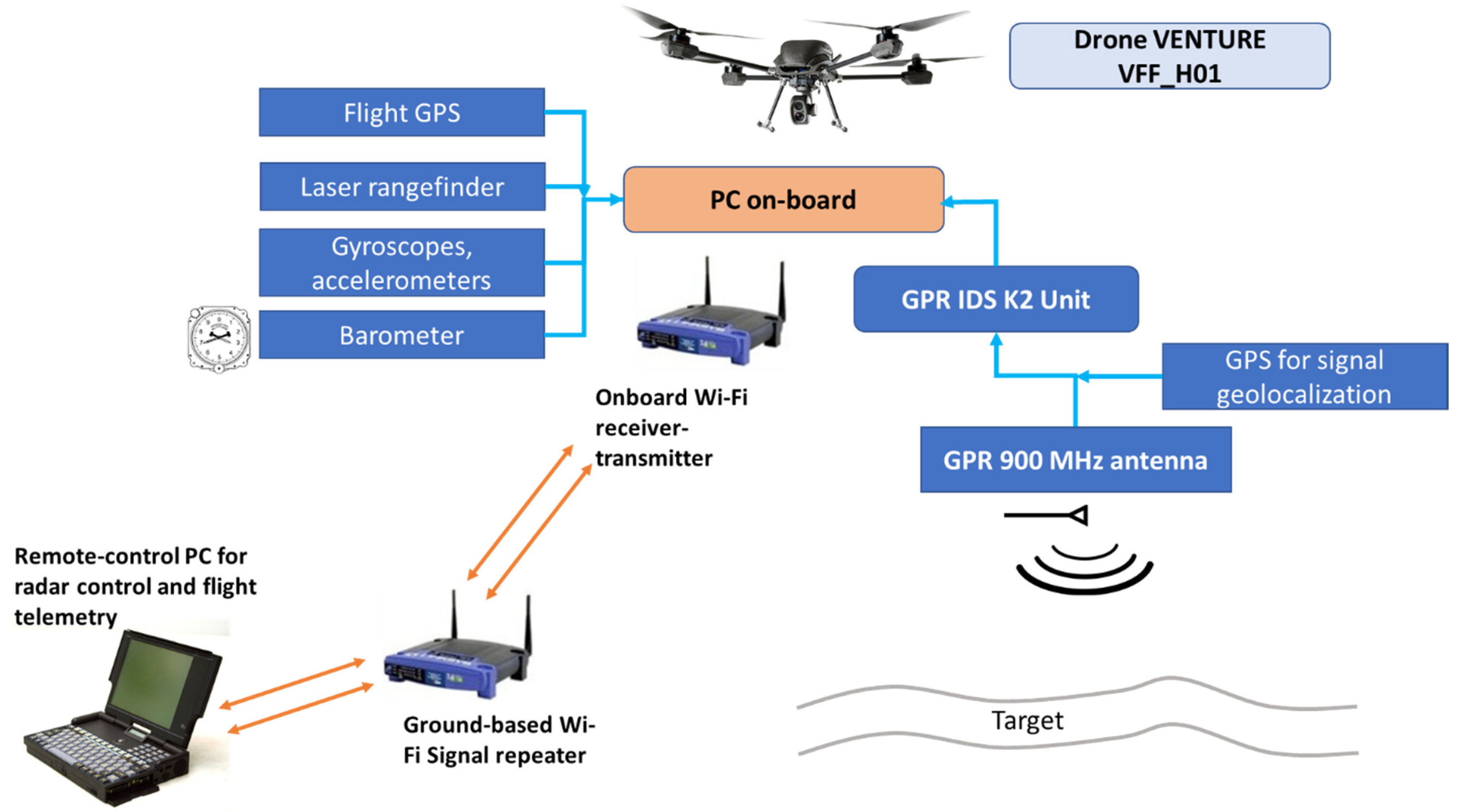
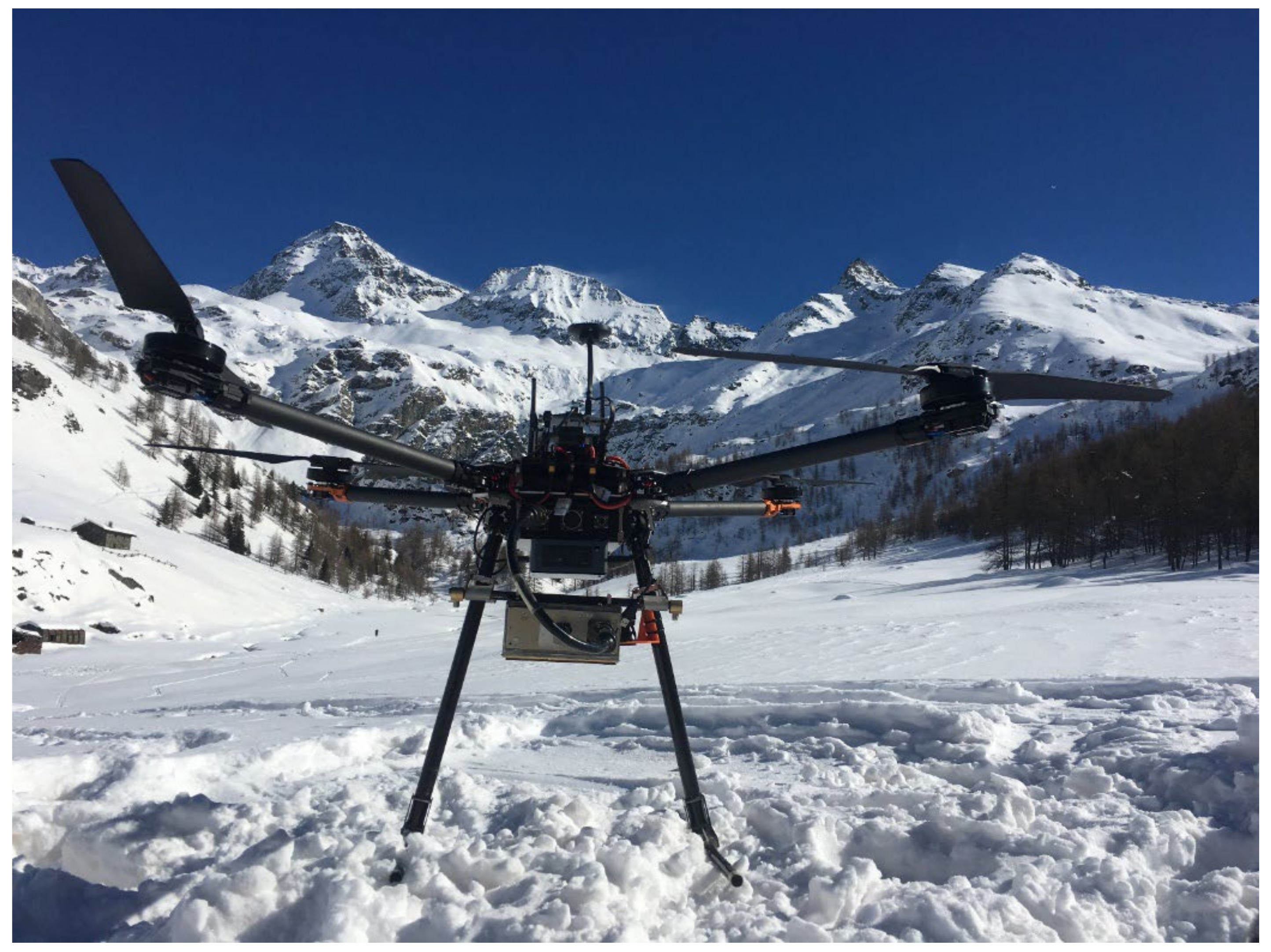
2.1. Drone Coupled with GPR Antenna

The drone developed for this research is a prototype based on the Venture VFF_H01 model, with a size of about 80 cm (height) × 2 m (width). It is bulky enough to sustain the weight of a GPR antenna and its related acquisition equipment. The GPR system is situated in the lower part of the drone structure, under the propellers, the mainboard, and the sensors of the vehicle. The devices for controlling the flight are situated at the top, as shown in the scheme and the picture (Figure 1 and Figure 2). The overall weight of the drone has been limited to 11.5 kg.
The drone is equipped with a 2-channel GPR acquisition unit and a 900 MHz antenna An onboard mini-PC allows the real-time control of the GPR acquisition system through Wi-Fi. It also controls the drone autopilot (Pixhawk 2), via “Mavlink” connection through Mission Planner software [21]. This allows the operator to check the telemetry (speed, altitude, remaining battery, etc.) in real-time, and to plan a mission with automatic flight mode. A second personal computer is the remote control of the onboard PC via LAN and TeamViewer software [22] and is handled by an operator at the base station. A router acts as a Wi-Fi signal bridge, creating the local area network needed by the PCs to communicate with each other. The frequency band used is 5 GHz. The 2.4 GHz band was not used to avoid interference with the radio controller.
The main flight control devices that compose the electronics of the drone are controlled by a Pixhawk autopilot, representing the central processing unit of the drone. It accesses and elaborates the data from various sources: the barometric sensor and the laser rangefinder for calculating the flight altitude, the gyroscopes, 3-axes accelerometers, and the GPS module for defining pitch, roll and yaw and adjusting the best flight trajectory. It receives inputs from the onboard PC, especially regarding the flight parameters, and from the radio remote control held by the pilot.
The structure of the drone is designed to allow flight at high altitudes, e.g., thanks to long propellers (wingspan = 780 mm). Where possible, such as in the propellers and the lower part of the drone, carbon fiber parts are dropped in favor of high-quality plastics to reduce radar-wave absorption by carbon fiber [23]. We observed more noise when a GPR antenna is mounted on not-specifically designed drones, as in some of our (unpublished) tests with commercial drones.
The main technical specifications of our prototype are described in Table 1.

2.2. GPR Data Processing and Data Information

The raw GPR data are postprocessed using Reflexw software [24]. First, a filter for background removal is applied. Each radargram is subtracted from an “average radargram” built up from selected radargrams in which no reflection is evident or expected. Then, the low frequencies due to instrumental electromagnetic disturbances are cut: each radargram is subtracted from its moving average (“dewow”). After a second low-pass filter, two different gain functions are applied, intrinsic attenuation recovery and geometric dispersion recovery (“divergence compensation”). In the end, stacking of traces is performed to improve the signal-to-noise ratio.
The sections are then displayed after subtracting the travel time corresponding to the flight altitude, retrieved from manual picking of the air–snow interface or from the laser rangefinder sensor.
The analysis of the electromagnetic wave velocity in the snow is required to convert the time scale signal into a depth section. The vertical velocity profile of the snowpack has been estimated by using different approaches [5,25,26]. In this paper, the GPR data are compared with manual acquisitions to tune the correct electromagnetic velocity for the Cheneil test site. For the Gressoney test site, the snow density value is available, because of some samples collected in a fenced area. We apply Looyenga’s equation to estimate the electromagnetic wave velocity; the snow is considered as a mixture of ice and air [27,28,29] and the velocity is computed from the electromagnetic properties of each component.
In some parts of the GPR sections, the air–snow interface is not properly detected. Therefore, for the Gressoney test site, GPR data are compared to laser rangefinder data, to evaluate the quality of air–snow interface pickings. The laser rangefinder, or laser altimeter, is a sensor that measures continuously the vertical distance from the ground, and all drones are equipped with it. The autopilot records and stores all sensor data for further analysis.
All computations are carried out with R [30] or Octave/Matlab [31] software.
Gressoney data are available and described in the Supplementary Materials.

3. Test Sites

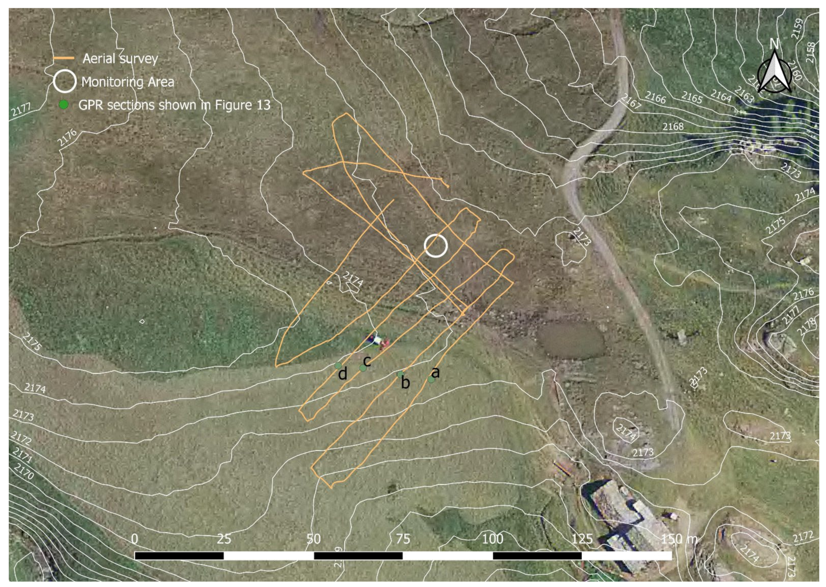
3.1. Cheneil Test Site

Cheneil is a little remote village in Valle d’Aosta, Italy, not reachable by car. The relatively large valley floor makes the site suitable for snow-cover mapping tests.
The survey was performed on 11 February 2021, on a hectare-wide gentle slope, as shown in Figure 2.
The map in Figure 3 shows the GPS-referenced locations of the aerial survey, ground-coupled surveys, and manual measurements. While the area of investigation is about 1 hectare, the total length of the aerial survey is above 2 km, allowing us to investigate the site with a relatively dense grid. The grid is not equally spaced, because the flight trajectory was manually controlled. The implementation of automatic flight mode, which improves the reliability and efficiency of the survey, has been upgraded after the tests.
In the same area, we carried out two ground-based GPR survey lines, and we manually measured the snow depth at some stations along the profile, for calibration and comparison purposes.

3.2. Gressoney Test Site

Gressoney test site, Aosta Valley, Italy, is in a ski-resort area; the test site was selected because logistically convenient (ski lifts).Snow density and depth measurements had been performed during the test in a specific fenced area, as shown in Figure 4. The snow thickness was measured to be about 1 m, and the density ranged from 150 to 220 kg/m3.
The drone surveyed an area of about 0.4 hectares, flying inside and outside the monitored area, as in Figure 5. The pilot manually controlled the flight, maintaining the vehicle at about 3 m of height.

4. Results

4.1. Cheneil Test Site: Calibration

A first ground-based GPR acquisition and manual measurements of snow depth were performed to retrieve an estimate of snow velocity, and to have a solid reference to compare with GPR data acquired from the drone.
The main bang of the GPR signal is observed at the travel times of 2 ns, while the reflection event due to the snow–terrain interface is well depicted in the travel times range between 6 and 9 ns. The overall quality of the sections is rather good, allowing accurate picking of the main bang and the reflection of the terrain.
The ground-based survey along the two selected sections was calibrated by manual and punctual measurements of the snow depth by using a graduated rod. This calibration allowed us to estimate the average wave velocity by comparing the travel times of the GPR signals and the punctual snow depth measurements. The best-fitting between the two data sets is obtained for a wave velocity of about 0.26 +/− 0.005 m/ns, as reported in Figure 6.

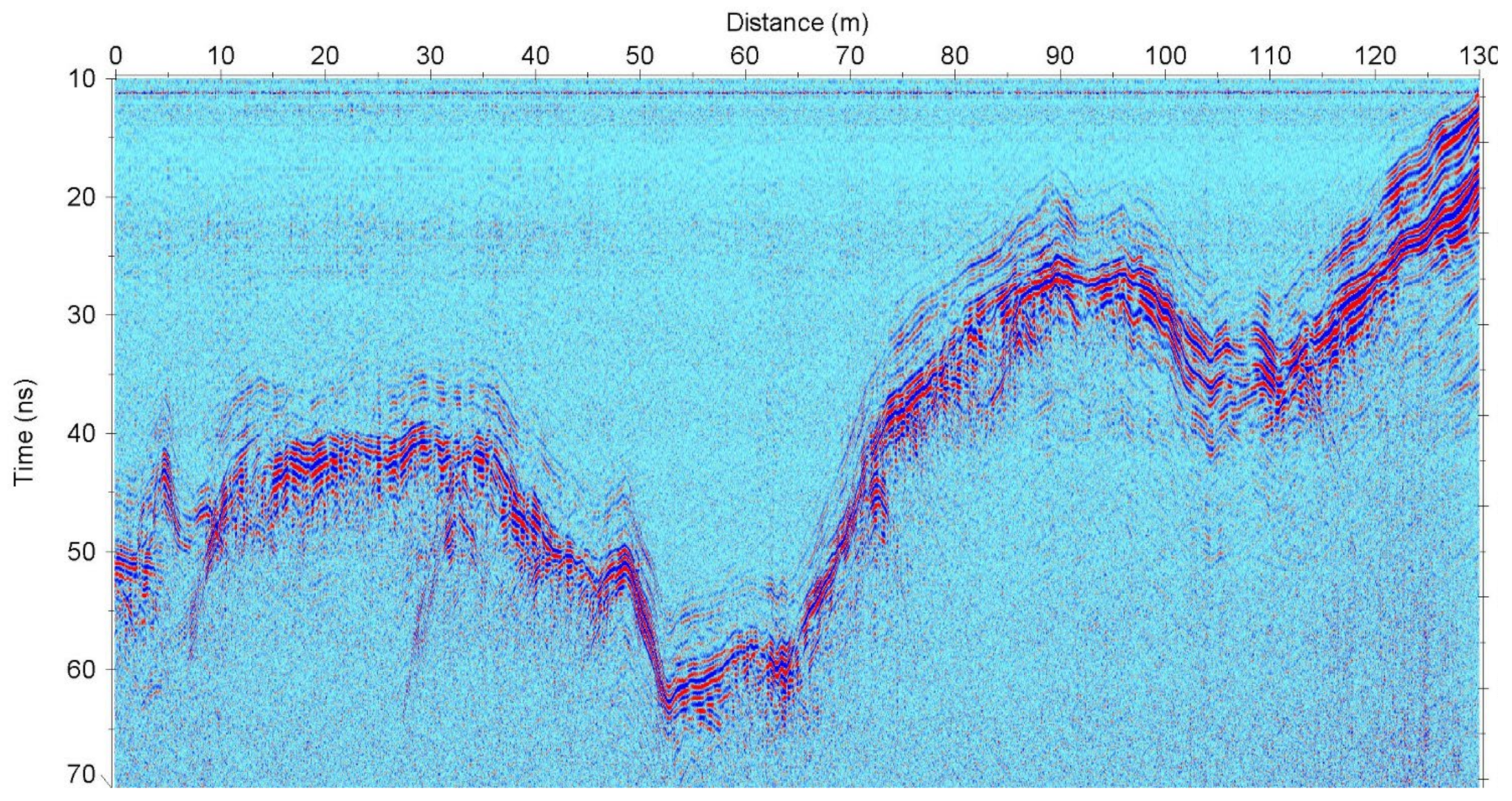
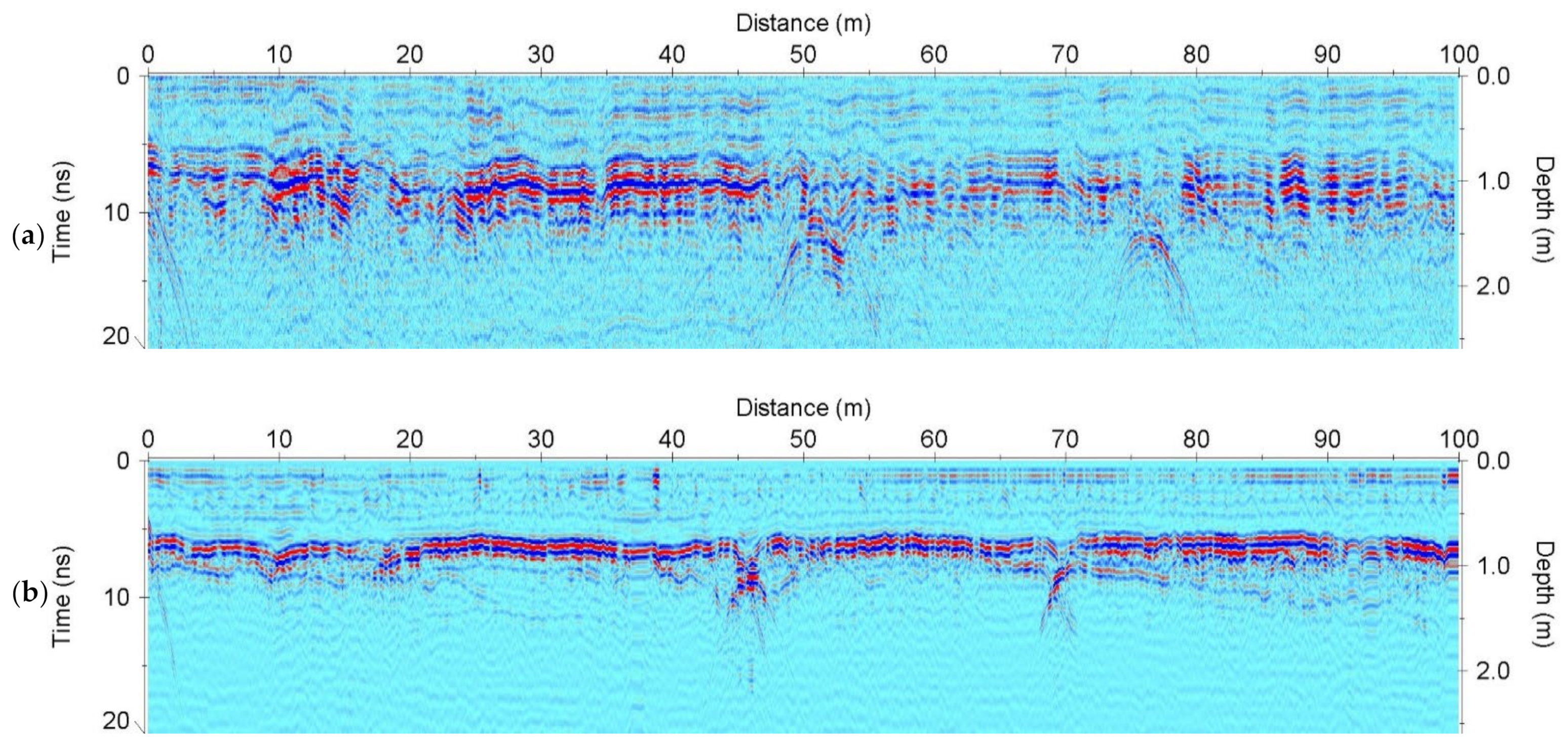
4.2. Cheneil Test Site: Sections from Drone

Some selected sections are given as examples in this paragraph. Two sections (line 3 and line 4 of the dataset) are clearest and are depicted in Figure 7 and Figure 8; the other sections are qualitatively similar.
The section of Figure 8 shows the reflection event of the snow–air interface, at travel times around 26–28 ns in the first part of the transect. An abrupt change of the flight altitude, caused by a sudden variation on the slope of the terrain at the relative coordinate of 120 m of the section, is also well depicted.
The section of Figure 7 shows the effect on the GPR data by changing again the altitude of the flight; the acquisition during the landing is also shown at the end of the section itself. The overall quality of the data acquisition appears satisfactory also for high flight altitudes, as pointed out in the center of the section. At coordinates between 50 and 60 m, the snow–air interface is picked up at the travel times of about 50–55 ns, corresponding to a flight elevation of about 7.5–8.0 m.
To highlight the reflection event caused by the interfaces between the air and the snow, and between the snow and the ground, we have included in the data processing flow-chart the radargram-staking to enhance the signal-to-noise ratio. We stacked about 9–11 radargrams for each transect. This leads to an average distance between two adjacent radar radargrams along each transect of about 20–25 cm.
The depicted sections demonstrate the capability of the prototype to image the snow thickness, even if the flight altitude is over 5 m. However, the system is not able to perfectly detect the air–snow interface, and one may misplace the interface position by a few tens of centimeters in some areas when performing the manual picking. For example, see Figure 7 at the relative coordinate of 4–6 m of the section.
The last processing step of the GPR sections acquired from the drone is to subtract the flight altitude, retrieved from the manual picking of the air–snow interface. In this way, the resulting sections become very similar to those acquired during a ground-based GPR survey. A comparison between the ground-based and drone-based GPR sections is shown in Figure 9.
The mismatch in the position of the hyperbolas in Figure 9a,b is similar, mainly due to the curvilinear path followed by the drone, as shown in the map in Figure 3. This issue does not affect the snow thickness 2D mapping, since every radargram is geolocalized. We can also point out that the drone-based section suffers from a loss of resolution compared to the ground-based one. We explain this difference because of optimum coupling between the antenna with snow for the snow-based survey, which cannot obviously be replicated in the drone base survey.

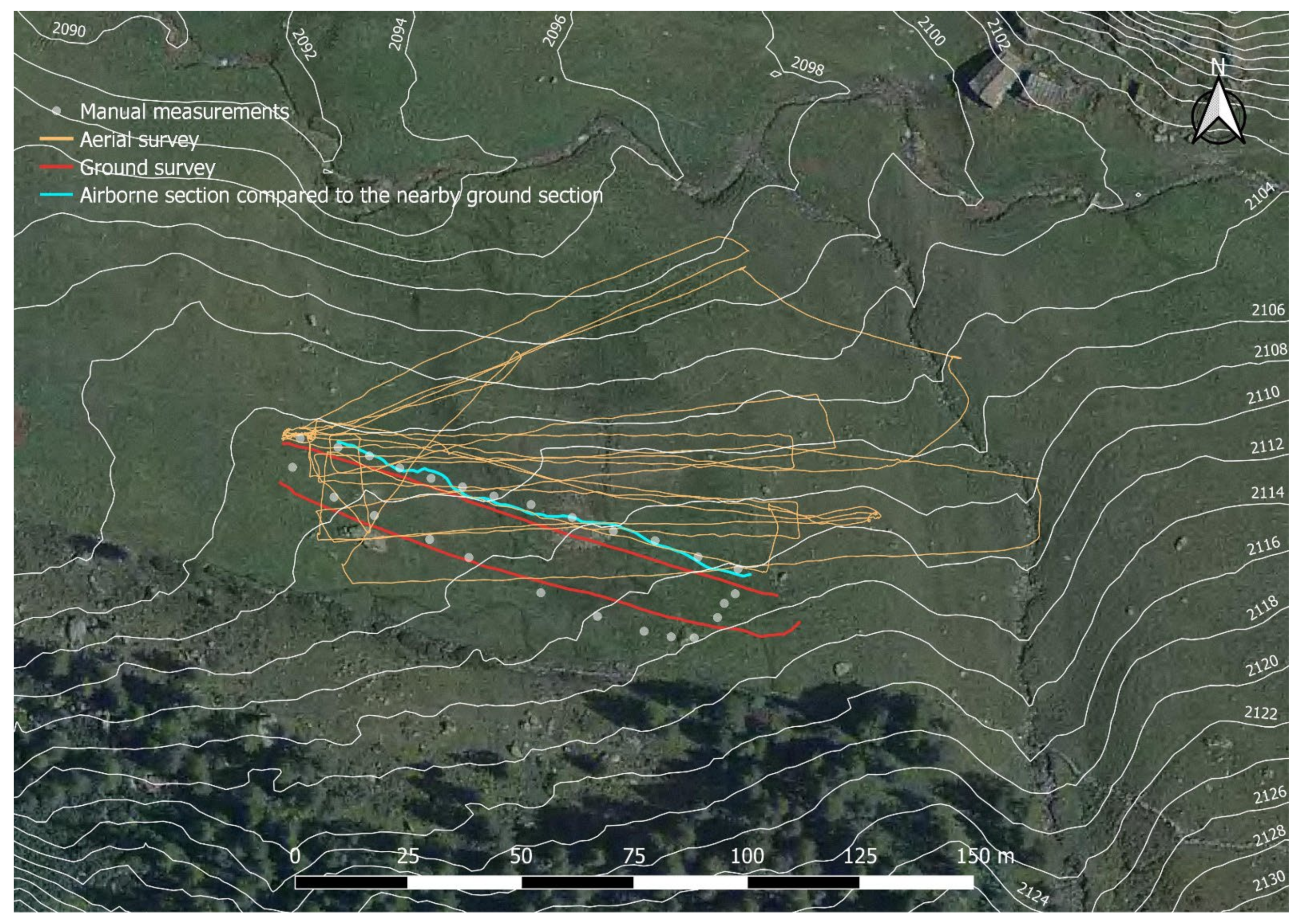
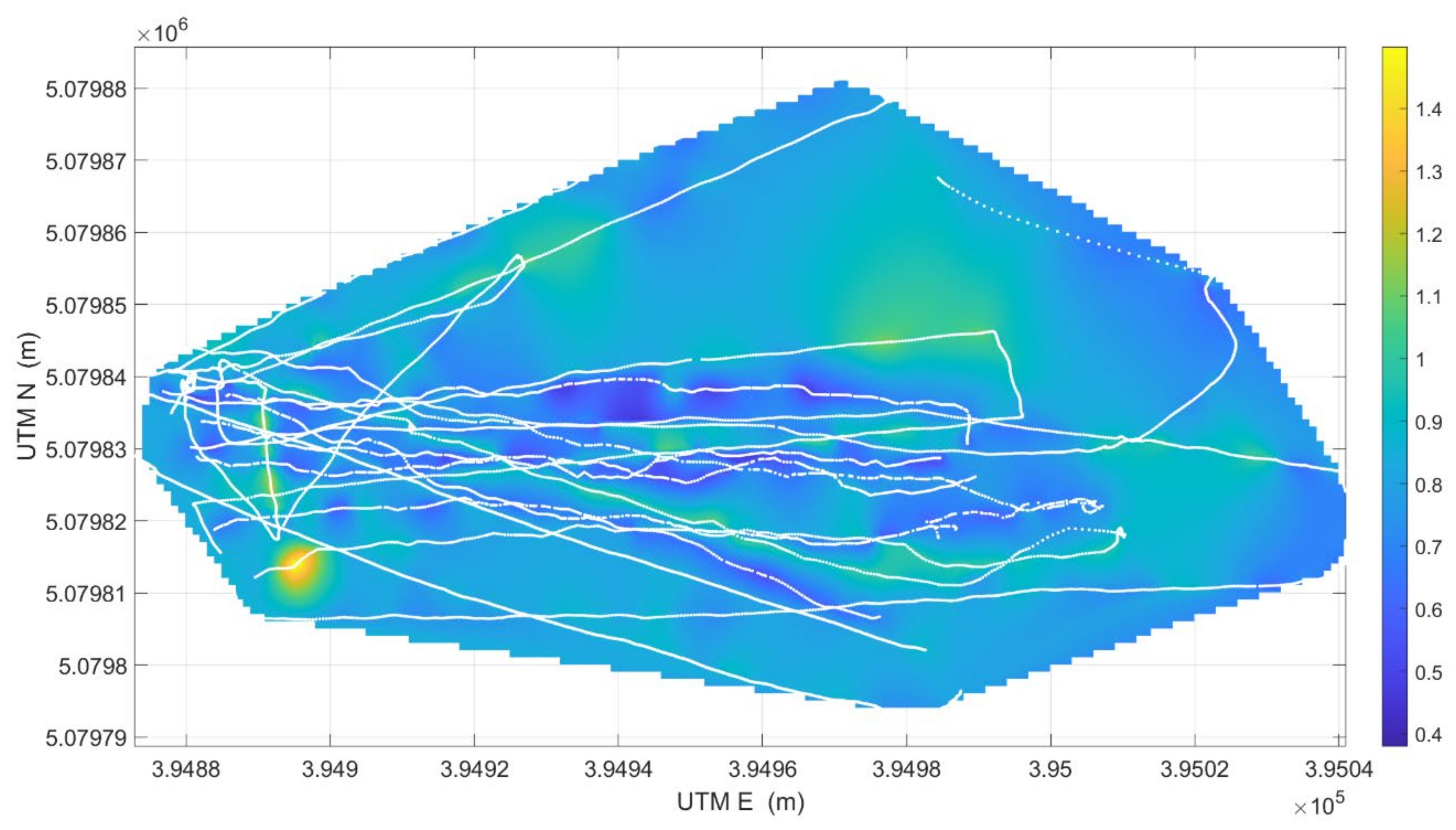
4.3. Cheneil Test Site: Mapping

The mapping of the snow depth has been performed after picking the differences in travel times between the air–snow interface reflection and the snow–ground reflection. The travel times have been converted to snow depth according to the velocity value estimated during the calibration step (0.26 m/ns).
We interpolated on a regular grid the snow depth the scattered GPR data. The grid nodes are represented by pixels of 0.5 m × 0.5 m. The maps of the distribution of the snow dept are reported in Figure 10.

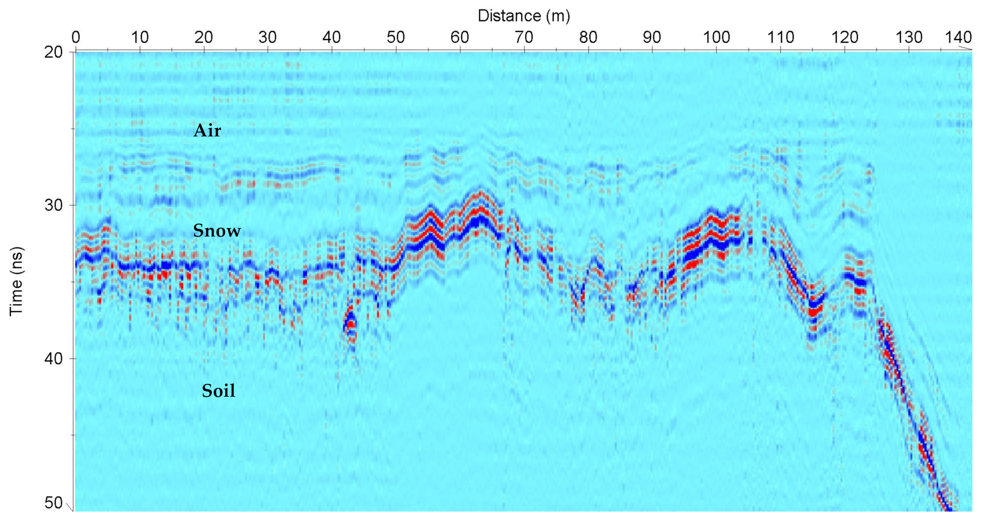
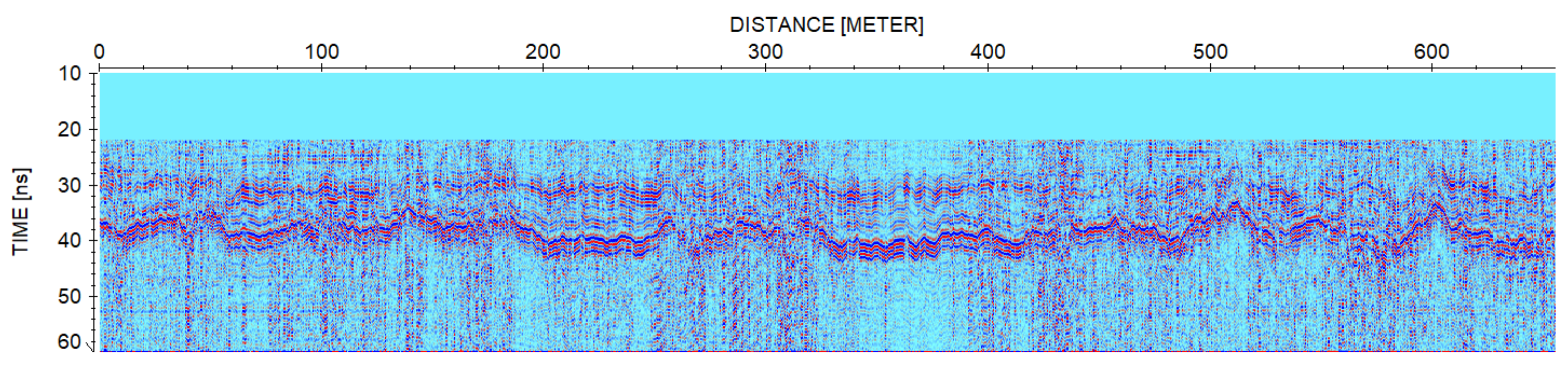
4.4. Gressoney Test Site

In the Gressoney test site, the section pictures were of poorer quality compared to the Cheneil test, in particular regarding the air–snow interface. We speculate that the density of the snow, quite low in both sites, causes a low reflection of the signal at the interface (dielectric permittivity of Gressoney snow ε = 1.3 and air ε = 1). Therefore, we checked the accuracy of the manual picking of the air–snow interface, comparing the results with rangefinder data acquired simultaneously by the drone telemetry system. Indeed, we selected the best section available, to compare rangefinder and GPR and evaluate the accuracy of the latter. It was acquired over the area in Figure 5, and it is shown in Figure 11. In some parts, the air–snow interface is difficult to see even after post-processing.

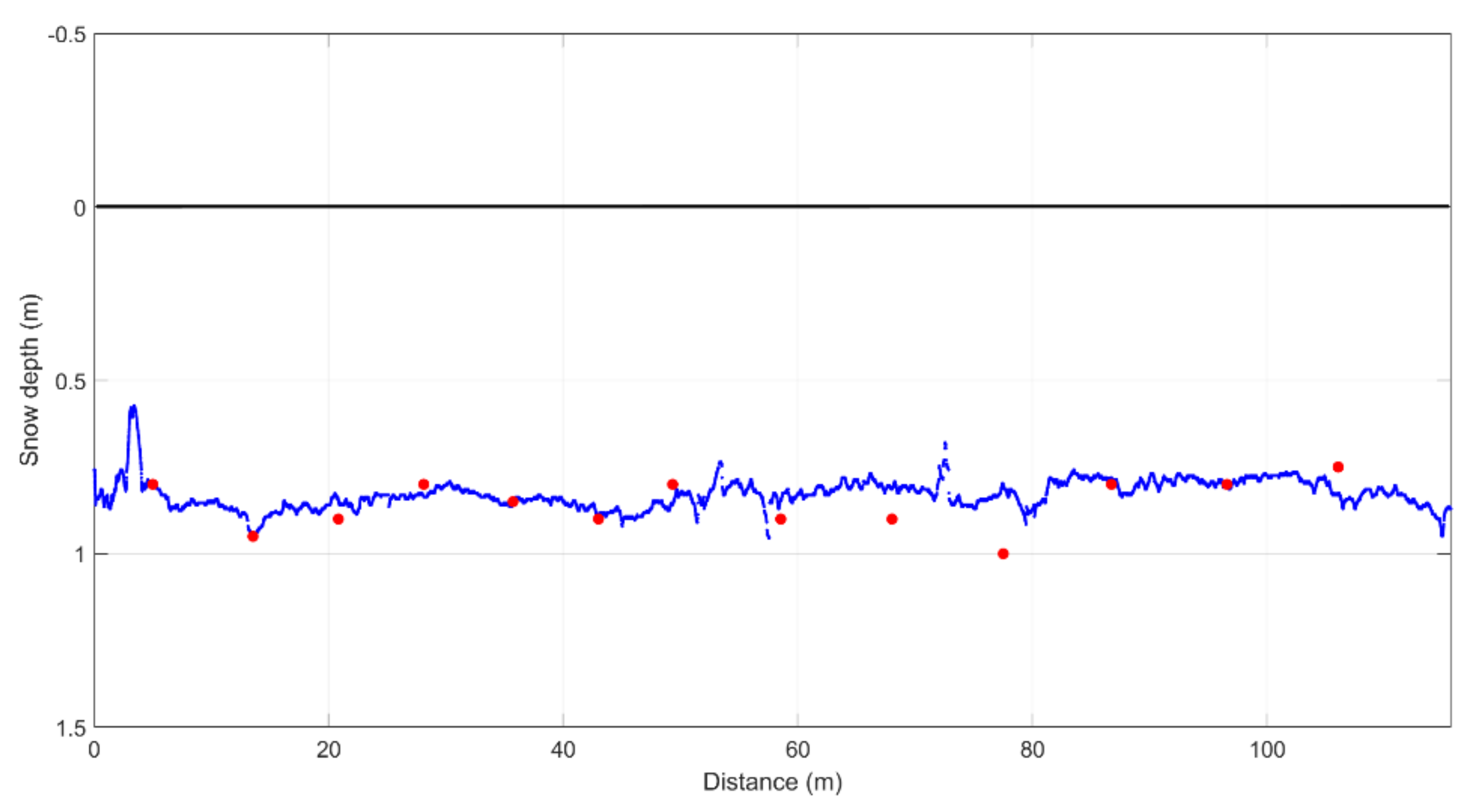
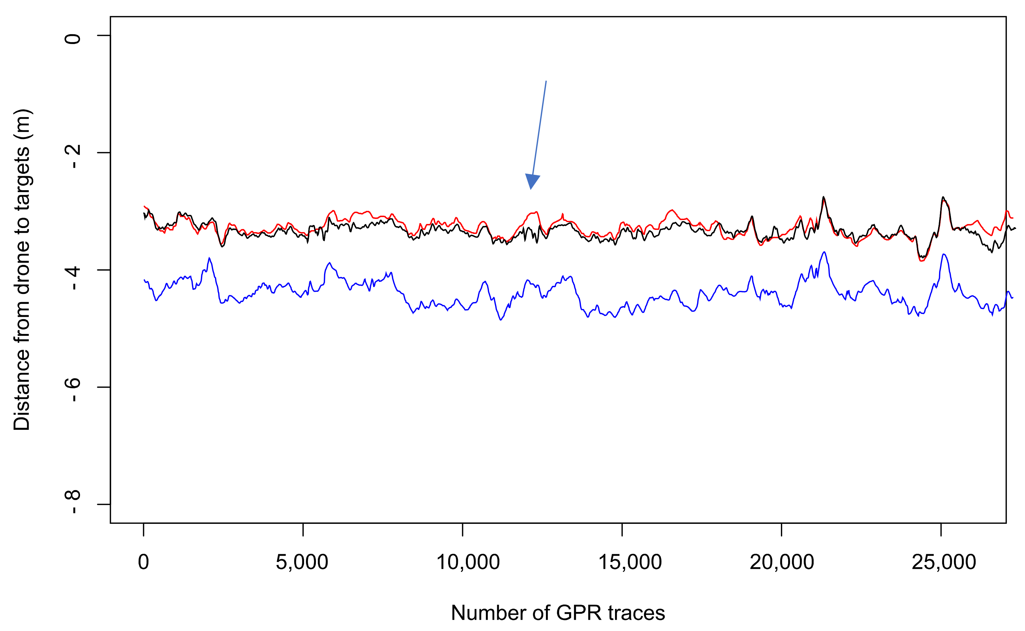
4.5. Gressoney Test Site: Calibration GPR-Rangefinder

The graph in Figure 12 shows the pickings of the two reflection events: in red, the air–snow interface by GPR; in blue, the snow–ground interface by GPR; in black, the air–snow interface by rangefinder. An accurate evaluation of the synchronism of the two different instruments was needed. Besides, it was important to accurately estimate the main bang time (7.75 ns +/− 0.025 ns) and to measure the relative position of the GPR antenna and the rangefinder (the latter is 7 cm above the base of the antenna, in this prototype configuration).
After subtracting the flight altitude from the radargrams, the GPR sections become more familiar, similar to the ground-based ones. Four parallel sections are shown in Figure 13, and their position is highlighted in Figure 5. The electromagnetic wave velocity was estimated with Looyenga’s equation [27,28,29] to be about 0.26 m/ns, considering an average snow density of 180 kg/m3, since manual measurements reported values from 150 to 210 kg/m3.

4.6. Gressoney Test Site: Mapping

A georeferenced map of the area was drawn in Figure 14, with similar interpolation processing to Figure 10. The snow depth was calculated using the GPR pickings for the snow–ground interface and the rangefinder data for the air–snow interface, estimated to be more precise than the manual GPR pickings. The time-depth conversion, with the velocity estimated with Looyenga’s equation, was successfully verified: in the monitored fenced area, highlighted in Figure 14 with a white circle, the GPR depth and the manually measured depth (about 1 m) were coincident.

5. Discussion

The two surveys, performed with a drone-borne GPR setup, allowed to map the snow-cover thickness of the surveyed area. The snow depth is usually estimated using a ground-based GPR survey or manual measurements by using a graduate stick. The main advantage, compared to the standard investigation, is the speed of the data acquisition: the Gressoney acquisition lasted less than 10 min, whereas carrying a GPR over the same path using ground-based radar, on the soft snow, would require more time and effort for the operators.
The test sites were both safe conditions for a ground-based GPR survey. However, it was evident how the drone could rapidly acquire data on nearby slopes, rocks, or other unstable features, where the human intervention could pose the operator at risk. This solution can therefore open new possibilities to map the SWE in poorly accessible basins.

5.1. Resolution

One limitation of the setup was the inability to display the inner features of the snow stratigraphy. A better vertical resolving power could be achieved by adopting higher frequency antennas: a customized release of the commercial antennas up to 2 GHz could be easily implemented in our system, allowing us to double the vertical resolution. Recent research tested a specifically built antenna for airborne GPR surveys, designing a specific unambiguous range, range resolution, and frequency bandwidth [20]. Their results on the snow cover test point out that airborne surveys can reach good accuracy and resolution with an adequate design. However, such detailed resolution is not always required. For these cases, our work demonstrated that also standard commercial systems such as 2-channel GPR devices and 900 MHz antennae can provide adequate output.
As far as the horizontal resolution is concerned, we distinguish between the resolution in-line (along the transect) and off-line. The latter is a matter of the coverage density; this can be planned by designing an automatic-flight grid survey. In this case, the line spacing can vary from 1 m, or even below, to tens of meters, according to the resolution required and the time available. The in-line resolution is instead related to the performance of the radar system (repetition rate of the pulse and stacking option) and the flight velocity. The installed GPR was able to collect about 50 radargrams per second, which means an average distance between radargrams of 2 cm, at a flight speed of 1 m/s. The need to perform the horizontal averaging of the radargrams (stacking) to provide a readable final section reduces the theoretical lateral resolution to some decimeters. In case of need for more resolution, the simplest solution is to reduce the flight speed.

5.2. Accuracy

Accuracy in the snow depth estimate depends on the reliability in picking the travel times of the two events: the reflection at the snow–air interface and the reflection at the snow–terrain interface. The first event is not always well depicted in the GPR sections; this is due to the low reflection coefficient between the soft snow and the air. The reflected signal from the second interface (snow–ground) is usually of sufficient amplitude to make it possible for an accurate picking. The accuracy in picking the true snow–ground interface is also affected by the presence of a thin and sometimes iced layer covering the ground, because of frozen and melting cycles that typically occur at the snow–ground interface, particularly at the beginning of the winter season. This effect could determine the underestimation of the travel times making the interpretation of the snow cover less accurate, even if this issue is not strictly related to the use of the drone. According to our previous experiences in similar frames, this effect can introduce errors up to 10%.
A possible solution for detecting more accurately the air–snow interface was developed in the data post-processing and can be considered for future drone-based GPR setups. Since all drones are equipped with a rangefinder to detect the flight altitude, it is possible to use rangefinder data instead of GPR pickings of the air–snow interface, as in the graph in Figure 12. If properly automated, the joint processing of the GPR and the rangefinder data can be a useful tool to lower the subjectivity of the section interpretation. This task demonstrated that, since the drone is equipped with sensors for flight control, their data log can enhance GPR interpretation reliability. An excellent example found in literature is the use of pitch, roll, and yaw measurements on a helicopter-based GPR system, to deal with the uncertainties related to the flight oscillations [16].

5.3. Flight Altitude

In our tests, the flight altitude did not greatly affect the data quality, as instead reported by other authors (e.g., [18]). This is well depicted in Figure 7, where a maximum flight altitude of about 7.5 m was reached; the two reflection events, the snow–air interface and the snow–terrain interface can be properly depicted and picked up. However, even if the effect of the flight altitude does not apparently affect the quality of the radar section, the impact on the resolution could be relevant as the radiation footprint of the antenna (related to the Fresnel zone) is strictly related to the source-to-target distance. By increasing the distance, the geometrical spreading increase, and the footprint of the radiated energy on the snow increases as well, with an overall reduction in the transmitted energy into the snow. This effect could be greater at greater snow depths. When planning automatic-flight surveys; therefore, it is advisable to control the flight altitude in the range between 1–2 m from the snow surface. Our prototype was not already tuned to perform an automatic flight survey, but adding this option is quite straightforward with the current drone technology, and tests at low altitudes have already been performed after the surveys presented in this paper.

5.4. System Setup

The choice of the GPR antenna can also affect the readability of the sections. For ground-based surveys, the antenna choice is often based on frequency, which drives a compromise between penetration depth and resolution. For drone-based surveys, other aspects must be taken into account. One is the shielding of the antenna, which for commercial GPRs is not so easy to quantify without tests. For example, we found by preliminary tests that a 400 MHz antenna shows a much better signal-to-noise ratio, so it could be preferred to the 900 MHz antenna for some snow-mapping applications, even if the resolution is certainly worse. Besides, not all antennas can be mounted on a drone, due to payload limitations. According to our experience, long-shaped antennae such as the Subecho 70 MHz can be mounted on such drones, and their weight distribution is not an obstacle to a smooth flight, provided that flight parameters on the autopilot are properly tuned.

5.5. Logistical Issues

If one would like to estimate the reliability of upscaling of the method at the scale of the basin, we analyze a possible application to a real case. Our tests, while useful to understand eventual criticalities in drone-borne GPR surveys, did not reproduce the real-case conditions in which such systems may shine. For example, in surveys of relatively large areas, the resolution is not crucial, as often are the real cases of SWE measurements. First, an automatic flight plan could be planned in advance, based on satellite images, and loaded on the drone autopilot.
Once on the site, the preliminary preparation of the survey (inspection of the area and check-up of the devices) could require no more than 30 min. The flight speed can be set up to 5 m/s (in our prototype), and it should be fine with the in-line resolution required. A boustrophedon path with 10 m spacing could be performed, with stops every 15 min for battery replacement (which takes no more than 5 min). At least 6 battery pit-stops are required in our fictional example. Bringing enough batteries and a portable power generator is suggested, such that batteries can be charged while the drone is flying. According to these assumptions, an area of 25 hectares could be covered in about 3 h.
One aspect not yet investigated in this research is the reliability of the system for acquiring accurate data on high-slope terrain. Our test sites did not exceed 20° of slope, and we found no critical issue in the acquisition. However, critical problems should be addressed when flying on much higher slopes. First, flight safety can be compromised. The current setup has only one sensor measuring the distance from the ground vertically; thus, horizontal sensors should be added to control and maintain a safe distance from the nearby rock walls or obstacles. Then, the GPR sections could become difficult to read, because the transmitted signal has a conical shape, and therefore does not interact optimally with the topography. A system that tilts the antenna according to the slope could address this issue, requiring prior knowledge about the topography (i.e., a Digital Elevation Model), but the design and implementation could be difficult and expensive.

6. Conclusions

Our research discussed the methodology of drone-borne GPR acquisition for snow cover mapping in alpine environments. In particular, we tested a commercial antenna (900 MHz) not specifically designed for air-coupled applications. The study was able to identify the air–snow interface and the snow–ground interface, although the air–snow interface was not always easy to distinguish, due to the slight impedance mismatch between air and soft snow. The results were compared to ground-coupled GPR sections, while manual measurements served as wave-speed calibration. Since the results did not deviate from real values over 10%, we found the technology to be reliable in this context. Additionally, as demonstrated in the Gressoney test, the rangefinder sensor can be used when the small reflections from the air–snow interface are difficult to display.
This research, even if it is just a preliminary test, extends the experience of the geophysical community in the use of drones for glaciological applications. Drone-borne GPR technology is found to have advantages compared to ground-based surveys, especially in terms of speed and operator safety. In terms of resolution, the obstacles can be reasonably handled in flat or gently sloped terrain, if accuracy and precision requirements are not critical.
One limitation was the poor vertical resolution, which prevented detailed information about snow stratigraphy from being detected. This was due to the choice of using a commercial radar antenna, which many geoscientists already use, and although previous research has improved resolution, it requires a specific antenna design, which is costly and difficult to obtain. Future work could improve clarity and reliability in data collection by the setup of an automatic flight mode, which can survey large areas at a fixed height over the ground surface, and with a regular grid. Moreover, survey capabilities can be extended further by using different GPR antennas or different sets of GPR antennas, carried by the drone. Our future research will involve the study of a lower-frequency antenna (400 MHz), which has been found to display clear sections in preliminary tests.
At this stage of the development of the prototype, the main critical issue, a limitation that could limit the diffusion of the technology, is the amount of initial effort to tune a production-ready system based on drone-borne GPR. Additionally, the operators, from the manufacturer to the pilot to the data analyst, have to acquire solid experience in handling the system, to constantly achieve satisfying results.

Supplementary Materials

The following supporting information can be downloaded at: https://www.mdpi.com/article/10.3390/rs14071763/s1, Dataset: Drone-borne GPR data for snow-thickness mapping, at Gressoney (Italy).

Author Contributions

Conceptualization, D.F.; methodology, D.F, A.V. and A.G.; software, A.V. and A.G.; validation, A.G. and A.V.; formal analysis, A.V. and A.G.; investigation, D.F. and A.V.; resources, A.G. and D.F.; data curation, A.V. and A.G.; writing—original draft preparation, A.G. and A.V.; writing—review and editing, A.V. and A.G.; visualization, A.V and A.G.; supervision, A.G.; project administration, A.G. and D.F.; funding acquisition, A.G. All authors have read and agreed to the published version of the manuscript.

Funding

This research was funded in the activities of the “CC-Glacier lab” laboratory of the Department of Excellence of the Politecnico di Torino—DIATI, funded by Italian Government—Ministry of Research with DM 262-11 May 2017 and Note of Funding of 10 January 2018.

Institutional Review Board Statement

Not applicable.

Informed Consent Statement

Not applicable.

Data Availability Statement

A dataset (GPR data) generated for this study is available as Supplementary Materials.

Acknowledgments

We acknowledge Alessandro Ainardi for piloting the drone and for helpful discussion about the aerodynamics and stability of the drone. We acknowledge the contribution of Francesca Pace for her kind support in drawing the state of the art of drone technology used for geophysical applications. A special thanks to Fabrizio Troilo (Fondazione Montagna Sicura), for his help during the acquisitions and the manual measurements of snow depth at the Cheneil test site. Thanks to Monterosa Ski S.p.a. for their logistical support in the Gressoney test site.

Conflicts of Interest

The authors declare no conflict of interest.

References

  1. Marshall, H.-P.; Schneebeli, M.; Koh, G. Snow Stratigraphy Measurements with High-Frequency FMCW Radar: Comparison with Snow Micro-Penetrometer. Cold Reg. Sci. Technol. 2007, 47, 108–117. [Google Scholar] [CrossRef]
  2. Rodriguez-Morales, F.; Byers, K.; Crowe, R.; Player, K.; Hale, R.D.; Arnold, E.J.; Smith, L.; Gifford, C.M.; Braaten, D.; Panton, C.; et al. Advanced Multifrequency Radar Instrumentation for Polar Research. IEEE Trans. Geosci. Remote Sens. 2014, 52, 2824–2842. [Google Scholar] [CrossRef]
  3. Kim, Y.; Reck, T.J.; Alonso-del Pino, M.; Painter, T.H.; Marshall, H.-P.; Bair, E.H.; Dozier, J.; Chattopadhyay, G.; Liou, K.-N.; Chang, M.-C.F.; et al. A Ku-Band CMOS FMCW Radar Transceiver for Snowpack Remote Sensing. IEEE Trans. Microw. Theory Tech. 2018, 66, 2480–2494. [Google Scholar] [CrossRef]
  4. Godio, A.; Rege, R.B. The Mechanical Properties of Snow and Ice of an Alpine Glacier Inferred by Integrating Seismic and GPR Methods. J. Appl. Geophys. 2015, 115, 92–99. [Google Scholar] [CrossRef]
  5. Godio, A.; Rege, R.B. Analysis of Georadar Data to Estimate the Snow Depth Distribution. J. Appl. Geophys. 2016, 129, 92–100. [Google Scholar] [CrossRef]
  6. Giordan, D.; Adams, M.S.; Aicardi, I.; Alicandro, M.; Allasia, P.; Baldo, M.; De Berardinis, P.; Dominici, D.; Godone, D.; Hobbs, P.; et al. The Use of Unmanned Aerial Vehicles (UAVs) for Engineering Geology Applications. Bull. Eng. Geol. Environ. 2020, 79, 3437–3481. [Google Scholar] [CrossRef] [Green Version]
  7. Yan, J.-B.; Gomez-Garcia Alvestegui, D.; McDaniel, J.W.; Li, Y.; Gogineni, S.; Rodriguez-Morales, F.; Brozena, J.; Leuschen, C.J. Ultrawideband FMCW Radar for Airborne Measurements of Snow Over Sea Ice and Land. IEEE Trans. Geosci. Remote Sens. 2017, 55, 834–843. [Google Scholar] [CrossRef]
  8. Yankielun, N.; Rosenthal, W.; Davis, R.E. Alpine Snow Depth Measurements from Aerial FMCW Radar. Cold Reg. Sci. Technol. 2004, 40, 123–134. [Google Scholar] [CrossRef]
  9. Tan, A.; Eccleston, K.; Platt, I.; Woodhead, I.; Rack, W.; McCulloch, J. The Design of a UAV Mounted Snow Depth Radar: Results of Measurements on Antarctic Sea Ice. In Proceedings of the 2017 IEEE Conference on Antenna Measurements & Applications (CAMA), Tsukuba, Japan, 4–6 December 2017; pp. 316–319. [Google Scholar]
  10. Tarchi, D.; Guglieri, G.; Vespe, M.; Gioia, C.; Sermi, F.; Kyovtorov, V. Mini-Radar System for Flying Platforms. In Proceedings of the 2017 IEEE International Workshop on Metrology for AeroSpace (MetroAeroSpace), Padua, Italy, 21–23 June 2017; pp. 40–44. [Google Scholar]
  11. Grab, M.; Bauder, A.; Ammann, F.; Langhammer, L.; Hellmann, S.; Church, G.J.; Schmid, L.; Rabenstein, L.; Maurer, H.R. Ice Volume Estimates of Swiss Glaciers Using Helicopter-Borne GPR—An Example from the Glacier de La Plaine Morte. In Proceedings of the 2018 17th International Conference on Ground Penetrating Radar (GPR), Rapperswil, Switzerland, 18–21 June 2018; pp. 1–4. [Google Scholar]
  12. Dematteis, N.; Troilo, F.; Grab, M.; Maurer, H.; Giordan, D. Identification of Bedrock Topography-Related Ice Fractures in the Planpincieux Glacier Using Helicopter-Borne GPR and DTM Analysis. In Proceedings of the 2021 IEEE International Geoscience and Remote Sensing Symposium IGARSS, Brussels, Belgium, 11–16 July 2021; pp. 1043–1046. [Google Scholar]
  13. Rutishauser, A.; Maurer, H.; Bauder, A. Helicopter-Borne Ground-Penetrating Radar Investigations on Temperate Alpine Glaciers: A Comparison of Different Systems and Their Abilities for Bedrock Mapping. Geophysics 2016, 81, WA119–WA129. [Google Scholar] [CrossRef]
  14. Merz, K.; Green, A.G.; Buchli, T.; Springman, S.M.; Maurer, H. A New 3-D Thin-skinned Rock Glacier Model Based on Helicopter GPR Results from the Swiss Alps. Geophys. Res. Lett. 2015, 42, 4464–4472. [Google Scholar] [CrossRef]
  15. Grab, M.; Mattea, E.; Bauder, A.; Huss, M.; Rabenstein, L.; Hodel, E.; Linsbauer, A.; Langhammer, L.; Schmid, L.; Church, G.; et al. Ice Thickness Distribution of All Swiss Glaciers Based on Extended Ground-Penetrating Radar Data and Glaciological Modeling. J. Glaciol. 2021, 67, 1074–1092. [Google Scholar] [CrossRef]
  16. Langhammer, L.; Rabenstein, L.; Schmid, L.; Bauder, A.; Grab, M.; Schaer, P.; Maurer, H. Glacier Bed Surveying with Helicopter-Borne Dual-Polarization Ground-Penetrating Radar. J. Glaciol. 2019, 65, 123–135. [Google Scholar] [CrossRef] [Green Version]
  17. Li, C.J.; Ling, H. High-Resolution, Downward-Looking Radar Imaging Using a Small Consumer Drone. In Proceedings of the 2016 IEEE International Symposium on Antennas and Propagation (APSURSI), Fajardo, PR, USA, 26 June–1 July 2016; pp. 2037–2038. [Google Scholar]
  18. Cabrera, R.A.; Bekic, G. Drone-Borne Ground-Penetrating Radar Suitability for Specific Surveys: A Comparative Study of Feature Sizes versus Antenna Frequency and Elevation over the Ground. First Break 2018, 36, 83–89. [Google Scholar] [CrossRef]
  19. Jenssen, R.O.R.; Eckerstorfer, M.; Jacobsen, S.; Storvold, R. Drone-Mounted UWB Radar System for Measuring Snowpack Properties: Technical Implementation, Specifications and Initial Results. In Proceedings of the International Snow Science Workshop, Innsbruck, Austria, 7–12 October 2018. [Google Scholar]
  20. Jenssen, R.O.R.; Eckerstorfer, M.; Jacobsen, S. Drone-Mounted Ultrawideband Radar for Retrieval of Snowpack Properties. IEEE Trans. Instrum. Meas. 2020, 69, 221–230. [Google Scholar] [CrossRef] [Green Version]
  21. Oborne, M. Mission Planner; ArduPilot Dev Team: Canberra, ACT, Australia, 2021. [Google Scholar]
  22. TeamViewer; TeamViewer: Göppingen, Germany, 2021.
  23. Riley, E.J.; Lenzing, E.H.; Narayanan, R.M. Characterization of Radar Cross Section of Carbon Fiber Composite Materials. In Radar Sensor Technology XIX; and Active and Passive Signatures, VI; Ranney, K.I., Doerry, A., Gilbreath, G.C., Hawley, C.T., Eds.; International Society for Optics and Photonics: Baltimore, MD, USA, 21 May 2015; p. 946103. [Google Scholar]
  24. Sandmeier, K.-J. Reflexw; Sandmeyer Geophysical Research: Karlsruhe, Germany, 2021. [Google Scholar]
  25. Forte, E.; Dossi, M.; Colucci, R.R.; Pipan, M. A New Fast Methodology to Estimate the Density of Frozen Materials by Means of Common Offset GPR Data. J. Appl. Geophys. 2013, 99, 135–145. [Google Scholar] [CrossRef]
  26. Previati, M.; Godio, A.; Ferraris, S. Validation of Spatial Variability of Snowpack Thickness and Density Obtained with GPR and TDR Methods. J. Appl. Geophys. 2011, 75, 284–293. [Google Scholar] [CrossRef]
  27. Looyenga, H. Dielectric Constants of Heterogeneous Mixtures. Physica 1965, 31, 401–406. [Google Scholar] [CrossRef]
  28. Glen, J.W.; Paren, J.G. The Electrical Properties of Snow and Ice. J. Glaciol. 1975, 15, 15–38. [Google Scholar] [CrossRef] [Green Version]
  29. Godio, A. Georadar Measurements for the Snow Cover Density. Am. J. Appl. Sci. 2009, 6, 414–423. [Google Scholar] [CrossRef] [Green Version]
  30. R Core Team. R: A Language and Environment for Statistical Computing; R Foundation for Statistical Computing: Vienna, Austria, 2021. [Google Scholar]
  31. The MathWorks Inc. MATLAB; The MathWorks Inc.: Natick, MA, USA, 2021. [Google Scholar]
  32. QGIS Development Team. QGIS Geographic Information System; Open Source Geospatial Foundation: Chicago, IL, USA, 2021. [Google Scholar]
Figure 1. Scheme of the drone coupled with a 900 MHz antenna.
Remotesensing 14 01763 g001
Figure 2. The drone deployed in the Cheneil survey area.
Remotesensing 14 01763 g002
Figure 3. Cheneil survey map: aerial survey, ground survey, manual measurements. The blue line refers to the aerial section compared, in the results section, to the nearby ground-based section. Contour lines every 2 m. Map rendering with QGIS [32]. Base map: 2012 Ortophoto by Aosta Valley regional service geoCartoSCT.
Remotesensing 14 01763 g003
Figure 4. Gressoney test site. The monitored area with snow thickness and density measurements is delimited by rods and ropes.
Remotesensing 14 01763 g004
Figure 5. Gressoney survey map: the path of the aerial survey is painted in white. The white circle represents the small monitoring area where density and snow depth measurements are available. Contour lines every 1 m. Letters from a to d indicate GPR sections shown in the results section. Map rendering with QGIS [32]. Base map: 2012 Ortophoto by Aosta Valley regional service geoCartoSCT.
Remotesensing 14 01763 g005
Figure 6. Calibration of the snow velocity from pickings of ground-based GPR survey (blue line) and manually measured points (in red) along the transect #1. The best-fitting is obtained for velocity = 0.26 m/ns.
Remotesensing 14 01763 g006
Figure 7. Example of GPR section acquired from the drone (line #4).
Remotesensing 14 01763 g007
Figure 8. Zoom on the interfaces depicted by a drone GPR section (line #3).
Remotesensing 14 01763 g008
Figure 9. Comparison between drone-based (a) and ground-based (b) GPR sections over the same path. Paths are shown in Figure 3, and the ground-based profile was cut to match the beginning of the drone-based one. Three hyperbolas show the same (unidentified) targets under the snow. Comparing the hyperbolas positions, the match is good but suffers from the drone’s curvilinear path.
Remotesensing 14 01763 g009
Figure 10. Snow depth distribution calculated from aerial survey data and ground-coupled survey data. Values in the colour scale are expressed in meters. Data are slightly smoothed for better visualization.
Remotesensing 14 01763 g010
Figure 11. Section of the entire Gressoney survey (after the post-processing described in the Methods section, not corrected for the flight altitude). The accuracy in the detection of the air–snow interface is very poor in some parts, e.g., at 250–300 m of relative coordinates, and at 420–480 m.
Remotesensing 14 01763 g011
Figure 12. Data was extracted from Figure 11 by manually picking the air–snow interface (in red) and the snow–ground interface (in blue). The black line was retrieved by the rangefinder sensor log, appropriately synchronized with the GPR data. In some zones, the unclear reflection made the picking underestimate the flight altitude by 10–20 cm, up to 50 cm at a point indicated by an arrow.
Remotesensing 14 01763 g012
Figure 13. Four parallel sections of the Gressoney test sites after subtracting the flight altitude (letters (ad) correspond to the 4 GPR sections indicated in the bottom left of Figure 5).
Remotesensing 14 01763 g013
Figure 14. Snow depth distribution of Gressoney test site calculated from GPR pickings of snow–ground interface and data from rangefinder for the air–snow interface. Values in the colour scale are expressed in meters. The circle in the map highlights the monitoring area, where a manual measurement recorded 1 m depth (consistently with the mapped values). Data are slightly smoothed for better visualization.
Remotesensing 14 01763 g014
Table 1. Main features of the drone Venture VFF_H01 prototype.
Weight and Dimensions
Max take-off weight12 kg (estimated)
Max payload (including batteries)7 kg
Min container size500 × 500 × 500 mm (to be adapted to the size of the GPR antenna)
Height80 cm
Max width2 m
Flight equipment
Central bodyCarbon/ CNC machined light-alloy
Propellers (4×)28″ (diameter) × 9.2″ (pitch), foldable
Engines (4×)Brushless, Heavy-duty IP35
Batteries (2×)Li-Po Very high energy density, 6s 5p 2 × 9000 mAh (safe use: 7000 mAh)
AutopilotPixhawk2 with triple redundancy IMU system + embedded Raspberry companion computer
Laser altimeterRange 100 m, resolution 1 cm
TelemetryMicrohard P2400, range 20 km, 1 W
Radio controlYeti DS24 Hall effect Joystick, configured on LAN
Protection for internal electronic componentsAgainst dust and water splashes
Flight performances
Flight duration without payload with two batteries (15% remaining charge, sea level, stationary flight without wind)50 min
Flight duration with 6000 g payload with two batteries (15% remaining charge, sea level, stationary flight without wind)15 min
Max cruise speed12 m/s
Max wind for safe conditions8 m/s
Flight modesAutomatic
GPS-related manual
Constant height (>1 m) laser-assisted
Acquisition devices
GPR acquisition unit + GPR antenna 900 MHzFrontal camera
Onboard mini PCGPS
Publisher’s Note: MDPI stays neutral with regard to jurisdictional claims in published maps and institutional affiliations.

