Article

Combinations of Feature Selection and Machine Learning Algorithms for Object-Oriented Betel Palms and Mango Plantations Classification Based on Gaofen-2 Imagery

1
Key Laboratory of Practical on Tropical Crops Information Technology in Hainan, Chinese Academy of Tropical Agricultural Sciences, Institute of Scientific and Technical Information, Haikou 571000, China
2
Key Laboratory of Agricultural Remote Sensing, Ministry of Agriculture and Rural Affairs, Beijing 100100, China
*
Author to whom correspondence should be addressed.
Remote Sens. 2022, 14(7), 1757; https://doi.org/10.3390/rs14071757
Submission received: 2 March 2022 / Revised: 1 April 2022 / Accepted: 4 April 2022 / Published: 6 April 2022

Abstract

:
Betel palms and mango plantations are two crucial commercial crops in tropical agricultural areas. Accurate spatial distributions of these two crops are essential in tropical agricultural regional planning and management. However, the characteristics of small patches, scattering, and perennation make it challenging to map betel palms and mango plantations in complex tropical agricultural regions. Furthermore, the excessive features of very-high-resolution (VHR) imaging might lead to a reduction in classification accuracy and an increase in computation times. To address these challenges, we selected five feature selection (FS) methods (random forest means a decrease in accuracy (RFMDA), ReliefF, random forest-recursive feature elimination (RFE), aggregated boosted tree (ABT), and logistic regression (LR)) and four machine learning algorithms (random forest (RF), support vector machine (SVM), classification and regression tree (CART), and adaptive boosting (AdaBoost)). Then, the optimal combinations of FS and machine learning algorithms suited for object-oriented classification of betel palms and mango plantations were explored using VHR Gaofen-2 imagery. In terms of overall accuracy, all optimal classification schemes exceeded 80%, and the classifiers using selected features increased the overall accuracy between 1% and 4% compared with classification without FS methods. Specifically, LR was appropriate to RF and SVM classifiers, which produced the highest classification accuracy (89.1% and 89.88% for RF and SVM, respectively). In contrast, ABT and ReliefF were found to be suitable FS methods for CART and AdaBoost classifiers, respectively. Overall, all four optimal combinations of FS methods and classifiers could precisely recognize mango plantations, whereas betel palms were best depicted by using the RF-LR method with 26 features. The results indicated that combination of feature selection and machine learning algorithms contributed to the object-oriented classification of complex tropical crops using Gaofen-2 imagery, which provide a useful methodological reference for precisely recognizing small tropical agricultural patterns.

1. Introduction

Information on cropland extent is fundamental for crop monitoring and management [1]. Remote sensing technology can supply effective and accurate information about agricultural activity because of its characteristic of repeatability, timeliness, and high coverage [2], making it a primary data source for agricultural crop recognition [3,4]. Existing middle- or coarse-resolution remote sensing data have the disadvantage that the limited spatial resolution is insufficient to precisely classify patches with small agricultural crop size distributions [5]. Very-high-resolution (VHR) images have detailed textural and spatial information, providing an improved opportunity for precise classification of small croplands [6]. The object-based classification considers both spectral and also morphological, contextual, and proximity features in VHR images; therefore, many previous studies have indicated that object-oriented image analysis approaches outperformed pixel-based classifications when comparing accuracy metrics [7,8]. Numerous studies have used various object-oriented supervised machine learning classifiers for crop identification based on VHR satellite datasets [9,10]. The common machine learning algorithms include random forest (RF) [7], support vector machine (SVM) [8], classification and regression tree (CART), K-nearest neighbors (KNN) [11], adaptive boosting (AdaBoost) [12], neural networks, etc.
Object-based classification can lead to better performance using a high number of features generated from spectral, spatial, and contextual properties in VHR images [13]. Alternatively, to further improve classification accuracy, increasing amounts of auxiliary features (e.g., geometry, texture, and vegetation index) is used to recognize land cover types [14]. However, not all features have a positive influence on land cover classification. Several studies have found that excessive input features may reduce the classification accuracy and increase the computation time [15,16]. The feature selection (FS) technique is very effective in reducing redundant information, which aims to find the optimal subset of features with minimal redundancy and maximal relevance to the objects. Several FS methods have been widely used in object-based classification. For example, Laliberte et al. [17] compared three FS methods for object-based vegetation classification, and pointed out that classification tree analysis was most suited for mapping arid rangelands with UltraCam-L imagery. Cánovas-García and Alonso-Sarría [18] indicated that the Gini index was the most appropriate FS method for identifying agricultural landscape by Z/I-imaging DMC imagery. Ma et al. [19] showed that support vector machine-recursive feature elimination (SVM-RFE) could provide more useful features to perform better classification accuracy for an agricultural area mapping using unmanned aerial vehicle imagery. Overall, there is no general FS method available to obtain optimal features for various machine learning classifiers, regions with different climatic conditions, and different types of remote sensing data. Therefore, further studies of the utility and efficiency of the FS methods need to be conducted according to different research purposes.
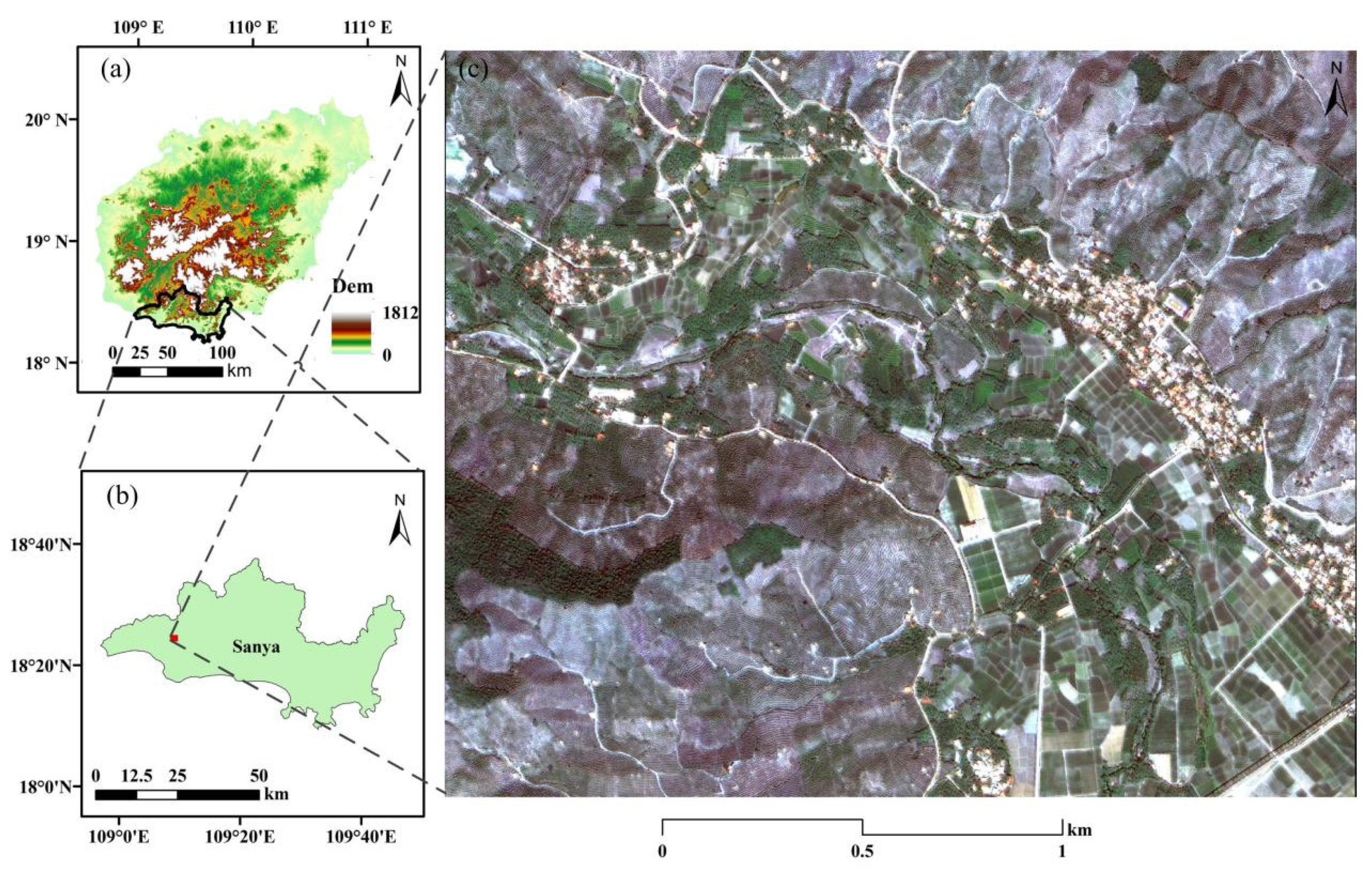
Betel palms and mango plantations are two important cultivated commercial crops in tropical and sub-tropical areas, such as Africa, China, India, Malaysia, and Thailand [20]. China is the world’s dominant producer of both betel nuts and mango, and the island of Hainan in southern China is the main production area of the two crops. The acreages of betel palms and mango plantations in Hainan grew from 26,944 and 36,076 ha, respectively, in 2000 to 115,171 and 56,934 ha, respectively, in 2019. Moreover, the total outputs of betel nuts and mango increased from 101,220 and 35,598 tons, respectively, in 2000 to 675,805 and 287,043 tons, respectively, in 2019 [21]. The industries of betel palms and mango plantations play a critical role in tropical rural economic development in Hainan due to their high profit margins and strong market demand [22]. To ensure a scientifically informed management policy relating to tropical crops, it is necessary to regularly monitor the accurate extents of betel palms and mango plantations. Compared with the temperate zone, the planting regions of tropical crops are relatively scattered and small, and more abundant crops present in a small area could reduce the spectral separability of different classes [23]. In addition, as two perennial evergreen trees, betel palms and mango plantations have no significant defoliation phase, unlike rubber plantations [24], which is another common tropical crop. Thus, it is a complex and challenging task to recognize betel palms and mango plantations in heterogeneous agricultural regions.
The Gaofen-2 satellite was launched from the Taiyuan Satellite Launch Centre on 19 August 2014, and is also the first civilian satellite with sub-meter spatial resolution and a 5-day repetition cycle in China [25]. The excellent spatial and temporal resolution of Gaofen-2 could provide more accurate spectral and textural information for detailed land cover mapping. In addition, compared with other foreign commercial satellites, Gaofen-2 data has the advantage of low cost, and some sectors (such as Chinese forestry, land, and resources) could obtain free satellite data [15]. Therefore, Gaofen-2 images have been widely used in agricultural monitoring [26,27]; however, these studies have mainly focused on a single crop type in temperate regions, such as wheat and maize. To the best of our knowledge, mapping tropical crops, especially for betel palms and mango plantations with Gaofen-2 imagery, has rarely been reported in previous literature. Whether Gaofen-2 data can accurately recognize tropical crops in complex heterogeneous agricultural regions is a topic which still needs in-depth research.
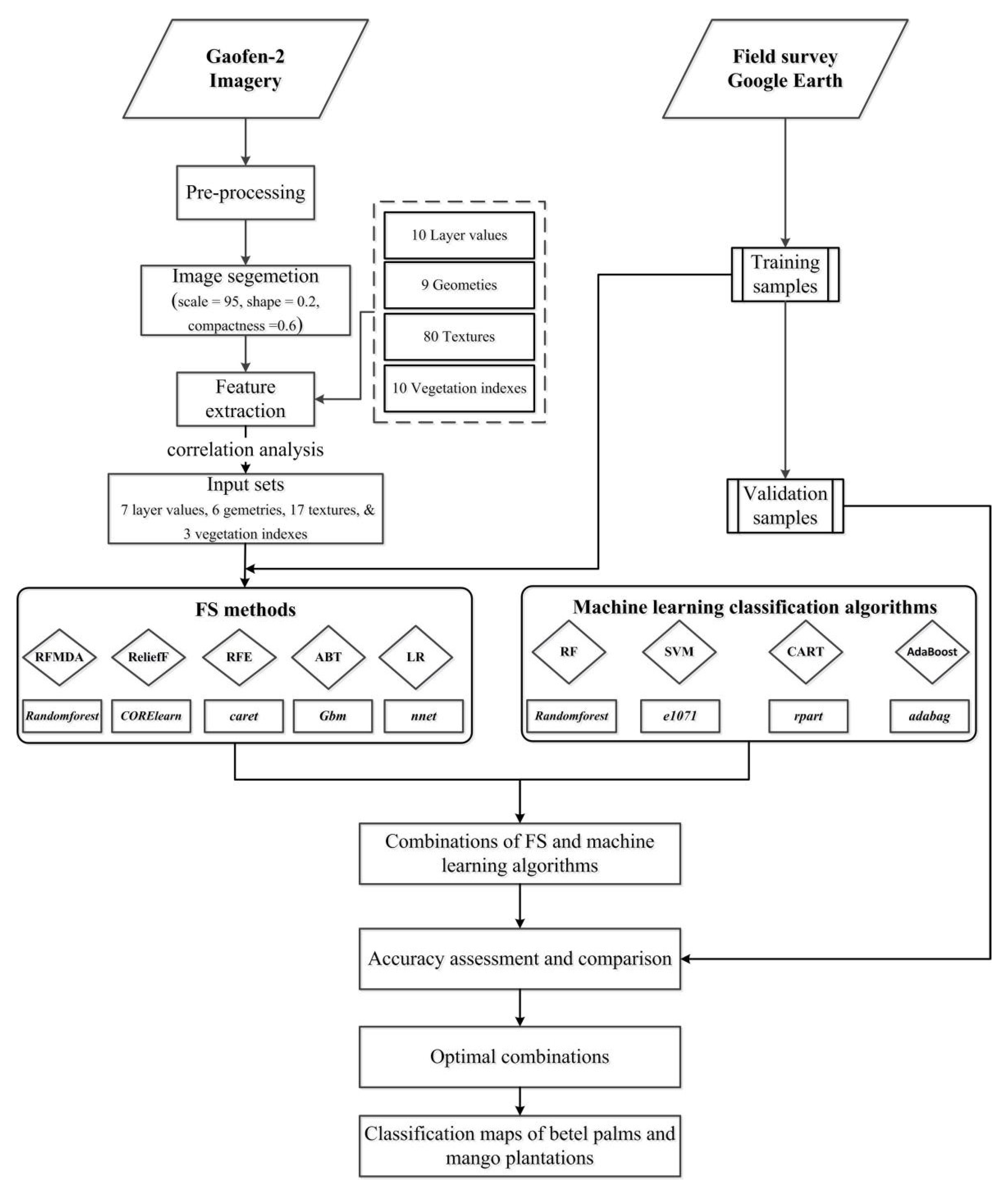
Our research aims to develop a framework for recognizing betel palms and mango plantations in complex tropical agricultural regions using Gaofen-2 imagery. The detailed objectives of this study are to: (1) evaluate the potential of GaoFen-2 imagery for mapping betel palms and mango plantations in complex tropical agricultural regions, (2) assess and compare the relative importance of different FS methods, and (3) explore the optimal combination of FS methods and machine learning classifiers for identifying betel palms and mango plantations.

2. Materials

2.1. Study Area

The study area is located southwest of the city of Sanya, Hainan Island, China (Figure 1a), which has a typical distribution of tropical agricultural plantations. The mean annual precipitation and mean annual temperature are 1347 mm and 25.7 °C, respectively, in the region, which belongs to the tropical monsoon climate. According to the 2020 Hainan Statistical Yearbook [21], the annual production of betel nuts in Sanya ranked fourth, while the annual mango production is more than 50% of the Hainan province’s mango yield. Although the experimental site only covers about 446 ha (Figure 1), it represents a typical characteristic of tropical agricultural region in southern Hainan Island. The main land cover types include mango plantations, betel palms, cultivated land (mainly vegetables), forest, built up (roads and residential buildings), and other land uses (e.g., water bodies and unutilized land).

2.2. Gaofen-2 Imagery

This study used a cloud-free Gaofen-2 image from 16 January 2020, with the Land Observation Satellite Data Service Platform of the China Center for Resource Satellite Data and Application (CASC, http://www.cresda.com/CN/ (accessed on 5 March 2020)). The resolutions of Gaofen-2 data are 1 m and 4 m in one panchromatic band and four multispectral bands, respectively. The detailed payload information about Gaofen-2 imagery is shown in Table 1 [26]. All imagery, including radiometric calibration, atmospheric correction, geometric rectification, and reprojection, was preprocessed in ENVI 5.3 software (Exelis Visual Information Solutions, USA). The fast line-of-sight atmospheric analysis of the spectral hypercubes (FLAASH) model was selected to perform the atmospheric correction [28]. The rational polynomial coefficients were used to execute geometric correction. The image was then georeferenced into UTM WGS84. In addition, a popular nearest neighbor diffusion (NNDiffuse) pan-sharpening method was used to generate multispectral imagery with a spatial resolution of 1 m. Then, the imagery was clipped to the study region for further analysis.

2.3. Samples

Ground reference samples included field surveys data using handheld global position system (GPS) receivers (Trimble Juno 3D) and visual interpretation data from Google Earth. In this study, we mainly evaluated the performance based on object-based classification. In order to avoid more than one class appearing in a single object, we selected the random samples according to ground reference data after the image was subjected to optimal segmentation (see Section 3.1). All samples selected for classification covered the entire study area to ensure unbiased estimation of all types in limited extent [29]. For detailed operation methods, please refer to our previous research [30]. The minimum number of samples was suggested to be 50 for each type when evaluating the classification accuracy [31]. Finally, a total of 3000 samples were supplied in the present study, ensuing approximately 500 sample points per class (six total classes). Then, the samples were randomly split into training and test samples at the ratio of 0.7:0.3. The training samples were used to construct the supervised classification models and adjust parameters of machine learning algorithms. Meanwhile, the test samples were applied in the accuracy assessment of mapping betel palms and mango plantations.

3. Methodology

The general workflow chart for mapping betel palms and mango plantations is summarized in Figure 2. First, the Gaofen-2 imagery was preprocessed in ENVI 5.3. The detailed interpretation of data preprocessing is shown in Section 2.2. Second, the image was segmented into objects using a multi-resolution segmentation algorithm in eCognition 9.0. Third, 109 initial features were chosen, including four types (layer values, geometry, texture, and vegetation index). Forth, five FS methods and four machine learning classification algorithms were applied in betel palms and mango plantations recognition using R software. Finally, the optimal combinations of FS and machine learning algorithms were evaluated to reduce the redundant features and obtain higher classification accuracy.

3.1. Image Segmentation and Features Extraction

In object-based classification, image segmentation mainly obtains the image objects by dividing them according to similar spatial and spectral characteristics, which effectively simulate the manual interpretation of imagery. For image segmentation, the most critical procedure is to select a suitable segmentation scale such that the object can clearly represent specific type of land use [32]. In the current study, we applied the estimation of scale parameter (ESP) tool to determine the optimal segmentation scales for delimiting the borders of different classes. The tool was provided by Dragut et al. [33] in order to maximize the heterogeneity of inter-segmentation and homogeneity of intra-segmentation. Finally, the optimum scale was set to 95 for tropical crop classification (Figure 3 and Figure 4). Then, a common multi-resolution segmentation algorithm in eCognition 9.0 was used to perform image segmentation, i.e., a bottom-up segmentation based on the fractal net evolution approach [34]. Besides the segmentation scale, two sets of key parameters needed to be determined: color/shape and compactness/smoothness. The color and shape mainly decide the spectral homogeneity of the object shape, where the sum of weight coefficient is equal to 1. While the compactness and smoothness control the compact edges and smooth boundaries [35], where the sum of weight coefficient is also equal to 1. In this paper, the parameters of color/shape and compactness/smoothness were set to 0.8/0.2 and 0.6/0.4, respectively.
To find suitable features for identifying betel palms and mango plantations, we selected 109 initial features based on the following four aspects: layer values, geometry, texture, and vegetation index. Detail features information is shown in Table 2. Gray-level co-occurrence matrix (GLCM) and gray-level difference vector (GLDV) are two very popular approaches for calculating textural features [36,37]. GLCM represents the frequency of various combinations of grey levels in an image object, and GLDV is the sum of GLCM within the image object on the diagonal [9]. The ten vegetation indexes have been commonly applied in agricultural researches, due to their potential to identify some crop field characteristic that may be vital to crop classification [38]. All features were calculated in eCognition 9.0. These features could provide abundant spectral, textural, and spatial features to determine optimal features for typical tropical vegetation classification. Previous studies have shown that the most important features were always highly correlated, which could lead to unstable classification results [39]. To reduce data redundancy of initial features, we calculated the correlations of all initial features using Spearman’s rank correlation coefficient, and those features for which the correlation coefficients were greater than 0.9 were eliminated, which has been commonly used in past studies on FS [17]. As a result, a total of 33 features remained in the present study (Table 3). All comparisons with FS methods and machine learning classifiers used the same features. Therefore, it is a reasonable assumption that the variations of classification accuracy were mainly caused by the different combinations of the FS method and machine learning algorithms.

3.2. FS Methods

Overall, there are three main categories of FS methods: filter, embedded technique, and wrapper [16]. Filter, as a simple and fast FS method, does not need any learning algorithm but rather selects optimal features on the basis of statistics. Wrapper mainly determines the most suitable features based on predictions by machine learning algorithms. The embedded method only requires one model to perform FS, achieving a computationally efficient approach compared with wrappers. In this study, we focused on assessing the following five FS methods, including three embedded methods (RFMDA, ABT, and LR) one filter (ReliefF), and one wrapper (RFE). We chose these five FS methods because they had been widely applied in feature optimization [16,19] due to their excellent performance. All FS methods were implemented in R software (version 4.0.2) through their respective packages (“randomforest”,“gbm”, “nnet”, “CORElearn”, and “caret” packages). Just as Li et al. [40] pointed out, it is usually safe practice to adopt the default parameters recommended by the software developers. Therefore, we also used the reference parameters in original sources of references when performing various FS methods.

3.2.1. Random Forest Mean Decrease in Accuracy (RFMDA)

The principle of random forest (RF) is establishing a set of decision trees by randomly selected features, where the single tree node may be called a forest [19,41]. RFMDA performs the feature quality assessment based on the difference among the original features and the modified features in which the approach randomly permutes values of observed data between examples using the mean decrease in accuracy. The above difference is then combined into an importance estimate for each tree in the forest, according to their influence on model accuracy [16]. The importance estimate for the feature is as follows:
I ( A j ) = d i n × ( S D d i / n )
where Aj represents the number of chosen feature, I(Aj) means the ultimate importance estimate result for feature Aj, i is the number of trees, di is the performance difference of the ith tree, n is the number of elements in the dataset, and SDdi means the standard deviation of di.

3.2.2. ReliefF

ReliefF is a common filter FS method that principally estimates the importance of features using a feature weight algorithm. Assuming that there is a total of m classes, class labels set can be considered as C = {C1, C2, …, Cm}. ReliefF mainly chooses a sample x from the training set D, and then finds the d-nearest samples from each class of x, forming the matrix M(c).
The specific formula of Relief-F is as follows [42]:
ω t = ω t x H d i f f ( t , S i , x ) r d + c c l a s s ( s i ) [ p ( c ) 1 p ( c l a s s ( S i ) ) x M ( c ) d i f f ( t , S i , x ) ] / ( r d )
where ω t means the weight of feature t, Si is the selected data sample S, x represents the data point belong to near hits or near misses, d represents the number of nearest samples, r is the number of iterations, p(c) means the frequency of occurrence of class C, and p(class(si)) shows the probability that sample Si appertains a class. diff(*) can be computed as follows [43]:
d i f f ( t , S i , S j ) = | S i t S j t max t min t | ,   if   the   features   are   continuous   values
d i f f ( t , S i , S j ) = 0 S i t = S j t 1 S i t S j t ,   if   the   features   are   discrete   values

3.2.3. Recursive Feature Elimination (RFE)

The RFE method is an iterative greedy method that performs the FS based on backward feature elimination [44]. Its main principle is selecting the optimal feature subset through repeatedly building a model. When the chosen variable with the smallest score is removed, the above process is continued until all features have been traversed. The RFE will then form a feature ranking that shows the importance of each input feature [45]. During the execution of RFE, a machine learning classifier is needed to assess the importance of predictors. Therefore, we applied the RF approach as the base classifier. It should be noted that the chosen variables may not be unique because of the split difference in resampling for the RFE method. RFE with k-fold cross-validation was then applied to solve the problem of split difference. In our study, k was set to 10, and the number of complete sets of folds was set to 200.

3.2.4. Aggregated Boosted Tree (ABT)

De’ath (2007) proposed the ABT method, an extension of the boosted tree method. The predictor error of ABT can be evaluated from the out-of-bag data (see [46]). However, it could obtain better prediction accuracy than boosted trees or bagged trees [47]. The ABT predictors are performed in the following steps: predicting the new data based on a collection of boosted trees and then aggregating the results of predictions. The detailed formula is as follows:
V V = f ( P C s ) = m f m ( P C s ) = m ϕ m b ( P C s ; δ m )
where PCs are the ordinary principal components, φ m is the weight assigned to each tree node in the collection of boosted trees and determines the combination form of predictions from independent trees, the function b ( P C s ; δ m ) is the independent trees, and δ m represents the split variables [48]. The loss function L(VV, f(PCs)) illustrates the difference between the response of ABT and the actual value, which is used to select the optimal features [49].

3.2.5. Logistic Regression (LR)

LR is a log-linear model that is suited for FS or classification [50]. LR mainly reveals the relations among dependent and explanatory variables on the basis of fitting a regression model. The LR formula can be expressed as follows [51]:
P ( y i = J ) = 1 1 exp ( β 0 i + β 1 i x 1 + β 2 i x 2 + + β n i x n )
where J represents the baseline class; P(yi = J) refers to the probability that the yi belongs to the class J; (x1, x2, …, xn) represents the input vector of the explanatory variable; β0i is a constant; and β1i, β2i, …, and βni represent the regression coefficients suited for corresponding explanatory variables.

3.3. Machine Learning Classification Algorithms

In this study, four common classification algorithms were applied for mapping typical tropical vegetation, including RF, support vector machines (SVM), classification and regression tree (CART), and AdaBoost. RF, SVM. and CART are progressively used in agricultural crop recognition and excessive reports can be found [9,10]. AdaBoost is an adaptive machine learning algorithm, and previous studies [12] demonstrated its advantages and capabilities in classifying crop structures. The optimal parameters of classifiers were identified using cross-validation, which are shown in Table 4.
RF includes a set of tree classifiers in which each classifier is obtained by a random vector sampling from the input vector and the input vector is classified based on the most popular voting class [52]. The approach is more effective and robust against noise compared with single bagging or boosting classifiers. To perform the RF classifier, two important parameters, including the number of trees in the forest (ntree) and the number of random subsets of input features at each split (mtry), should be established [53].
SVM is a nonparametric classifier based on statistical learning theory. The principle of SVM is to evaluate the best separation of classes using the position of decision boundaries [54]. SVM performs a soft classification, and the classifier can obtain a good classification result from complicated and noisy input. When dealing with samples with high dimensions, a positive kernel function should be selected to save computational time [55].
CART mainly constructs binary trees using the impurity level of given data, with only two classes for each internal node output [56]. One of the important capacities for CART is to generate regression trees, which are constructed by recursively selecting the attribute with the lowest Gini index [57]. At each internal node, the tree’s leaf nodes in corresponding division regions are decided by related splitting rules.
AdaBoost was proposed by Freund and Schapire [58] in 1996, which performs boosting in an iterative approach. The level of weight associated with classes is very important in iterative processing. First, given that all classes are the same weight, the weight of correctly classified classes is then declined, whereas that of misclassified classes is improved in each iteration. Each classified class has a corresponding weight that can be used to evaluate the classification accuracy. Finally, the classifiers are grouped using response weights and prediction class [57].

3.4. Accuracy Assessment

Accuracy assessment is a vitally effective method used to determine the classification results [59]. In this study, the classification accuracy was evaluated using overall accuracy (OA), user’s accuracy, producer’s accuracy, and F1 score. The OA is the ratio between correctly classified and total pixels, which is a common measure for accuracy assessment. The user’s accuracy is a measure of commission errors, which indicates that the identified class was the actual class on the ground [60]. The producer’s accuracy is a measure of omission errors, which indicates that the set of training samples can be correctly identified. F1 score represents the quality of classification results by weighting the average of user’s and producer’s accuracy [61]. In addition, McNemar’s test (detailed principle refers to Chuang and Shiu [62] was applied to explore the significant difference in OA between different FS methods and without the FS method.

4. Results

4.1. Selected Features Using Different FS Methods

To explore the sorting of relevant variables, Table 5 listed the top 15 features derived from different FS methods, which have proven to be the most important for mapping betel palms and mango plantations (see Section 4.2). The proportion of different types of features among the different subsets is shown in Table 6. The results show that the most relevant variables from each FS method had significant differences. Although the prediction of one single variable may be limited, it could increase classification accuracy by its interaction with other variables [16,63]. Overall, textural features made up a large proportion of the top 15 features. Surprising, the vegetation index of GI was the top-ranking feature.
ReliefF concentrated on information from vegetation indexes and layer values, such as standard deviation and max. diff. In addition, we observed that the selected features of ReliefF had more consistency with RFMDA, compared with the other three FS methods. For example, GLCM contrast_blue was selected by RFMDA and ReliefF, while it was not presented in the top 15 features of RFE, ABT, and LR. ABT presented more sophisticated types, including texture, layer values, and geometrical feature. Significantly, more geometrical and texture features appeared in LR, such as density, asymmetry, and roundness. Among the top 15 features, the percentages of geometry and texture were 26.67% and 53.33% by LR, respectively, which were higher than the other four FS methods.

4.2. The OA Trends with Different Combinations

The OA was computed for all four classifiers, using a different number of features ranked by the abovementioned five FS methods. Figure 5, Figure 6, Figure 7 and 
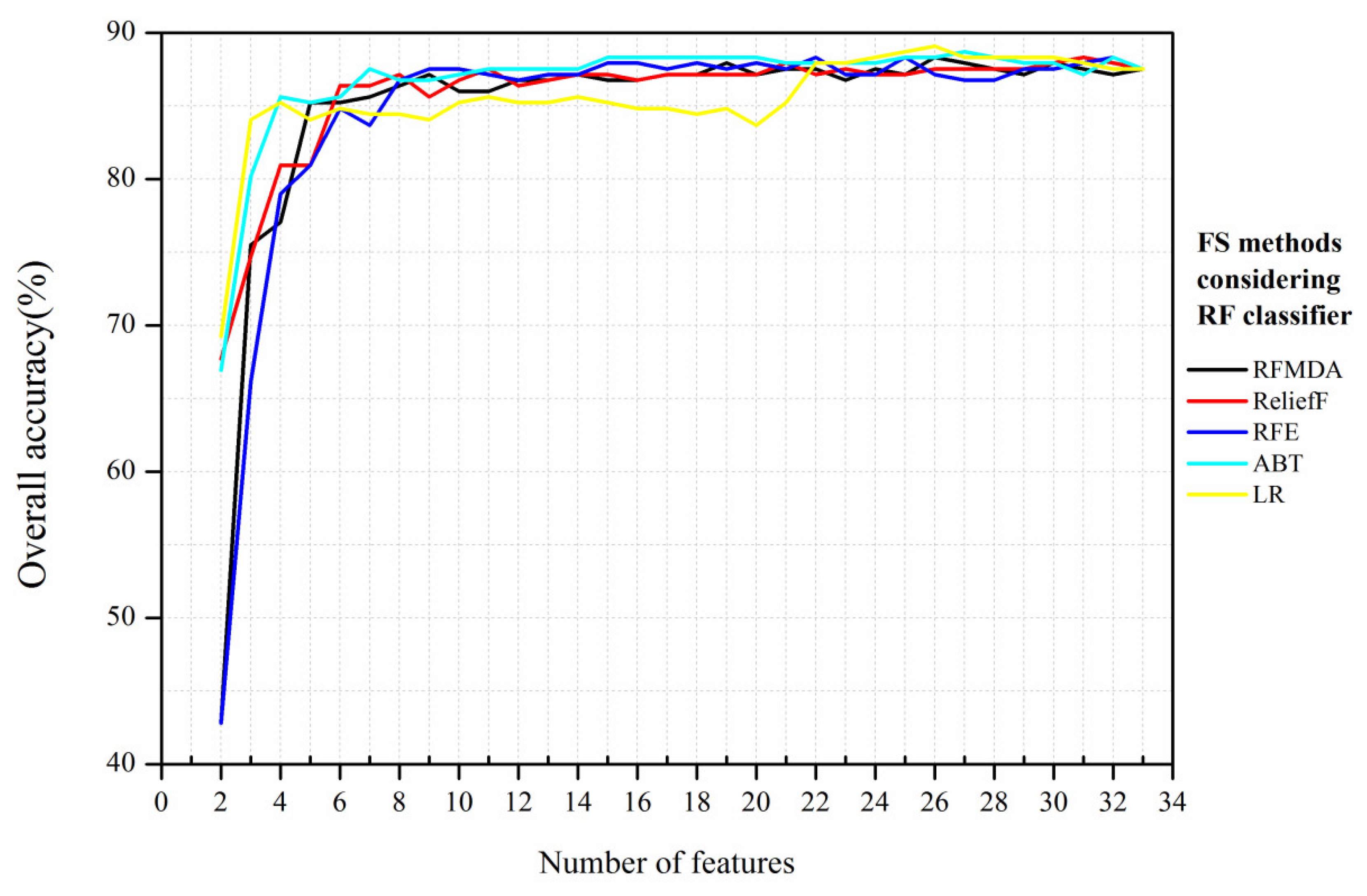
Figure 8 show the change patterns of OA using various FS methods and machine learning algorithms. In general, the OA of each classifier increased rapidly with the number of features increasing in the initial stage. When certain thresholds were reached, the curves of OA remained stable, even though more features were selected.
The RF classifier produced no significant changes in OA after the number of features exceeded 5 (Figure 5), regardless of the FS method used. This may indicate that the RF classifier is a robust algorithm that is insensitive to the addition of redundant and irrelevant features [16,18]. Here, LR had a higher classification accuracy (89.1%, 26 features) than the other FS methods (Table 7). However, the OA between 7 and 21 in LR was lower than that of the other four FS methods. The OAs of RFMDA and ReliefF were virtually the same between 12 and 22 features. For ABT, the OA value achieved 85.6% using only four features, and remained almost stable subsequently.
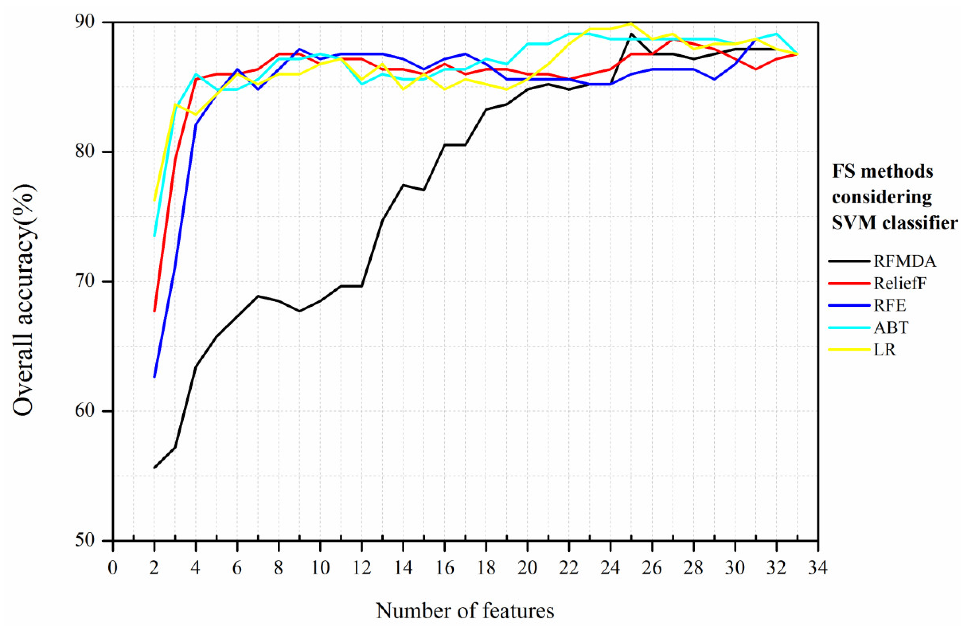
Compared with the RF classifier, the SVM classifier indicated slightly greater sensitivity to high dimensionality but this advantage was not significant. Notably, the LR method achieved the highest OA (89.88%) with 25 features, which was the maximum accuracy in all classification combinations with five FS methods and four machine learning classifiers. The curve obtained from the RFMDA method was quite different from the other FS methods; in general, OA increased steadily as features were added (Figure 6). Importantly, the RFMDA reached a maximum value (89.11%) with 25 features, and the result was approximate to that acquired by the LR method. As shown in Table 7, using ABT and LR, there were statistically significant differences (p < 0.05) compared with applying all features.
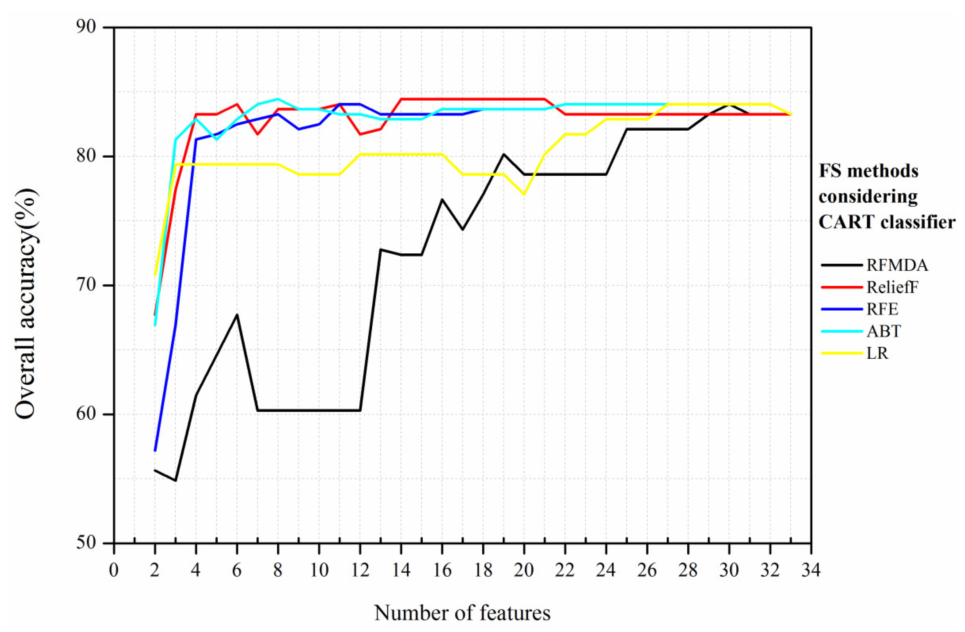
For the CART classifier, the highest OA (84.43%) was achieved with ABT and eight features, forming a parsimonious classification model because it needed the minimum number of features. Figure 7 shows that ABT, ReliefF, and RFE had almost the same curve between 14 and 22 features. For LR, the OA showed no obvious variations between 3 and 19 features. Apart from RFMDA, the remaining four FS methods presented relatively high OA accuracy (>80%) when there were more than three input features. The curve of RFMDA fluctuated greatly, indicating that dimensionality reduction did not cause the OA to increase. This may be because the important features that suit the CART classifier were eliminated.
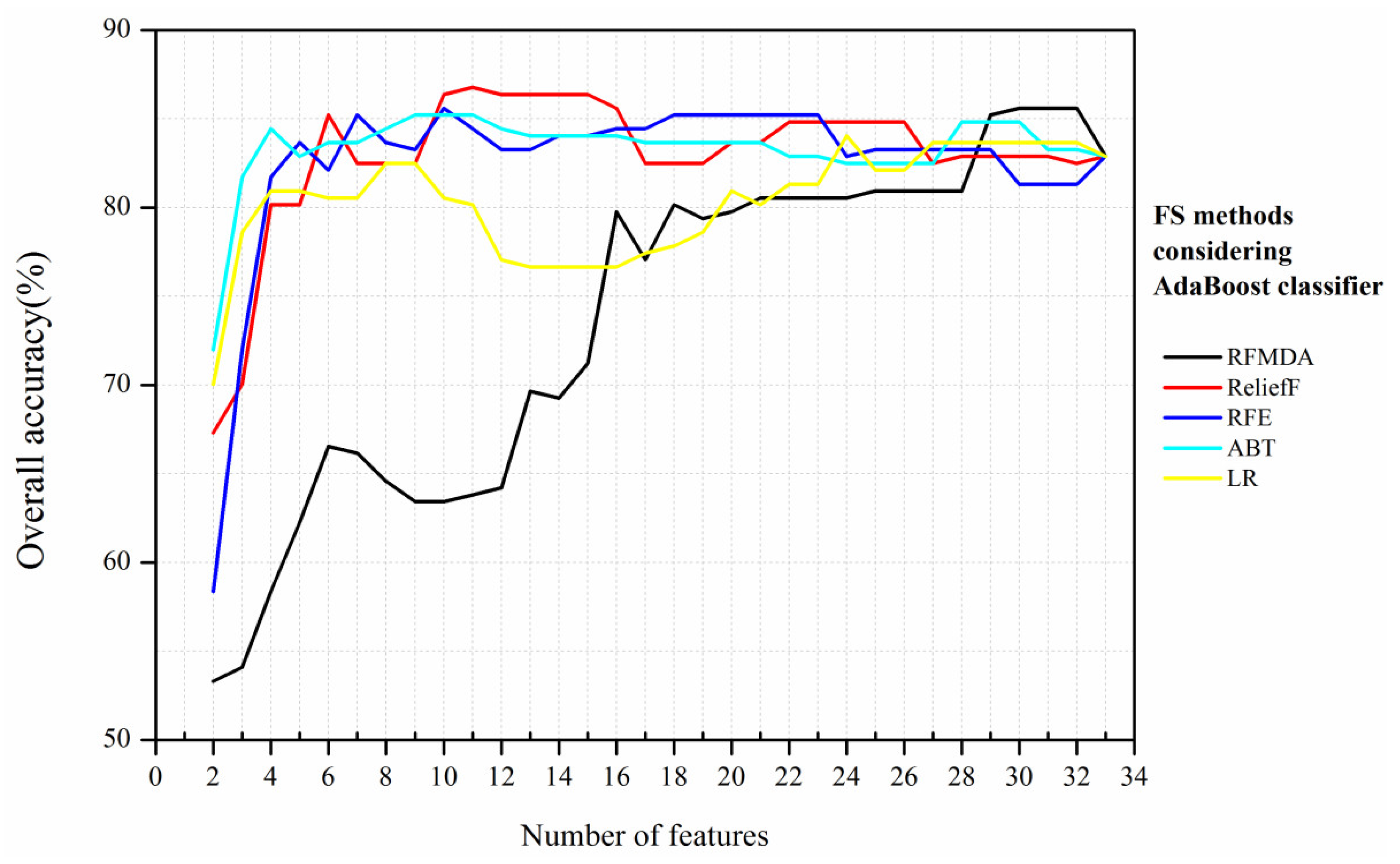
For the AdaBoost classifier, the ReliefF method obtained the best classification accuracy (86.77%) with 11 features. Moreover, ReliefF produced a ~4% improvement in OA compared with that containing all feature variables, and McNemar’s test indicated that the variation was statistically significant (p < 0.05) (Table 7). These findings show that FS is quite useful for the AdaBoost classifier. Figure 8 shows a clear fluctuation in the OA curves with the AdaBoost classifier regardless of the FS method. In addition, RFMDA and RFE showed the same maximum classification accuracy (85.6%); however, RFE required fewer features than RFMDA to achieve the same value.

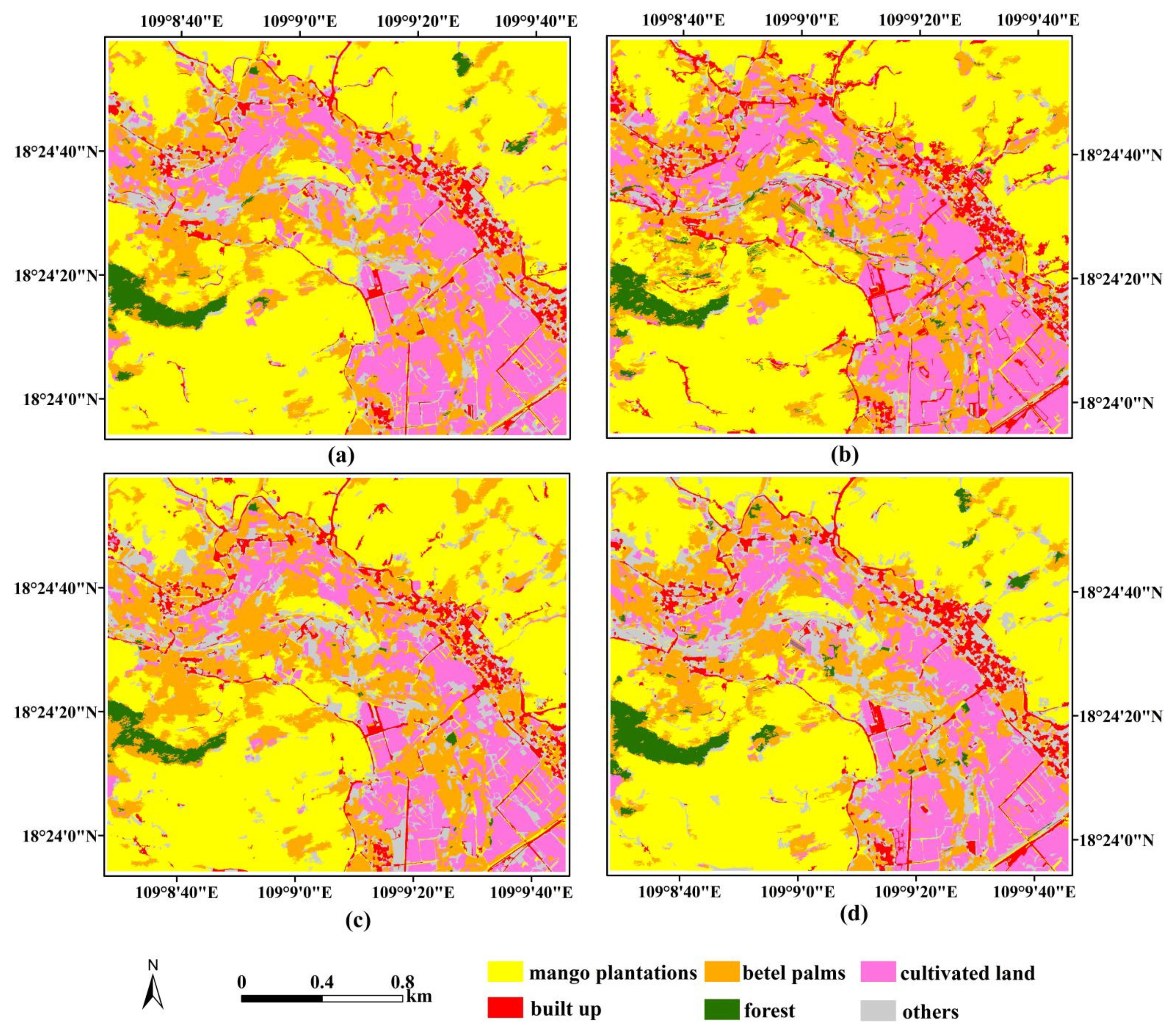
4.3. Classification Results

For a further specific analysis, we mainly compared classification accuracies of different classes based on the four machine learning algorithms. It should be noted that each classifier used the corresponding optimal feature set obtained from respective most appropriate FS method (see Section 4.2). Ultimately, there were four optimal combinations: RF-LR (with 26 features), SVM-LR (with 25 features), CART-ABT (with 8 features), and AdaBoost-ReliefF (with 11 features). In general, although all four approaches produced considerable salt-and-pepper speckled noise (Figure 9), the interesting land cover types of the study region could be reasonably identified. Accuracy indicators were calculated including producer’s accuracy (PA), user’s accuracy (UA), F1 score, kappa coefficients, and overall accuracy (OA) for all six types (Table 8).
The F1 scores of mango plantations were 95.68%, 96.07%, 97.33%, and 96.69% for RF-LR, SVM-LR, CART-ABT, and AdaBoost-ReliefF, respectively. Among them, CART-ABT achieved maximum F1 score (97.33%) with only eight features. In addition, both producer’s accuracies and user’s accuracies with four combinations exceeded 90%. These results demonstrated that mango plantations can be precisely identified whether on the ground or on the map based on the four optimal combinations. When mapping the betel palms, RF-LR presented a higher F1 score (88.89%) than other classification schemes. The confusion mistakes were encountered with types such as betel palm-cultivated land. Meanwhile, RF-LR was the only scheme in which the user’s accuracy was more than 80%. Compared to the other machine learning classifiers, the SVM-LR for recognizing cultivated land and built up produced the highest classification accuracy (F1 score is 92.91% for cultivated land and 94.74% for built up). In all classification schemes, the others classes performed poor classification results, and the F1 scores were generally in the range of 50–60%, which might be induced by the similar spectral structure between others and built up. The second lowest F1 score was produced by forest, and there were some signature confusion among forest and betel palms.
Based on the visual interpretation from the classification maps, the mango plantations and betel palms were the principal tropical crops in the study region, and mango plantations were located throughout the surrounding betel palms and cultivated land (Figure 9). The classification results were close to our previous field survey data. There were slight differences in the specific depictions under different classification schemes when the same tropical crops were compared. For example, the confusion of mango plantations and forest in the northeastern corner of the study region was more apparent in machine learning classifications that utilized the RF-LR and AdaBoost-ReliefF methods when compared with classifications using other approaches. However, the maps based on the two aforementioned approaches produced fewer jagged edges along narrow forest areas in the southeastern corner of the study region. The RF-LR method produced a more accurate visual depiction of betel palms than any classification approaches, although there remained some misclassification among forest and cultivated land and betel palm regions because of the similar spectral characteristics [30]. Moreover, the boundary between betel palms and built-up land was not well distinguished for all classification schemes.

5. Discussion

5.1. The Performance of Different Machine Learning Algorithms

Overall, the classifiers of RF and SVM showed better results than others for tropical areas object-oriented classification. However, the OA values of both RF and SVM were 87.55% without using any FS methods, which was about 5% larger than Adaboost with all 32 features. This finding further demonstrated that machine learning algorithms of RF and SVM can show a good performance in mapping betel palms and mango plantations. In addition, RF required more features than SVM to achieve maximum accuracy, which was attributed to SVM’s strengths for performing higher accuracy using limited input features [8,18]. We also found that the SVM classifier was more sensitive to the influence of data redundancy compared with the RF classifier. Ma et al. [19] also demonstrated that the Hughes effect could easily occur in SVM classifier in object-oriented classification with limitation training samples. The AdaBoost approach had the lowest OA value (82.88%) compared with classification classifiers with a full feature set, whereas the maximum accuracy achieved 86.77% with only 11 features, which was approximate to the OA obtained by the RF or SVM classifier using all features (Table 7). This indicates that AdaBoost could achieve a better classification performance using an ensemble classifier by assembling many weak classifiers into a strong classifier, especially after feature ranking selection [64,65].

5.2. The Combinations of FS Methods and Machine Learning Classifiers

The results of this study confirmed that the FS method was vitally important for depicting land cover types based on different machine learning algorithms, which supported the findings of several previous studies [18,55]. A robust FS method should be able to rank and reduce a potentially large amounts of input features [17]. In the present paper, the five FS methods evaluated in this research have their respective advantages and disadvantages with different classifiers. In general, LR was best suited to RF and SVM classifiers in this study, with an almost 2% increase in OA values, because the LR method requires fewer restrictive statistical assumptions about features (such as normally distributed or linear) compared with ordinary least squares regression [51]. Meanwhile, ABT produced relatively higher OA values using fewer features when the CART was used in classifying betel palms and mango plantations. The ABT approach overcame the relatively weak prediction capacity of depicting large trees. Furthermore, higher accuracy was performed by ABT than that of other intensive computationally methods such as RFMDA, which supports the findings of previous research [66]. ReliefF, an optimal local learning filter method, overperformed in the AdaBoost classifier because of its effectiveness and simplicity [67]. In addition, ReliefF also maintained good classification accuracy with other classifiers. Cehovin and Bosnic [41] compared ReliefF and RFMAD to select optimal features and they also found that ReliefF presented better classification accuracy, supporting our findings for the same two FS methods.
In terms of selected features, the spectral layer values and geometry have a significant advantage, but the textural features and vegetation indexes should not be ignored. There were few textural features (about 20 percent of total chosen textures) selected ultimately for mapping betel palms and mango plantations (Table 3). This demonstrated that most of the textures might be significantly correlated. As Ma et al. [68] pointed out, the number of texture features needed to be controlled considering the classification accuracy and computer times in oriented-object image analysis, especially in large regions. According to Table 5, the textural measures of GLDV entropy and GLDV angular second moment_green should be explored more closely in order to classify betel palms and mango plantations. Furthermore, GI was a very important vegetation index selected frequently for every FS method in our study.

5.3. Thematic Maps of Different Tropical Crops

In the process of tropical cropland classification, one of the greatest challenges was to identify betel palms from other class types. For all classification strategies, the UA values of betel palms were lower than those of other land cover types. Even with different FS methods, the maximum UA value of betel palms was 86.67% using RF-LR (with 26 features) and the minimum UA value of betel palms was only 73.24% using CART-ABT (with 8 features) (Table 8). A visual inspection of this study area based on field survey data showed that many betel palms were planted around built-up areas (Figure 10a,b). Normally, the height and canopy of mature betel palms can reach 10–20 and 2.5–3 m [20], respectively. The crowns of betel palms form shadows on built-up regions, causing misclassification between the two classes. Similar results of mapping vegetation areas were found in other regions using Gaofen-2 imagery [15]. In addition, betel palms were easily confused with neighboring forest and cultivated land (Figure 10c), which was attributed to the spatial complexity of tropical agricultural planting regions. This was also demonstrated earlier in the analysis of classification accuracy (Section 4.3). When performing the segmentation process in objected-based image analysis, betel palm regions may be merged with adjacent forest or cultivated land because of the similar spectral characteristics to these land-use types. Wang et al. [69] also pointed out that a mixed object is more obvious along the edge or borders of different types. Although the influence of over-segmentation and under-segmentation can be reduced to some extent using the ancillary features, the classification accuracy of betel palms will still be inevitably affected. Surprisingly, we obtained a relatively satisfactory classification accuracy of mango plantations; this is because Gaofen-2 imagery uses sub-meter resolution data and has more abundant spatial and structure information. As a typical tropical crop, evergreen mango trees need enough sunlight for photosynthesis. Therefore, mango plantations usually exhibit bigger planting spacing in the rows (3–4 m) (Figure 10d). Compared to other tropical vegetation, the rounded canopies of mango trees show a lower and looser characteristic. Due to this distribution, mango plantations had unique textural patterns in Gaofen-2 imagery that can overcome the spectral similarity between mango plantations and other tropical vegetation. Leckie and Gillis [70] pointed out that VHR imagery can replace the aerial photography in the field of land cover mapping. In this paper, we similarly found that Gaofen-2 imagery performed brilliantly in tropical crop classification.
Usually, classification accuracy (including OA, F1 score, user’s accuracy, and producer’s accuracy) is used to evaluate the optimal combinations of FS methods and classifiers. However, to obtain higher classification results, more evaluation criteria should be considered, such as efficiency and processing times. When the difference of classification accuracy is small, processing times may be more important to big study areas, especially for mapping with high-resolution images [17]. In future research, varying the method of accuracy evaluation should be implemented to evaluate the tradeoff between accuracy and efficiency. About the machine learning approach, we just explored the performance of conventional classifiers. To improve the classification accuracy for recognizing tropical crops, the state-of-the-art classification technique (e.g., deep learning methods) should be applied in our following studies. In addition, this paper only focused on the optical image in mapping two tropical crops. Nevertheless, the high frequency of cloud coverage makes it very difficult to acquire high-quality optical data in tropical regions [71]. Considering the demand for periodic recognition, more cloud-free data (such as synthetic aperture radar image (SAR)) are required for mapping tropical crops in our following study.

6. Conclusions

Mapping of tropical agricultural land cover types is incredibly difficult due to their complexity and heterogeneity in finer resolution imagery. In this study, our specific objectives were to assess the appropriate combinations of FS methods and machine learning classifiers, and evaluate the capability of sub-meter resolution Gaofen-2 imagery for identifying betel palms and mango plantations based on object-oriented classification. The SVM and RF classifiers based exclusively on classification accuracy results showed a slight advantage for the purposes of mapping tropical crops relative to the other machine learning classifiers. Furthermore, we also found that all classifiers presented better performance after FS methods were used to choose the optimal subsets of features. Compared with classification results without the FS method, different classifiers with an optimal features subset could increase the overall accuracy by 1–4%. Moreover, different FS methods showed adaptability to various machine learning classifiers. In general, RF and SVM classifiers applying the LR method showed higher overall accuracies. For the CART classifier, ABT was identified as the most suitable FS method for identifying tropical crops. The AdaBoost classifier with ReliefF was also a suitable option for classifying tropical crops under a comprehensive consideration of classification precision and computation time. When evaluating classification results based both on the ground and on the map, this study indicated that all four optimal combinations of FS methods and classifiers could correctly recognize mango plantation regions, whereas betel palms were best depicted by using the RF-LR method with 26 features. Even though the classification accuracy of AdaBoost-ReliefF was not the highest, we suggested it was a practical scheme if identifying betel palms and mango plantations in large study regions.
Our research confirmed the utility of Gaofen-2 for mapping betel palms and mango plantations in complex tropical agricultural regions with heterogeneous planting structure and a high degree of fragmentation. These findings provide an effective technical approach for accurate tropical crop identification, which is the foundation for tropical agricultural regional planning and management.

Author Contributions

All authors contributed equally to the design of the research. H.L. (Hongxia Luo) conducted the field work and prepared the origin manuscript. M.L. and S.D. revised the manuscript and processed the Gaofen-2 imagery. H.L. (Hailiang Li) and J.F. designed the programming of R codes. Y.L., Y.H., Q.Z., and X.Y. collected the field samples. All authors have read and agreed to the published version of the manuscript.

Funding

This study was funded by the Natural Science Foundation of Hainan, China (grant numbers 620MS86, 619MS100); the Central Public-interest Scientific Institution Basal Research Fund for the Chinese Academy of Tropical Agricultural Sciences (grant number 1630072017004); the key R&D programme of Hainan Province (grant number ZDYF2021GXJS215); and the Hainan Provincial Key Laboratory of Practical Research on Tropical Crops Information Technology, China (grant numbers RDZWKFJJ2019001, XXS-201903).

Institutional Review Board Statement

Not applicable.

Informed Consent Statement

Not applicable.

Data Availability Statement

The Gaofen-2 product can be obtained at http://www.cresda.com/CN/ (accessed on 5 March 2020).

Acknowledgments

We also thank the reviewers and editors for the suggestions and comments for improving the manuscript.

Conflicts of Interest

The authors declare no conflict of interest.

References

  1. Phalke, A.; Ozdogan, M. Large area cropland extent mapping with Landsat data and a generalized classifier. Remote Sens. Environ. 2018, 219, 180–195. [Google Scholar] [CrossRef]
  2. Sanches, I.D.; Feitosa, R.Q. Campo verde database: Seeking to improve agricultural remote sensing of tropical areas. IEEE Geosci. Remote Sens. Lett. 2018, 15, 369–373. [Google Scholar] [CrossRef]
  3. Wardlow, B.D.; Egbert, S.L. Large-area crop mapping using time-series MODIS 250m NDVI data: An assessment for the U.S. central great plains. Remote Sens. Environ. 2008, 112, 1096–1116. [Google Scholar] [CrossRef]
  4. Immitzer, M.; Vuolo, F.; Atzberger, C. First experience with Sentinel-2 data for crop and tree species classifications in central Europe. Remote Sens. 2016, 8, 166. [Google Scholar] [CrossRef]
  5. Zhang, D.J.; Pan, Y.Z.; Zhang, J.S.; Hu, T.G.; Zhao, J.H.; Li, N.; Chen, Q. A generalized approach based on convolutional neural networks for large area cropland mapping at very high resolution. Remote Sens. Environ. 2020, 247, 111912. [Google Scholar] [CrossRef]
  6. Zhang, P.; Hu, S.G.; Li, W.D.; Zhang, C.R. Parcel-level mapping of crops in a smallholder agricultural area: A case of central China using single-temporal VHSR imagery. Comput. Electron. Agric. 2020, 175, 105581. [Google Scholar] [CrossRef]
  7. Duro, D.C.; Franklin, S.E.; Dube, M.G. A comparison of pixel-based and object-based image with selected machine learning algorithms for the classification of agricultural landscapes using SPOT-5 HRG imagery. Remote Sens. Environ. 2012, 118, 259–272. [Google Scholar] [CrossRef]
  8. Ghosh, A.; Joshi, P. A comparison of selected classification algorithms for mapping bamboo patches in lower Gangetic plains using very high resolution Worldview 2 imagery. Int. J. Appl. Earth Obs. 2014, 26, 298–331. [Google Scholar] [CrossRef]
  9. Li, D.; Ke, Y.H.; Gong, H.L.; Li, X.J. Object-Based urban tree species classification using bi-temporal Worldview-2 and worldview-3 images. Remote Sens. 2015, 7, 16917–16937. [Google Scholar] [CrossRef] [Green Version]
  10. Bofana, J.; Zhang, M.; Nabil, M.; Wu, B.F.; Tian, F.Y.; Liu, W.J.; Zeng, H.W.; Zhang, N.; Nangombe, S.; Cipriano, S.; et al. Comparison of Dierent Cropland Classification Methods under Diversified Agroecological Conditions in the Zambezi River Basin. Remote Sens. 2020, 12, 2096. [Google Scholar] [CrossRef]
  11. Tarantino, E.; Figorito, B. Mapping Rural Area with widespread plastic covered vineyards true color aerial data. Remote Sens. 2012, 4, 1913–1928. [Google Scholar] [CrossRef] [Green Version]
  12. Han, H.B.; Ma, M.G.; Wang, X.F.; Ma, S.C. Classifying cropping area of middle Heihe River Basin in China using multitemporal normalized difference vegetation index data. J. Appl. Remote Sens. 2018, 8, 083654. [Google Scholar] [CrossRef]
  13. Puissant, A.; Rougier, S.; Stumpf, A. Object-oriented mapping of urban trees using random forest classifiers. Int. J. Appl. Earth Obs. 2014, 26, 235–245. [Google Scholar] [CrossRef]
  14. Zhu, Z.; Gallant, A.L.; Woodcock, C.E.; Pengra, B.; Olofsson, P.; Loveland, T.R.; Jin, S.M.; Dahal, D.; Yang, L.M.; Auch, R.F. Optimizing selection of training and auxiliary data for operational land cover classification for the LCMAP initiative. ISPRS J. Photogramm. 2016, 122, 206–221. [Google Scholar] [CrossRef] [Green Version]
  15. Wang, H.; Wang, C.B.; Wu, H.G. Using GF-2 imagery and the conditional random field model for urban forest cover mapping. Remote Sens. Lett. 2016, 7, 378–387. [Google Scholar] [CrossRef]
  16. Stefanos, G.; Tais, G.; Sabine, V.; Moritz, L.; Michal, S.; Stamatis, K.; Eleonore, W. Less is more: Optimizing classification performance through feature selection in a very-high-resolution remote sensing object-based urban application. GISci Remote Sens. 2017, 55, 221–242. [Google Scholar]
  17. Laliberte, A.S.; Browning, D.M.; Rango, A. A comparison of three feature selection methods for object-based classification of sub-decimeter resolution UltraCam-L imagery. Int. J. Appl. Earth Obs. 2012, 15, 70–78. [Google Scholar] [CrossRef]
  18. Cánovas-García, F.; Alonso-Sarría, F. Optimal Combination of Classification Algorithms and Feature Ranking Methods for Object-Based Classification of Submeter Resolution Z/I-Imaging DMC Imagery. Remote Sens. 2015, 7, 4651–4677. [Google Scholar] [CrossRef] [Green Version]
  19. Ma, L.; Fu, T.Y.; Blaschke, T.; Li, M.C.; Tiede, D.; Zhou, Z.J.; Ma, X.X.; Chen, D.L. Evaluation of feature selection methods for object-Based land cover mapping of unmanned aerial vehicle imagery using random forest and support vector machine classifiers. ISPRS Int. J. Geo-Inf. 2017, 6, 51. [Google Scholar] [CrossRef]
  20. Staples, G.W.; Bevacqua, R.F. Areca catechu (betel nut palm). Species Profiles Pac. Isl. Agrofor. 2006, 13, 1–17. [Google Scholar]
  21. NBSH (National Bureau of Statistics of Hainan). Hainan Statistical Yearbook 2017; China Statistics Press: Beijing, China, 2020. (In Chinese) [Google Scholar]
  22. Cheng, J.D.; Lin, J.P.; Lu, S.Y.; Huang, L.S.; Wu, H.L. Hydrological characteristics of betel nut plantations on slopelands in central Taiwan/ Caracteristiques hydrologiques de plantations de noix de betel sur des versants du centre Taiwan. Hydrol. Sci. J. 2008, 53, 1208–1220. [Google Scholar] [CrossRef]
  23. Rosa, L.E.C.L.; Feitosa, R.Q.; Happ, P.N.; Sanches, I.D.; Costa, G.A.O.P. Combining deep learning and prior knowledge for crop mapping in tropical regions from multitemporal SAR Image Sequences. Remote Sens. 2019, 11, 2029. [Google Scholar] [CrossRef] [Green Version]
  24. Chen, B.Q.; Li, X.P.; Xiao, X.M.; Zhao, B.; Dong, J.W.; Kou, W.L.; Qin, Y.W.; Yang, C.; Wu, Z.X.; Sun, R.; et al. Mapping tropical forests and rubber deciduous plantations in Hainan Island, China by intergrating PALSAR 25-m and multi-temporal Landsat images. Int. J. App. Earth Obs. 2016, 50, 117–130. [Google Scholar] [CrossRef]
  25. Chen, C.Y.; Jing, L.H. Stand species identification using GF-2 imagery and airborne LiDAR data based on SVM classifier. IOP Conf. Ser. Earth Environ. Sci. 2020, 502, 012045. [Google Scholar] [CrossRef]
  26. Wu, Q.; Zhong, R.F.; Zhao, W.J.; Song, K.; Du, L.M. Land-cover classification using GF-2 images and airborne lidar data based on random forest. Int. J. Remote Sens. 2019, 40, 2410–2426. [Google Scholar] [CrossRef]
  27. Tong, X.Y.; Xia, G.S.; Lu, Q.K.; Shen, H.F.; Li, S.Y.; You, S.C.; Zhang, L.P. Land-cover classification with high-resolution remote sensing images using transferable deep models. Remote Sens. 2020, 237, 111322. [Google Scholar] [CrossRef] [Green Version]
  28. Cooley, T.; Anderson, G.P.; Felde, G.W.; Hoke, M.L.; Ratkowski, A.J.; Chetwynd, J.H.; Gardner, J.A.; Adler-Golden, S.M.; MatthewMW, B.; Bernstein, L.S. FLAASH, a MODTRAN4-based atmospheric correction algorithm, its application and validation. In Proceedings of the 2002 IEEE International Geoscience and Remote Sensing Symposium & 24th Canadian Symposium on Remote Sensing, Toronto, Canada, 24–28 June 2002. [Google Scholar]
  29. Wang, T.; Zhang, H.S.; Lin, H.; Fang, C.Y. Textural-spectral feature-based species classification of mangroves in Mai Po Nature reserve from Worldview-3 imagery. Remote Sens. 2016, 8, 24. [Google Scholar] [CrossRef] [Green Version]
  30. Luo, H.X.; Dai, S.P.; Li, M.F.; Liu, E.P.; Zheng, Q.; Hu, Y.Y.; Yi, X.P. Comparison of machine learning algorithms for mapping mango plantations based on Gaofen-1 imagery. J. Integr. Agric. 2020, 19, 2815–2828. [Google Scholar] [CrossRef]
  31. Congalton, R.C. A review of assessing the accuracy of classifications of remotely sensed data. Remote Sens. Environ. 1991, 37, 35–46. [Google Scholar] [CrossRef]
  32. Jia, K.; Tu, Y.X.; Li, Q.Z.; Yao, Y.J. Land use and land cover classification using Chinese GF-2 multispectral data in a region of the north China plain. Front. Earth Sci. 2019, 13, 327–335. [Google Scholar] [CrossRef]
  33. Dragut, L.; Tiede, D.; Levick, S.R. ESP: A tool to estimate scale parameter for multiresolution image segmentation of remotely sensed data. Int. J. Geogr. Inf. Sci. 2010, 24, 859–871. [Google Scholar] [CrossRef]
  34. Baatz, M.; Schape, A. Multiresolution segmentation: An optimization approach for high quality multi-scale image segmentation. In Proceedings of the Angewandte Geographische Informations verarbeitung XII, Beiträge zum AGIT Symposium, Karlsruhe, Germany, 1 January 2000. [Google Scholar]
  35. Myint, S.W.; Gober, P.; Brazel, A.; Grossman-Clarke, S.; Weng, Q. Per-pixel vs: Object-based classification of urban land cover extraction using high spatial resolution imagery. Remote Sens. Environ. 2011, 115, 1145–1161. [Google Scholar] [CrossRef]
  36. Haralick, R.M.; Shanmugam, K.S. Combined spectral and spatial processing of ERTS imagery data. Remote Sens. Environ. 1974, 3, 3–13. [Google Scholar] [CrossRef] [Green Version]
  37. Ke, Y.H.; Quackenbush, L.; Im, J. Synergistic use of QuickBird multispectral imagery and LIDAR data for object-based forest species classification. Remote Sens. Environ. 2010, 114, 1141–1154. [Google Scholar] [CrossRef]
  38. Peña-Barragán, J.M.; Ngugi, M.K.; Plant, R.E.; Six, J. Object-based crop identification using multiple vegetation indices, textural features and crop phenology. Remote Sens. Environ. 2011, 115, 1301–1316. [Google Scholar] [CrossRef]
  39. Huang, Y.H.; Zhao, C.P.; Yang, H.J.; Song, X.Y.; Chen, J.; Li, Z.H. Feature selection solution with high dimensionality and low sample size for land classification in object-based image analysis. Remote Sens. 2017, 9, 939. [Google Scholar] [CrossRef] [Green Version]
  40. Li, C.C.; Wang, J.; Wang, L.; Hu, L.Y.; Gong, P. Comparison of classification algorithms and training samples sizes in urban land classification with landsat thematic mapper imagery. Remote Sens. 2014, 6, 964–983. [Google Scholar] [CrossRef] [Green Version]
  41. Cehovin, L.; Bosnic, Z. Empirical evaluation of feature selection methods in classification. Intell. Data Anal. 2010, 14, 265–281. [Google Scholar] [CrossRef] [Green Version]
  42. Huang, P.; Li, Y.P.; Lv, X.Y.; Chen, W.; Liu, S.X. Recognition of common non-normal walking actions based on Relief-F feature selection and relief-bagging-SVM. Sensors 2020, 20, 1447. [Google Scholar] [CrossRef] [Green Version]
  43. Li, D.Y.; Wen, G.H.; Hou, Z.; Huan, E.Y.; Hu, Y.; Li, H.Z. RTC Relief-F: An effective clustering and ordering-based ensemble pruning algorithm for facial expression recognition. Knowl. Inf. Syst. 2019, 59, 219–250. [Google Scholar] [CrossRef]
  44. Wang, C.B.; Pan, Y.P.; Chen, J.G.; Ouyang, Y.P.; Rao, J.F.; Jiang, Q.B. Indicator element selection and geochemical anomaly mapping using recursive feature elimination and random forest methods in the Jingdezhen region of Jiangxi Province, south China. Appl. Geochem. 2020, 122, 104760. [Google Scholar] [CrossRef]
  45. You, W.J.; Yang, Z.J.; Ji, G.L. Feature selection for high dimensional multi-category data using PLS-based local recursive feature elimination. Expert Syst. Appl. 2014, 41, 1463–1475. [Google Scholar] [CrossRef]
  46. Verikas, A.; Gelzinis, A.; Bacauskiene, M. Mining data with random forest: A survey and results of new tests. Pattern Recogn. 2011, 44, 330–349. [Google Scholar] [CrossRef]
  47. Ge, Y.; He, J.Z.; Zhu, Y.G.; Zhang, J.B.; Xu, Z.H.; Zhang, L.M.; Zheng, Y.M. Differences in soil bacterial diversity driven by contemporary disturbances or historical contingencies? Multidiscip. J. Microb. Ecol. 2008, 2, 254–264. [Google Scholar] [CrossRef] [Green Version]
  48. Friedman, J.H. Greedy function approximation: A gradient boosting machine. Ann. Stat. 2001, 29, 1189–1232. [Google Scholar] [CrossRef]
  49. Zhao, F.J.; Liu, J.T.; Qu, X.C.; Xu, X.H.; Chen, X.L.; Yang, X.; Cao, F.; Liang, J.M.; Tian, J. In vivo quantitative evaluation of vascular parameters for angiogenesis based on sparse principal component analysis and aggregated boosted trees. Inst. Phys. Eng. Med. 2014, 59, 7777–7791. [Google Scholar]
  50. Kakade, A.; Kumari, B.; Dholaniya, P.S. Feature selection using logistic regression in case-control DNA methylation data of Parkinson’s disease: A comparative study. J. Theorl Biol. 2018, 457, 14–18. [Google Scholar] [CrossRef]
  51. Cheng, Q.; Varshney, P.K.; Arora, M. Logistic regression for feature selection and soft classification of remote sensing data. IEEE Geosci Remote Sens. 2006, 3, 491–494. [Google Scholar] [CrossRef]
  52. Breiman, L. Bagging predictors. Mach. Learn. 1996, 26, 123–140. [Google Scholar] [CrossRef] [Green Version]
  53. Noi, P.T.; Kappas, M. Comparison of random forest, k-Nearest neighbor, and support vector machine classifiers for land cover classification using Sentinel-2 imagery. Sensors 2018, 18, 18. [Google Scholar]
  54. Vapnik, V.N.; Chervonenkis, A.Y. On the uniform convergence of relative frequencies of events to their probabilities. Theor. Probab. Appl. 1971, 16, 264–280. [Google Scholar] [CrossRef]
  55. Pal, M. Random forest classifier for remote sensing classification. Int. J. Remote Sens. 2005, 26, 217–222. [Google Scholar] [CrossRef]
  56. Breiman, L.; Friedman, J.H.; Olshen, R.A.; Stone, C.J. Classification and Regression Trees (CART). Biometrics 1984, 40, 358. [Google Scholar]
  57. Bashir, S.; Qamar, U.; Khan, F.H.; Javed, M.Y. An efficient rule-based classification of diabetes using ID3, C4.5 & CART ensembles. In Proceedings of the 12th International conference on Frontiers of Information Technology, Islamabad, Pakistan, 17–19 December 2014. [Google Scholar]
  58. Freund, Y.; Schapire, R.E. Experiments with a new boosting algorithm. In Proceedings of the Machine Learning: Proceedings of the Thirteenth International Conference, Bari, Italy, 3–6 July 1996. [Google Scholar]
  59. Tsutsumida, N.; Comber, A.J. Measures of spatio-temporal accuracy for time series land cover data. Int. J. Appl. Earth Obs. 2015, 41, 46–55. [Google Scholar] [CrossRef]
  60. Verma, A.K.; Garg, P.K.; Prasad, K.S. Sugarcane crop identification from LISS IV data using ISODATA, MLC, and indices based decision tree approach. Arab J. Geosci. 2017, 10, 1–17. [Google Scholar]
  61. Zurqani, H.A.; Post, C.J.; Mikhailova, E.A.; Cope, M.P.; Allen, J.S.; Lytle, B.A. Evaluating the integrity of forested riparian buffers over a large area using LiDAR data and google earth engine. Sci. Rep. 2020, 10, 14096. [Google Scholar] [CrossRef]
  62. Chuang, M.Y.; Shiu, Y.S. A comparative analysis of machine learning with WorldView-2 pan-sharpened imagery for tea crop mapping. Sensors 2016, 16, 594–617. [Google Scholar] [CrossRef] [Green Version]
  63. Gheyas, I.A.; Smith, L.S. Feature subset selection in large dimensionality domains. Pattern Recogn. 2010, 43, 5–13. [Google Scholar] [CrossRef] [Green Version]
  64. Li, M.C.; Ma, L.; Blaschke, T.; Cheng, L.; Tiede, D. A systematic comparison of different object-based classification techniques using high spatial resolution imagery in agricultural environments. Int. J. Appl. Earth Obs. 2016, 49, 87–98. [Google Scholar] [CrossRef]
  65. Hu, G.; Yin, C.J.; Wan, M.Z.; Zhang, Y.; Fang, Y. Recognition of diseased pinus trees in UAV images using deep learning and AdaBoost classifier. Biosyst. Eng. 2020, 194, 138–151. [Google Scholar]
  66. De’ath, G. Boosted trees for ecological modeling and prediction. Ecology 2007, 88, 243–251. [Google Scholar] [CrossRef]
  67. Sun, Y.J. Iterative RELIEF for Feature Weighting: Algorithms, Theories, and Applications. IEEE Trans. Pattern Anal. 2007, 29, 1035–1051. [Google Scholar] [CrossRef]
  68. Ma, L.; Cheng, L.; Li, M.C.; Liu, Y.X.; Ma, X.X. Training set size, scale, and features in geographic object-based image analysis of very high resolution unmanned aerial vehicle imagery. ISPRS J. Photogramm. 2015, 102, 14–27. [Google Scholar] [CrossRef]
  69. Wang, L.; Sousa, W.P.; Gong, P. Integration of object-based and pixel-based classification for mapping mangroves with IKONOS imagery. Int. J. Remote Sens. 2004, 25, 5655–5668. [Google Scholar] [CrossRef]
  70. Leckie, D.; Gillis, M. Forest inventory in Canada with an emphasis on map production. Forest Chron. 1995, 71, 74–88. [Google Scholar] [CrossRef]
  71. Dong, J.W.; Xiao, X.M.; Chen, B.Q.; Torbick, N.; Jin, C.; Zhang, G.L.; Biradar, C. Mapping deciduous rubber plantations through integration of PALSAR and multi-temporal Landsar imagery. Remote Sens. Environ. 2013, 134, 392–402. [Google Scholar] [CrossRef]
Figure 1. The study area location. (a) The DEM of Hainan. (b) The study region, located in the southwestern Sanya city, China. (c) Gaofen-2 imagery composed of band 3, 2, and 1 (red, green, and blue bands, respectively).
Remotesensing 14 01757 g001
Figure 2. The workflow for object-oriented tropical crop classification (betel palms and mango plantations).
Remotesensing 14 01757 g002
Figure 3. Image segmentation at scale parameter 95. The detail larger versions can be seen in Figure 4.
Remotesensing 14 01757 g003
Figure 4. The larger versions of respective four red blocks (ad) in Figure 3.
Remotesensing 14 01757 g004
Figure 5. Relationships among overall accuracy and the number of features based on random forest (RF) classifier. RFMDA, RFE, ABT, and LR are the abbreviations of random forest mean decrease in accuracy, recursive feature elimination, aggregated boosted tree, and logistic regression, respectively.
Remotesensing 14 01757 g005
Figure 6. Relationships among overall accuracy and the number of features based on support vector machine (SVM) classifier. RFMDA, RFE, ABT, and LR are the abbreviations of random forest mean decrease in accuracy, recursive feature elimination, aggregated boosted tree, and logistic regression, respectively.
Remotesensing 14 01757 g006
Figure 7. Relationships among overall accuracy and the number of features based on classification and regression tree (CART) classifier. RFMDA, RFE, ABT, and LR are the abbreviations of random forest mean decrease in accuracy, recursive feature elimination, aggregated boosted tree, and logistic regression, respectively.
Remotesensing 14 01757 g007
Figure 8. Relationships among overall accuracy and the number of features based on AdaBoost classifier. RFMDA, RFE, ABT, and LR are the abbreviations of random forest mean decrease in accuracy, recursive feature elimination, aggregated boosted tree, and logistic regression, respectively.
Remotesensing 14 01757 g008
Figure 9. Classification maps produced by different machine learning classifiers with the optimal combination of FS methods for (a) RF-LR with 26 features, (b) SVM-LR with 25 features, (c) CART-ABT with 8 features, and (d) AdaBoost-ReliefF with 11 features.
Remotesensing 14 01757 g009
Figure 10. Field photos illustrating different classification types in parts of study area. (a) Gaofen-2 imagery in a part of study area. the three blocks (c, b, and d) are parts of Figure 10a, and the detail field photos are shown as follows: (b) betel palms, (c) betel palms planting neighboring cultivated land, and (d) mango plantations.
Remotesensing 14 01757 g010
Table 1. Specifications of GF-1 satellite.
CameraSpectral Range of Four BandsSpatial ResolutionWidthRevisit Period
multispectral cameras0.45–0.52 μm4 m45 km (for two cameras together)5 days
0.52–0.59 μm
0.63–0.69 μm
0.77–0.89 μm
Panchromatic camera0.45–0.90 μm1 m
Table 2. Summary of the initial features selected.
TypesFeaturesExplanation
Layer values (10)Mean; standard deviation for blue, green, red, and near-infrared spectrum (NIR); max. diff; brightness.Layer value features calculate corresponding information based on the spectral properties of image objects.
Geometry (9)Border index, area (Px), roundness, compactness, shape index, rectangular fit, density, and asymmetry.Geometry features principally evaluate the shape of image objects.
Texture (80)Gray-level co-occurrence matrix (GLCM) homogeneity, GLCM contrast, GLCM dissimilarity, GLCM entropy, GLCM mean, GLCM correlation, GLCM variance, GLCM angular second moment, gray-level difference vector (GLDV) homogeneity, GLDV contrast, GLDV dissimilarity, GLDV entropy, GLDV mean, GLDV correlation, GLDV variance, and GLDV angular second moment.Texture features utilize texture values derived from GLCM or GLDV using blue, green, red, and NIR bands.
Vegetation index (10)Greenness index (GI), modified chlorophyll absorption in reflectance index (MCARI), modified simple ratio (MSR), green normalized difference vegetation index (GNDVI), normalized difference vegetation index (NDVI), renormalized difference vegetation index (RDVI), simple ratio index (SRI), transformed chlorophyll absorption in reflectance index (TCARI), triangular vegetation index (TVI), and green vegetation index (VIgreen)These 10 vegetation indexes are usually applied in agricultural identification because of their ability to recognize the spatial characteristics of certain crops. For detailed formulas refer to Peña-Barragán et al. [38].
Notes: Numbers in parenthesis () represent the number of each type of initial features.
Table 3. The 33 features remained based on Spearman’s rank correlation coefficient method.
TypesFeatures
Layer values (7)Mean_blue, mean_NIR (near-infrared spectrum), standard deviation_blue, standard deviation_red, standard deviation_NIR, max. diff, and brightness.
Geometry (6)Border index, area (Px), roundness, rectangular fit, density, and asymmetry.
Texture (17)Gray-level co-occurrence matrix (GLCM) entropy, gray-level difference vector (GLDV) contrast_blue, GLDV contrast_red, GLDV contrast_NIR, GLCM variance, GLCM variance_blue, GLCM variance_green, GLCM variance_red, GLCM variance_NIR, GLCM mean, GLCM angular second moment, GLCM dissimilarity_red, GLDV entropy, GLDV angular second moment_green, GLDV mean_NIR, GLCM contrast_blue, and GLCM correlation.
Vegetation index (3)Greenness index (GI), triangular vegetation index (TVI), and green vegetation index (VIgreen).
Notes: Numbers in parenthesis () represent the number of each type of selected features.
Table 4. Optimal parameters of four machine learning algorithms.
ClassifiersParametersValue
RFntree500
mtry10
SVMgamma0.001
kernelradial
C3
degree3
CARTsplitgini
cp0.01
AdaBoostmfinal50
coeflearnBreiman
Table 5. Top 15 features using various FS methods.
RFMDAReliefFRFEABTLR
GIstandard deviation_blueGIGImax. diff
VIgreenstandard deviation_redVIgreenmean_blueGI
GLDV angular second moment_greenmax. diffmean_bluestandard deviation_blueGLDV Entropy
GLDV entropyGIstandard deviation_blueGLDV entropyrectangular fit
standard deviation_blueVIgreenstandard deviation_NIRGLDV angular second moment_greenVIgreen
standard deviation_NIRGLDV entropymax. diffstandard deviation_NIRdensity
mean_blueGLCM dissimilarity_redstandard deviation_redmax. diffGLCM entropy
max. diffTVIGLDV angular second moment_greenGLCM correlationGLCM correlation
standard deviation_redGLDV contrast_redbrightnessbrightnessasymmetry
GLCM dissimilarity_redstandard deviation_NIRGLDV entropyGLCM varianceroundness
GLCM correlationmean_blueGLCM correlationGLCM dissimilarity_redGLDV mean_NIR
brightnessGLDV angular second moment_greenGLCM dissimilarity_redGLDV angular second momentGLCM dissimilarity_red
GLDV mean_NIRbrightnessTVITVIGLCM variance_red
GLCM varianceGLDV contrast_blueGLCM varianceborder indexGLCM mean
GLCM contrast_blueGLCM contrast_blueborder indexasymmetryGLCM variance_green
Table 6. Summary of different categories of features among the top 15 features according to Table 5.
FS MethodsThe Detail Description of FeaturesLayer ValuesGeometryTextureVegetation Index
RFMDANumber of features5172
The proportion of features among the top 15 features33.33%6.67%46.67%13.33%
The proportion of features among the total number of respective categories in the chosen 33 features71.43%16.67%41.18%66.67%
ReliefFNumber of features5163
The proportion of feature among the top 15 features33.33%6.67%40%20%
The proportion of features among the total number of respective categories in chosen 33 features71.43%16.67%35.29%100%
RFENumber of features6252
The proportion of features among the top 15 features40%13.33%33.33%13.33%
The proportion of features among the total number of respective categories in chosen 33 features85.71%33.33%35.29%66.67%
ABTNumber of features5262
The proportion of features among the top 15 features33.33%13.33%40%13.33%
The proportion of features among the total number of respective categories in chosen 33 features71.43%33.33%35.29%66.67%
LRNumber of features1482
The proportion of features among the top 15 features6.67%26.67%53.33%13.33%
The proportion of features among the total number of respective categories in chosen 33 features14.29%66.67%47.06%66.67%
Notes: The total number of respective categories from chosen 33 feature can be found in Table 3. Specifically, the total numbers for layer values, geometry, texture, and vegetation index were 7, 6, 17, and 3, respectively.
Table 7. Maximal OA (%) for each machine learning classifier using various FS methods.
FS MethodsRFMDAReliefFRFEABTLRAll Features
Classifiers
RF88.33 (26)88.33 (31)88.33 (22)88.72 (27)89.1 (26)87.55
SVM89.11 (25)88.72 (27)89.09 (32)89.07 (22) *89.88 (25) *87.55
CART84.01 (30)84.33 (14)84.03 (11) *84.44 (8)84.02 (27)83.27
AdaBoost85.60 (30)86.77 (11) *85.60 (10)85.21 (9)84.05 (24)82.88
Notes: Numbers in parenthesis () represent the number of features at which the corresponding OA value was reached. * indicates the significance between the respective model and all features at the p < 0.05 level.
Table 8. The values of user’s accuracy, producer’s accuracy, F1 score, overall accuracy, and kappa for four optimal combinations of the FS method and machine learning classifier.
SchemesAccuracyBetel PalmsMango PlantationsCultivated Land Forest Built Up Others
RF-LRUser’s accuracy (%)86.6792.5985.5110010069.23
Producer’s accuracy (%)91.2398.9993.65758050
F1 score (%)88.8995.6889.3985.7188.8958.06
Overall accuracy (OA)89.1
kappa0.86
SVM-LRUser’s accuracy (%)79.1193.7592.1910010083.33
Producer’s accuracy (%)92.9898.593.6566.679055.56
F1 score (%)85.4996.0792.9180.0194.7466.67
Overall accuracy89.88
kappa0.87
CART-ABTUser’s accuracy (%)73.2497.3387.593.7594.4452.38
Producer’s accuracy (%)91.2397.3377.7862.58561.11
F1score (%)81.2597.3382.357589.4756.41
Overall accuracy (%)84.43%
kappa0.8
AdaBoost-ReliefFUser’s accuracy (%)74.2996.0586.159010077.78
Producer’s accuracy (%)91.2397.3388.89758538.89
F1score (%)81.8996.6987.5081.8291.9051.85
Overall accuracy86.77
kappa0.83
Publisher’s Note: MDPI stays neutral with regard to jurisdictional claims in published maps and institutional affiliations.

