Article

Estimation of Rooftop Solar Power Potential by Comparing Solar Radiation Data and Remote Sensing Data—A Case Study in Aichi, Japan

1
Graduate School of Engineering, Nagoya University, Nagoya 464-8601, Japan
2
Institute of Materials and Systems for Sustainability, Nagoya University, Nagoya 464-8601, Japan
3
TEPCO Renewable Power, Incorporated, Tokyo 100-8560, Japan
4
The Electric Power Development Co., Ltd., Tokyo 104-8165, Japan
5
Chubu Electric Power Co., Inc., Nagoya 461-8680, Japan
*
Author to whom correspondence should be addressed.
Remote Sens. 2022, 14(7), 1742; https://doi.org/10.3390/rs14071742
Submission received: 22 February 2022 / Revised: 29 March 2022 / Accepted: 31 March 2022 / Published: 5 April 2022
(This article belongs to the Special Issue Remote Sensing for Green Energy Development)

Abstract

:
There have been significant advances in the shift from fossil-based energy systems to renewable energies in recent years. Decentralized solar photovoltaic (PV) is one of the most promising energy sources because of the availability of rooftop areas, ease of installation, and reduced cost of PV panels. The current modeling method using remote sensing data based on a geographic information system (GIS) is objective and accurate, but the analysis processes are complicated and time-consuming. In this study, we developed a method to estimate the rooftop solar power potential over a wide area using globally available solar radiation data from Solargis combined with a building polygon. Our study also utilized light detection and ranging (LiDAR) data and AW3D to estimate rooftop solar power potential in western Aichi, Japan, and the solar radiation was calculated using GIS. The estimation using LiDAR data took into account the slope and azimuth of rooftops. A regression analysis of the estimated solar power potential for each roof between the three methods was conducted, and the conversion factor 0.837 was obtained to improve the accuracy of the results from the Solargis data. The annual rooftop solar power potential of 3,351,960 buildings in Aichi Prefecture under Scenario A, B, and C was 6.92 × 10⁷, 3.58 × 10⁷, and 1.27 × 10⁷ MWh/year, estimated using Solargis data after the adjustment. The estimated solar power potential under Scenario A could satisfy the total residential power demand in Aichi, revealing the crucial role of rooftop solar power in alleviating the energy crisis. This approach of combining Solargis data with building polygons can be easily applied in other parts of the world. These findings can provide useful information for policymakers and contribute to local planning for cleaner energy.

Graphical Abstract

1. Introduction

1.1. Background

Accelerated urbanization with growing energy consumption increases the need to transition from fossil-based to renewable energy-dominated structures to ensure environmental sustainability. Many countries are striving to develop new energy-generation strategies in response to the call to keep global warming below 1.5 °C [1]. Electricity generation by solar photovoltaic (PV) technology grew the fastest out of all renewable energy sources from 2018 to 2020, and the global total installed capacity was estimated to reach 760 GW by 2020, including both on-grid and off-grid [2,3]. Currently, decentralized PV is one of the most promising energy sources because of the availability of rooftop areas, ease of installation, and low cost of PV panels [4]. Rooftop solar PVs are expanding rapidly in urban regions, and they facilitate low-emission, efficient, and resilient buildings [5,6]. Moreover, installing solar PV allows households to take full advantage of their resources, thereby reducing the energy expenditure and dependence on government subsidies [7].
The “Green Growth Strategy Through Achieving Carbon Neutrality in 2050” was formulated in Japan by the Ministry of Economy, Trade and Industry, to achieve sustainable growth and innovation by expediting structural changes in the energy and industry sectors [8]. To achieve this goal, Japan has made much effort to increase the share of renewable energy in the power generation mix, and solar PV has attracted extensive interest. The deployment of feed-in-tariff (FIT) in 2012 in Japan has driven the penetration of solar PV, contributing to a tenfold increase in the accumulative capacity [9]. In addition, a policy based on the “NEDO PV Challenges” was established in 2014, which aims to reduce the power generation cost to 7 JPY/kWh by 2030 [10]. Owing to different incentive policies, Japan now ranks third in terms of the global capacity of solar PV [2]. In 2020, renewable energy accounted for 20.8% of all electricity generation in Japan, and electricity generated by solar PV accounted for 8.5% [11].

1.2. Previous Studies

The rooftop solar PV potential has been estimated in many countries using various methods, and geographic information systems (GIS) have become the dominant tools for this estimation. Light detection and ranging (LiDAR) is a popular remote sensing method that emits laser pulses to examine the Earth’s surface, and the result of LiDAR scanning is a series of 3D point clouds [12,13]. In recent years, many researchers have utilized LiDAR data combined with GIS to identify rooftop solar PV potential [14]. Brito et al. [15] presented a 3D solar potential model for rooftops and facades using a digital surface model (DSM) with 1 m resolution created from LiDAR data and a solar radiation model. Mavsar et al. [16] proposed a simplified method to estimate rooftop PV potential in Slovenia, including physical, geographical, technical, and economic aspects, using LiDAR data and mathematical equations. The technical potential and suitability of rooftop solar PV in the US were estimated by combining 1 m resolution LiDAR data with a validated analytical method using GIS [17]. The residential rooftop solar potential in Erie Country, New York, was identified using 0.91 m resolution LiDAR data considering rooftop azimuth, rooftop slope, shading, and contiguous area [7]. Quirós et al. [18] utilized 1 m resolution LiDAR data and rooftop vectors to create a solar potential map of rooftops in Cáceres city, Spain, and the solar radiation was calculated using GIS. In addition, Nelson and Grubesic [19] compared the rooftop solar energy potential estimated by 1 m resolution LiDAR and unmanned aerial systems (UAS) and found that digital orthophotos from a UAS improved the aggregate irradiation estimates. Matsumoto et al. [20] estimated the annual power generation amount of rooftop solar PV in the western part of Nagoya City, Japan, using a 1 m resolution LiDAR DSM considering the slope and azimuth of individual roofs along with the shadow effect of the surrounding buildings.
Some studies have assessed the rooftop solar energy potential using other types of remote sensing images. ALOS World 3D (AW3D) is the world’s first 3D global map developed by the Japan Aerospace Exploration Agency (JAXA), the Remote Sensing Technology Center of Japan (RESTEC), and NTT DATA [21], and the products include AW3D Standard, AW3D Enhanced, and AW3D Ortho Imagery with varying resolutions [22]. The AW3D and spatial data, including sun azimuth and sun altitude, were used to map the solar suitability for office buildings in Kuala Lumpur, Malaysia [23]. Principe and Takeuchi [24] also utilized a 30 m resolution AW3D to generate a slope to assess rooftop solar PV installations. The technical potential of rooftop solar power was evaluated for Hanoi using 30 cm resolution WorldView 3 imagery combined with artificial intelligence algorithms [6]. Song et al. [25] used the 0.9 m resolution Pleiades DSM and 0.2 m resolution satellite images from Google Maps to retrieve data on rooftops for the estimation of solar PV potential.
When evaluating the suitability of the rooftop for installing solar PVs, the rooftop projection area and the rooftop architectural morphology are two important factors [26]. Slope and aspect were classified for each roof using digital elevation model (DEM) created from LiDAR, and viable and optimal areas for solar panels were calculated after subtracting setback value and object areas in [19]. Stack and Narine [27] also determined rooftop suitability by slope and roof orientation from the DSM converted from LiDAR point cloud. It was also found that the accurate estimation of roof geometry using LiDAR data required point clouds with density of 1 or 2 points/m2 [28]. A PV configuration over rooftops was proposed by AI-Quraan et al. [29], based on setting different scenarios for tilt angle and available rooftop areas. Ghaleb et al. [30] investigated features of commercial building roofs and the available roof area for PV system was calculated by subtracting areas affected by roof restrictions, maintenance and shadows. Wang et al. [31] classified rural building roofs into five categories (gabled, flat, hipped, complex and mono-pitched) according to roof texture and shape from UAV images. Monna et al. [32] also classified the targeted residential buildings into four types and the area for PV installation was determined for each type of the building. Studies which identified geometrical characterization for individual roofs were often conducted on a community scale; in terms of city scale, roofs were usually grouped into several categories and the available area for solar PV was assigned to each category.
Some studies did not conduct rooftop modeling [33,34,35]. The power generation potential for rooftop solar PV in the residential sector was explored in 13 major cities in the Kingdom of Saudi Arabia [33]. When the PV design, local building construction, and cultural practices were considered, the estimated 51 TWh of annual electricity generation could satisfy 30% of the total national demand [33]. Because the average solar radiation of each city was used to calculate the potential electricity generation, the results would be only a rough estimation for large regions.
The use of high-resolution remote sensing images or LiDAR data to model individual rooftop shapes is a popular approach for estimating rooftop solar PV potential and has a high accuracy level. However, this method is sophisticated and time-consuming and cannot be easily applied to large areas. Therefore, simple methods are required to estimate the rooftop solar PV potential over a large area.

1.3. Objectives

This study aimed to develop a method for estimating rooftop solar PV potential over a large area by using globally available solar radiation data provided by Solargis and improving the outcome by comparing the results estimated by LiDAR and AW3D. After obtaining the estimated annual power generation amount by the three methods, regression analysis was conducted to determine the relationship between the results of the three methods for individual roofs. The estimates from the Solargis data can be extrapolated to give more precise results by applying the regression equations. This methodology can be easily applied for a large area for estimating rooftop solar PV potential when the high-resolution remote sensing data are not accessible.

2. Materials and Methods

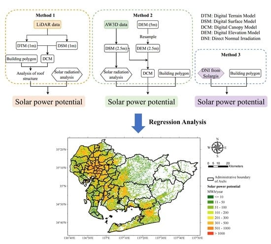
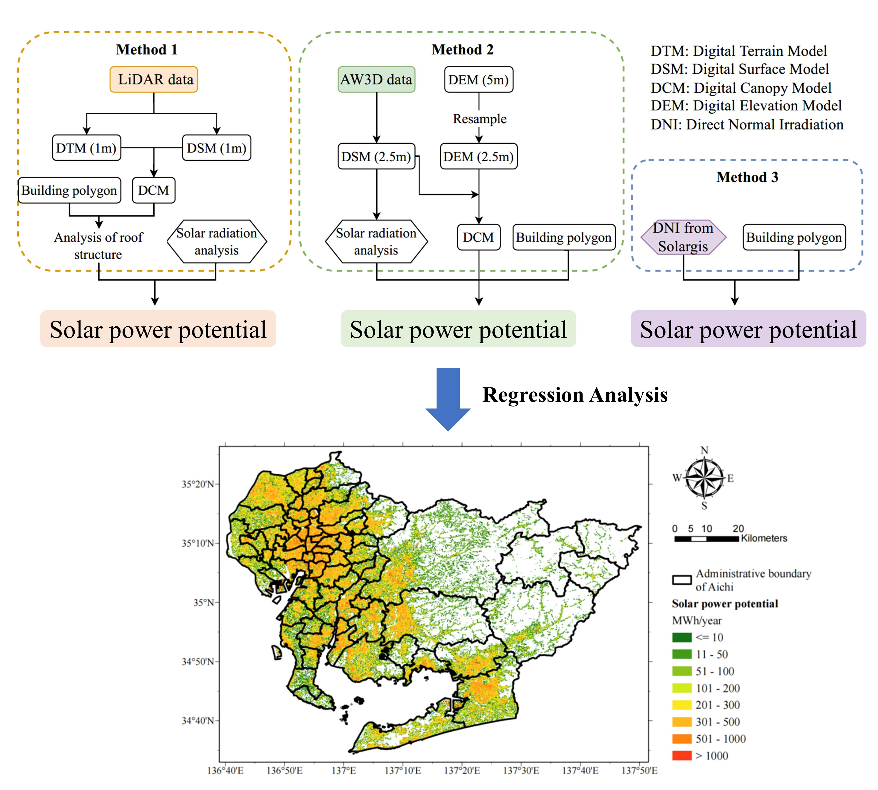
2.1. Structural Framework of the Research

In this study, we utilized three different methods to estimate the annual solar power generated by each roof (Figure 1). For each method, the results were calculated under three scenarios (maximum, medium, and minimum potential) at the current technical level. Method 1 was based on the study conducted by Matsumoto et al. [20]. First, the original LiDAR data were converted to LAS data; subsequently, a DSM was created after eliminating errors. The digital canopy model (DCM) was created by subtracting the digital terrain model (DTM) from DSM. The DCM was then combined with the building polygon data to compute the building height data, and the slope and azimuth of rooftops were estimated during the analysis of the building’s roof structure. Next, the solar radiation amount was calculated using the DSM through solar radiation analysis, considering shadow effects. Finally, the introduction potential (kW) and annual power generation amount (kWh/year) of the rooftop PV for each building were estimated.
For Method 2, the data from the AW3D Standard were utilized to create the DSM and obtain the DCM by subtracting the DEM. The remaining processes were similar to those of Method 1, without considering the slope and azimuth of rooftops. For Method 3, the introduction potential was calculated solely using the building polygon and was then combined with the direct normal irradiation (DNI) (kWh/m2/day) provided by Solargis to estimate the annual solar power generation by each roof. For all three methods, buildings with rooftop areas smaller than 10 m2 were excluded from the estimation, as described by Schunder et al. [7] and Gagnon et al. [17]. For Method 1 and Method 2, buildings with heights less than 1.5 m, as determined by the DCM, were ruled out. In addition, because buildings along the study area boundary might have their sunlight blocked by buildings outside the area, a −100 m buffer was created for the study area. Building polygons that were completely within the −100 m buffer were utilized in this study.
After obtaining the estimated annual power generation amount for each rooftop using the three methods, regression analysis was conducted to determine the relationship among the results obtained using the three methods. Finally, the annual solar power generation amount in Aichi Prefecture was estimated by combining all building polygons in Aichi and DNI from Solargis and then extrapolated to the results estimated by Method 1 through the coefficient.
ArcGIS Pro 2.7.2 (ESRI Japan) was used for the spatial analysis, Microsoft® Excel® for Microsoft 365 MSO (Version 2112) was used for the calculation, and IBM SPSS Statistics (28.0.0.0) was used for the regression analysis in this study.

2.2. Estimation of Solar Power Generation Potential in Western Aichi by Different Methods
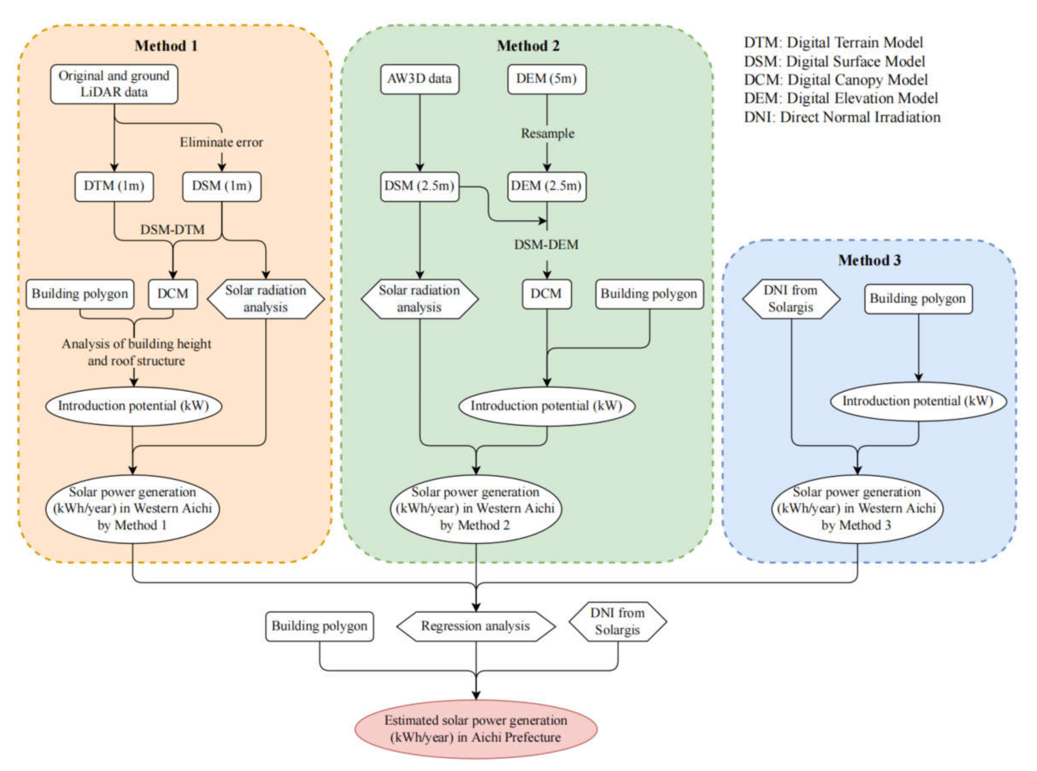
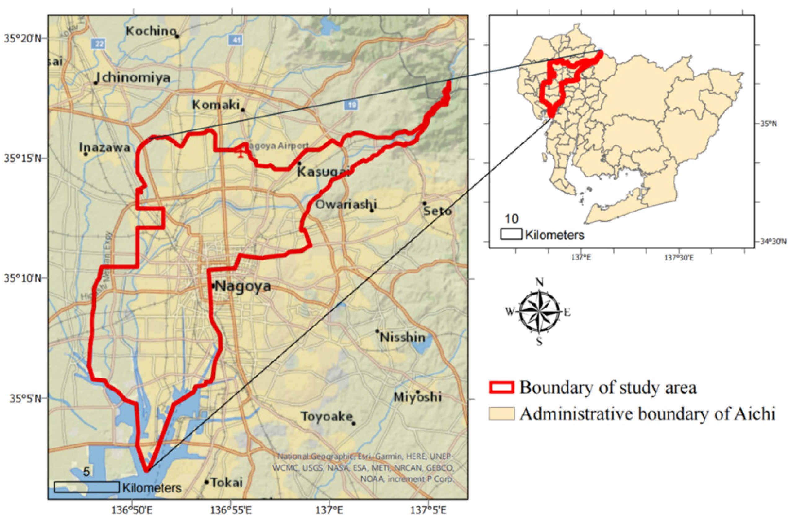
2.2.1. Study Area

The target area is the western part of Aichi Prefecture in Japan, covering 229.43 km2, as shown in Figure 2. The total number of building polygons in this area is 490,203, and the number of building polygons completely within the −100 m buffer that were included in this study was 475,764. This study used the same LiDAR data as that used in Matsumoto et al.’s study [20], but the study area, including the suburban area of Nagoya City, was expanded to approximately 1.5 times that of the previous study (152.51 km2). Aichi Prefecture (34°34′ N–35°25′ N, 136°40′ E–137°50′ E) is in the central part of Japan with a population of 7.5 million and a total area of 5173 km2 [36]. The climate of Aichi Prefecture is influenced by the Pacific Ocean’s warm current; thus, it is hot and rainy in summer and dry in winter.

2.2.2. Data Sources

An overview of the data source was shown in Table 1. For LiDAR data, the original and ground data from Shonai River and Tokigawa River Aviation Laser Survey Service (2016) provided by Geospatial Information Authority of Japan (GSI) (https://www.gsi.go.jp/ (accessed on 17 February 2022)) were used, which were the latest LiDAR data that we could obtain from the government for our study area. The AW3D data (2.5 m grid) from satellite JAXA-ALOS were purchased from JAXA, RESTEC, and NTT DATA (https://www.aw3d.jp/en/products/ (accessed on 17 February 2022)). The DNI data (250 m grid) from Solargis were downloaded from https://globalsolaratlas.info/download (accessed on 17 February 2022). The building polygon data and DEM data were obtained from GSI (https://fgd.gsi.go.jp/download/menu.php (accessed on 17 February 2022)). We used building polygon data surveyed between 2015 and 2016 to minimize the time lag with LiDAR data.

2.2.3. Method 1: Estimation of Solar Power Potential Using LiDAR Data

To estimate the maximum rooftop solar power generation potential using LiDAR data, we adopted the scheme developed by Matsumoto et al. [20], as summarized below.

2.2.3.1. Data Preparation

The average point density of the original and ground 3D point cloud LiDAR data was 13.1 points/m2 [20], which was sufficient for the analysis of aspect and angle of roof slope [37]. The original and ground LiDAR data were first converted to an LAS format file and then arranged into a 2D grid structure after classification. The classification of original LiDAR data was first conducted using the “Classify LAS Noise” tool in ArcGIS Pro, and then wire guard, power line, transmission tower, and temporary error points such as birds, smoke, and cranes were classified manually.
The “LAS Dataset to Raster” tool was used to convert original LiDAR data to DSM to analyze building height and roof structure after removing low noise, wire guard, power line, transmission tower, and high noise as classified in the original LiDAR data. The ground LiDAR data were converted to a DTM. The cell size of DSM and DTM was 1.0 × 1.0 m. The DCM, which represents the height of buildings and trees above ground level, was calculated by subtracting the DTM from the DSM, and negative values were set to 0.
The DCM was extracted by building polygon data with a buffer of −50 cm to create raster data representing the height of each building (Figure 3). The buffer was created for the building polygon data owing to the misalignment of the building polygon data and LiDAR data [20]. This reduces the error wherein the building height data are wrongly assigned to the adjacent building when the buildings are located very close to each other. After the buffer was created, 1953 building polygons disappeared because the width of the building was less than 1 m. A buffer of −50 cm was set by empirical judgment [20].

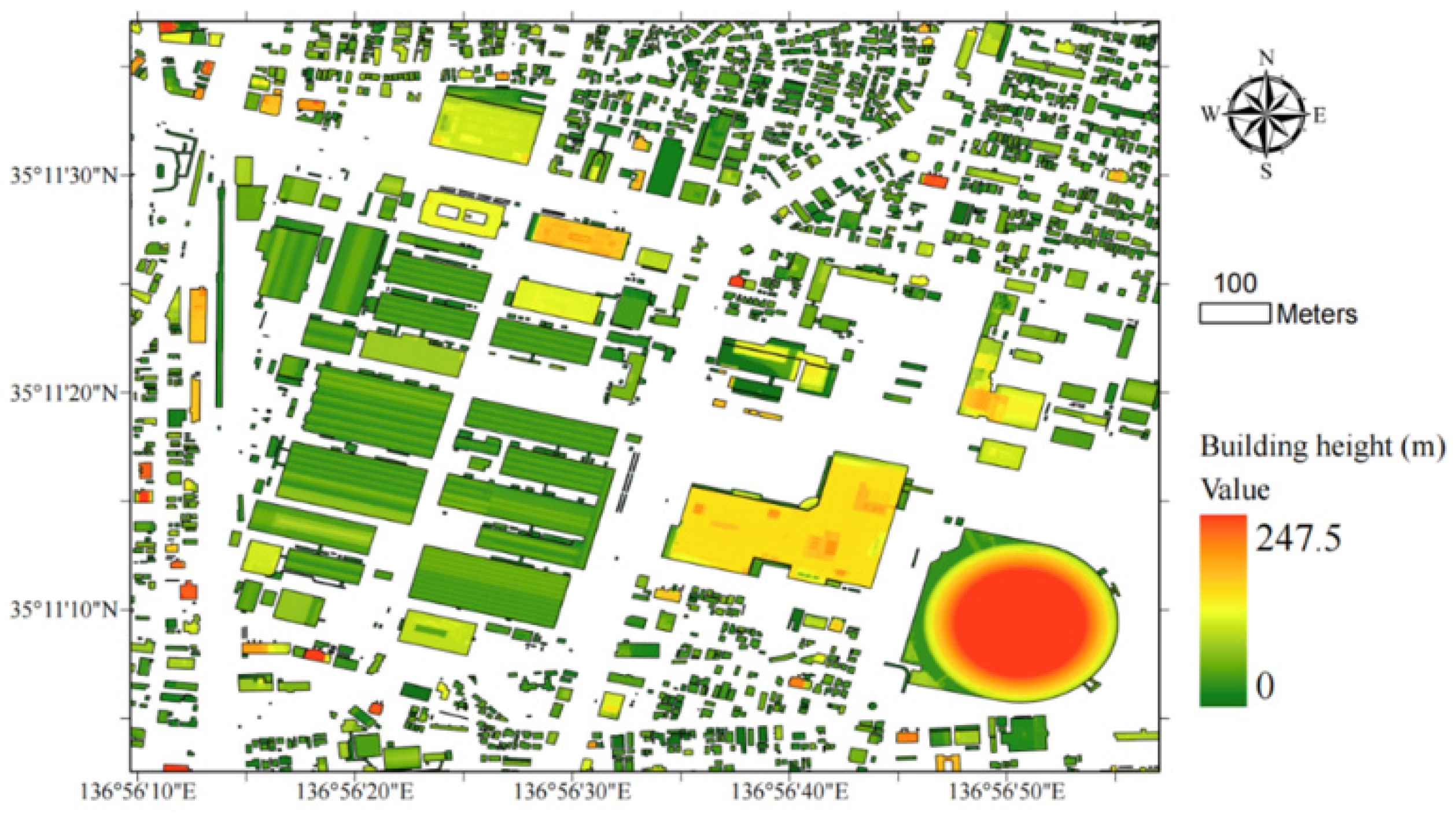
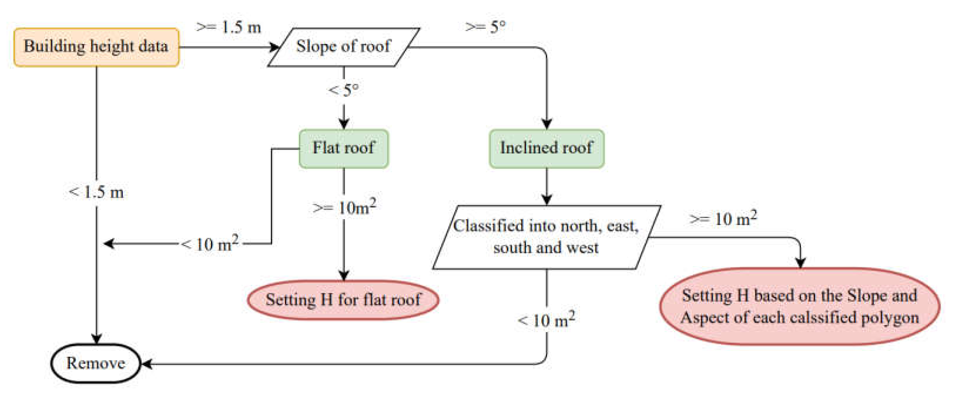
2.2.3.2. Analysis of Building Height and Roof Structure

The azimuth and slope of the roof were identified by the “Aspect” and “Slope” tools in ArcGIS Pro based on the DCM obtained in Section 2.2.3.1. The roof azimuth was expressed in 0–360° clockwise with north as 0°, and the output value was represented by −1 as the flat roof. The roof slope was expressed in 0–90°.
Building height and roof structure analyses was performed following the processes shown in Figure 4 to determine the annual average slope solar radiation “H” for flat roofs and inclined roofs, as discussed in a later section. Since the LiDAR data used in this study were surveyed in 2016, and the building polygon data were surveyed between 2015 and 2016, there is a possibility that some buildings were demolished or reconstructed during the time difference in the LiDAR data and building polygon data. Therefore, the building polygon with a height of less than 1.5 m, which was different from the 0.5 m in Matsumoto et al. [20], was removed from the study, considering the actual height of ceilings in Japan. Flat roofs were extracted using the slope data. The raster value of the slope data was rounded to the integer and approximated in 10-degree increments, and the most frequent value of the slope was calculated for each building polygon. If the most frequent value was smaller than 5°, it was assumed to be a flat roof [20]. Subsequently, the remaining inclined roofs were divided into four directions (north, east, south, and west) based on the azimuth of the rooftop. The area of each direction that was smaller than 10 m2 was excluded from the estimation, which was different from the 2 m2 cut-off area used by Matsumoto et al. [20], considering the actual floor area. The annual average slope solar radiation “H” per day of the installation surface was set based on the most common slope and aspect values in each direction.

2.2.3.3. Solar Radiation Analysis

The raster for solar radiation analysis was created using the LAS dataset described in Section 2.2.3.1 after removing low noise, power lines, and high noise. The output cell size was 1.0 × 1.0 m.
The “Area Solar Radiation” tool was used to calculate the global solar radiation of a specific area, which is the sum of direct solar and scattered solar radiations. In this study, the default values (0.3 and 0.5 of scatter rate and transmittance, respectively) were used to calculate the global solar radiation for a normal sunny day. The sky size was set to 100 m, and the daily time interval was set to 2 h, considering the capacity and time of processing. All parameters used were the same as those used by Matsumoto et al. [20]. The daily solar radiation for four particular days—the summer solstice, spring equinox, autumn equinox, and winter solstice—was calculated. By revealing the shadow from surrounding buildings, this exercise enabled the calculation of the global solar radiation (Wh/m2) for a sunny day.
The shadow factor S (Equations (1) and (2) from [20]) was used as the solar radiation amount in this study, which is the ratio of the average value of solar radiation of the four special days in each roof direction to the maximum average solar radiation amount in the target area.
S o l a v e = ( S o l s u m m e r + S o l s p r i n g , a u t u m n × 2 + S o l w i n t e r ) / 4
S = S o l a v e / S o l a v e , m a x
  • Solave: Average global solar radiation of four special days (Wh/m2).
  • Solsummer: Global solar radiation of the summer solstice (Wh/m2).
  • Solspring,autumn: Global solar radiation of the spring and autumn equinoxes (Wh/m2).
  • Solwinter: Global solar radiation of the winter solstice (Wh/m2).
  • S: Shadow factor
  • Solave,max is the maximum value of Solave in the target area (Wh/m2).

2.2.3.4. Introduction Potential

In this study, the roof surface integrated type was assumed for solar panel installation because of its excellent appearance and conversion efficiency. In addition, panels can be installed on up to 96% of the roof area [38], which can maximize the use of the roof area, similar to Matsumoto et al. [20]. The introduction potential of each roof can be estimated using the following equation [20,39]:
P = I × A × α
  • P: Introduction potential (installation capacity) (kW).
  • I: Conversion efficiency of the solar panel (kW/m2).
  • A: Rooftop area (m2).
  • α : Installable area rate of the solar panel.
In terms of A, if the roof was inclined, the sum of the areas of the four directions was used. The area of the building polygon was used for the flat roof. The value of A was corrected by the original size of the building polygon before the creation of the −50 cm buffer. By applying Equation (3), the introduction potential was estimated for each roof of each building in the target area.

2.2.3.5. Estimated Annual Solar Power Generation Amount

The estimated annual solar power generation amount was calculated using the following equation, referring to NEDO [40] and Matsumoto et al. [20]:
E p = H × S × K × P × 365 ÷ 1
  • Ep: Annual solar power generation amount (kWh/year).
  • H: Annual average slope solar radiation per day (kWh/m2/day).
  • S: Shadow factor.
  • K: Loss factor.
  • P: Introduction potential (installation capacity) (kW).
  • “365”: Number of days in a year (day).
  • “1”: Solar radiation intensity under standard conditions (kWh/m2).
The “Solar Radiation Database” from MONSOLA-11 provided by NEDO [41] was used for the value of “H” (Table 2).
The loss factor K is a variable coefficient, as it varies depending on the type of equipment installed, and it can be calculated by the following equation referring to NEDO [40]:
K = 1 L c × 1 L p × 1 L d
  • 𝐿c: Loss due to cell temperature rise.
  • 𝐿p: Loss due to power conditioner.
  • 𝐿d: Other loss such as dirt on light-receiving surface.
Therefore, by applying Equation (4), the annual power generation for each roof was estimated.

2.2.4. Method 2: Estimation of Solar Power Potential Using AW3D Data

Method 2 was similar to Method 1 but it did not analyze the roof structure. The 2.5 m grid DSM was created from the AW3D Standard, which is a high-resolution digital 3D map based on PRISM data acquired by the Advanced Land Observing Satellite (ALOS) from JAXA. Solar radiation analysis was conducted using the DSM following the processes described in Section 2.2.3.3. The 5 m grid DEM was obtained from the website of the Fundamental Geospatial Information Download Service provided by the Geospatial Information Authority of Japan (https://fgd.gsi.go.jp/download/menu.php (accessed on 8 February 2022)). The elevation void-fill function was used to create pixels where holes existed in the DEM data. The DEM was resampled to 2.5 m (the same resolution as that of DSM), and the DCM was calculated by subtracting the DEM from the DSM using the “Raster Calculator” tool, and negative values were set to 0.
The DCM was extracted using the building polygon data and then converted to an integer. The Zonal Statistics as Table function in ArcGIS Pro was performed to obtain the majority value of the DCM for each building polygon, which represented the building height. A building with a height less than 1.5 m or a rooftop area smaller than 10 m2 was excluded from the estimation, as in the LiDAR analysis.
The introduction potential of each roof is calculated using Equation (3). The annual solar power generation amount was estimated using Equation (4), and H = 3.74 was used, assuming that all the roofs were flat.

2.2.5. Method 3: Estimation of Solar Power Potential Using Solargis Data

In this method, the globally available DNI raster data (250 m grid) prepared by Solargis and published by the World Bank Group was utilized (downloaded from https://globalsolaratlas.info/download (accessed on 1 February 2022)). For this method, the introduction potential was calculated solely from the building polygon data using Equation (3), and any building polygon with an area smaller than 10 m2 was not considered in the estimation.
The DNI raster data were extracted from the study area, and the largest value was 3.686 kWh/m2/day. The raster data were converted to points, and the spatial join function was applied to attach the DNI value to the closest building polygon so that each building polygon had a DNI value. The shadow factor S was calculated as the DNI value attached to each building polygon divided by the maximum DNI value in the study area, which was 3.686 kWh/m2/day. The annual solar power generation amount for each building was estimated using Equation (4), and H = 3.74 was used, assuming that all the roofs were flat.

2.2.6. Three Scenarios Based on Variable Coefficients

Three scenarios were set based on the variable coefficients of I, α, and K, which were updated from Matsumoto et al. [20] using the recent manufacturer’s information (Table 3). The coefficient I stands for the conversion efficiency of the PV module, and the value ranges from 0.142 to 0.226 among 88 solar PV products from 11 panel manufacturers in the Japanese market [42,43,44,45,46,47,48,49,50,51,52]. The α represents the percentage of rooftop area which can be installed with solar PV, and the maximum value 96% was found in Kaname Solar [38]. The minimum value of α, 32.4%, was the average ratio of the solar panel installation area to the roof area calculated from the solar panel detection data in Nagoya City as described by Matsumoto et al. [20]. The K is the overall loss factor multiplied by the 𝐿c (Loss due to cell temperature rise), 𝐿p (Loss due to power conditioner) and 𝐿d (Other loss, such as dirt). The values for 𝐿c (0.046–0.150) and 𝐿p (0.03–0.06) varied between manufacturers of solar PVs and power conditioners, and since there was no large difference for 𝐿d between manufacturers, the constant value 0.05 was used [42,43,44,45,46,47,48,49,50,51,52].
Scenario A was used to obtain the maximum potential at the current technology level, using the upper limit of the three variable coefficients I, α, and K. Scenario B was used to obtain the standard potential at the current technology level using the average value of I and K and the median of α. Scenario C was used to find the least available potential at the current technology level using the minimum value of I, α, and K.

2.2.7. Regression Analysis

Regression analysis was carried out for the annual solar power amount generated by each building’s roof to determine the relationship between the results estimated by Method 3 and Method 1 and between Method 1 and Method 2. The building polygons were included in the simple linear regression analysis only when the results estimated by all three methods were larger than 0. The number of building polygons used in the regression analysis was 283,501. In addition, regression analysis was performed for flat and inclined roofs.

2.3. Estimated Solar Power Generation Potential in Aichi Prefecture

The solar power generation potential in Aichi Prefecture was estimated by Method 3 and extrapolated to the results estimated by Method 1, which is the most accurate method. The building polygon data of the year 2020–2021 was downloaded from the GSI (https://fgd.gsi.go.jp/download/mapGis.php (accessed on 19 February 2022)). Building polygons with areas smaller than 10 m2 were excluded. After the solar power generation potential for each building was calculated by Method 3, the result was multiplied by the ratio of the total electricity generation potential of solar PV in the study area estimated by Method 1 to the total electricity generation potential of solar PV in the study area estimated by Method 3, representing the hypothetical result estimated by Method 1. The results under scenario B were integrated into a 125 m grid using the “Summarize Within” function to create a heatmap of solar power potential for Aichi Prefecture.

3. Results

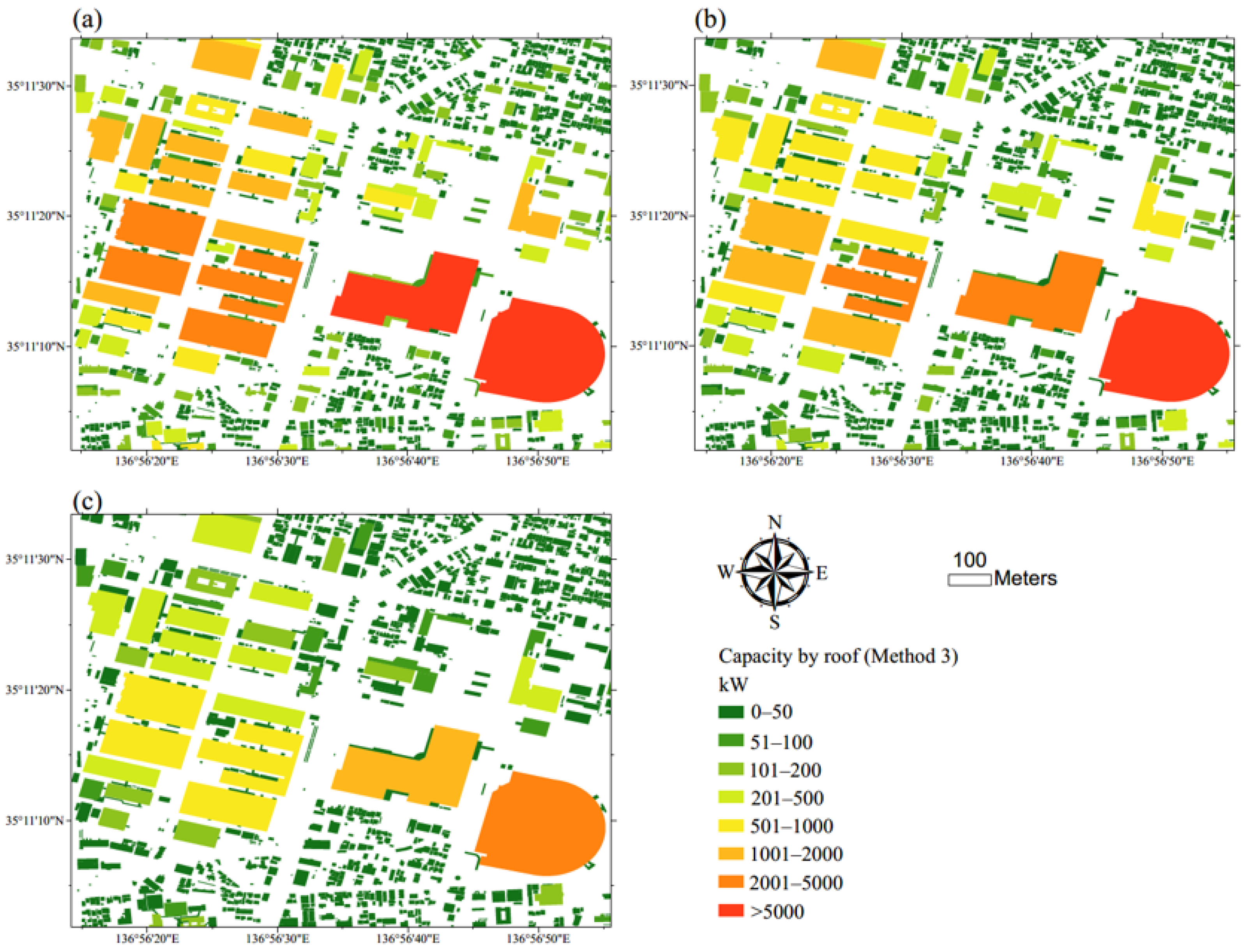
3.1. Estimation of Introduction Potential of Each Roof

The introduction potential (installed capacity) of the solar PV of each roof in western Aichi was calculated using three methods under scenarios A, B, and C. The total introduction potential of solar PV in western Aichi and the total number of buildings with introduction potential estimated by the three methods are listed in Table 4. The total number of buildings with an introduction potential of solar PV estimated by Method 3 was the largest, followed by Method 1 and Method 2. For Method 3, because the introduction potential was solely estimated from the building polygon data without building height data, buildings with an area less than 10 m2 were excluded. For Methods 1 and 2, in addition to buildings with an area less than 10 m2, buildings with a height less than 1.5 m determined by the DCM were also excluded. Because the building height was determined by DCM created from LiDAR data and AW3D data in Method 1 and Method 2, respectively, the number of buildings with heights lower than 1.5 m in Method 2 (126,823) was much larger than that in Method 1 (46,059). Therefore, the total number of buildings with an introduction potential of solar PV in Method 2 was smaller than that in Method 1.
An example of the introduction potential of each roof estimated by Method 3 under three scenarios in a part of the study area is shown in Figure 5. The maximum potential at the current technology level is depicted in scenario A, the standard potential is shown in scenario B, and the least available potential appears in scenario C. Because the value of the introduction potential of each roof was only determined by the rooftop area, the potential increased with the area.

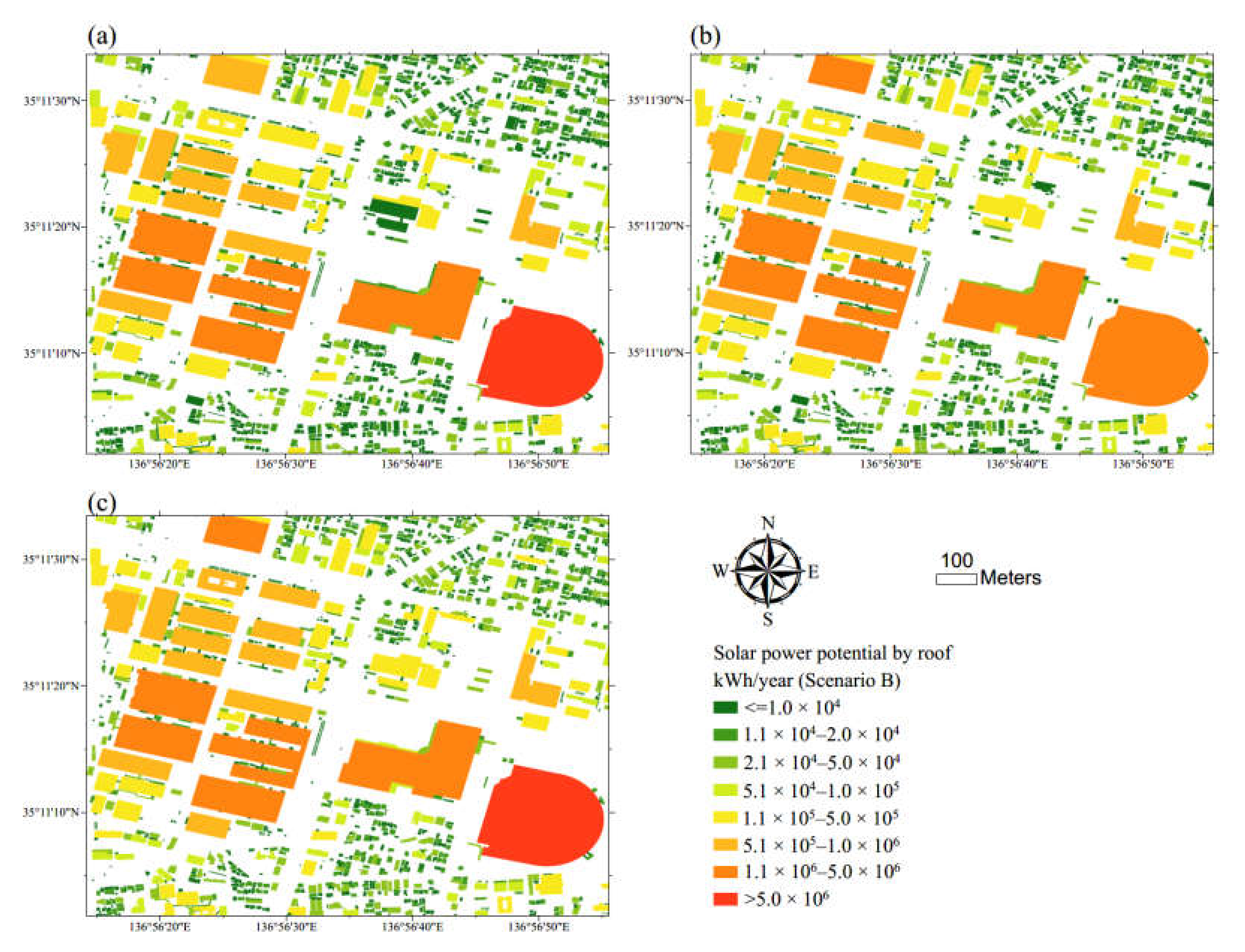
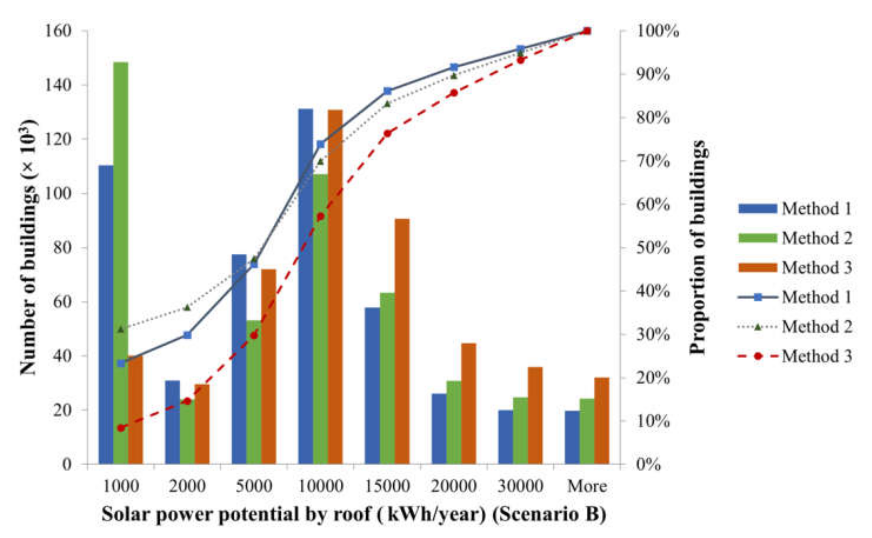
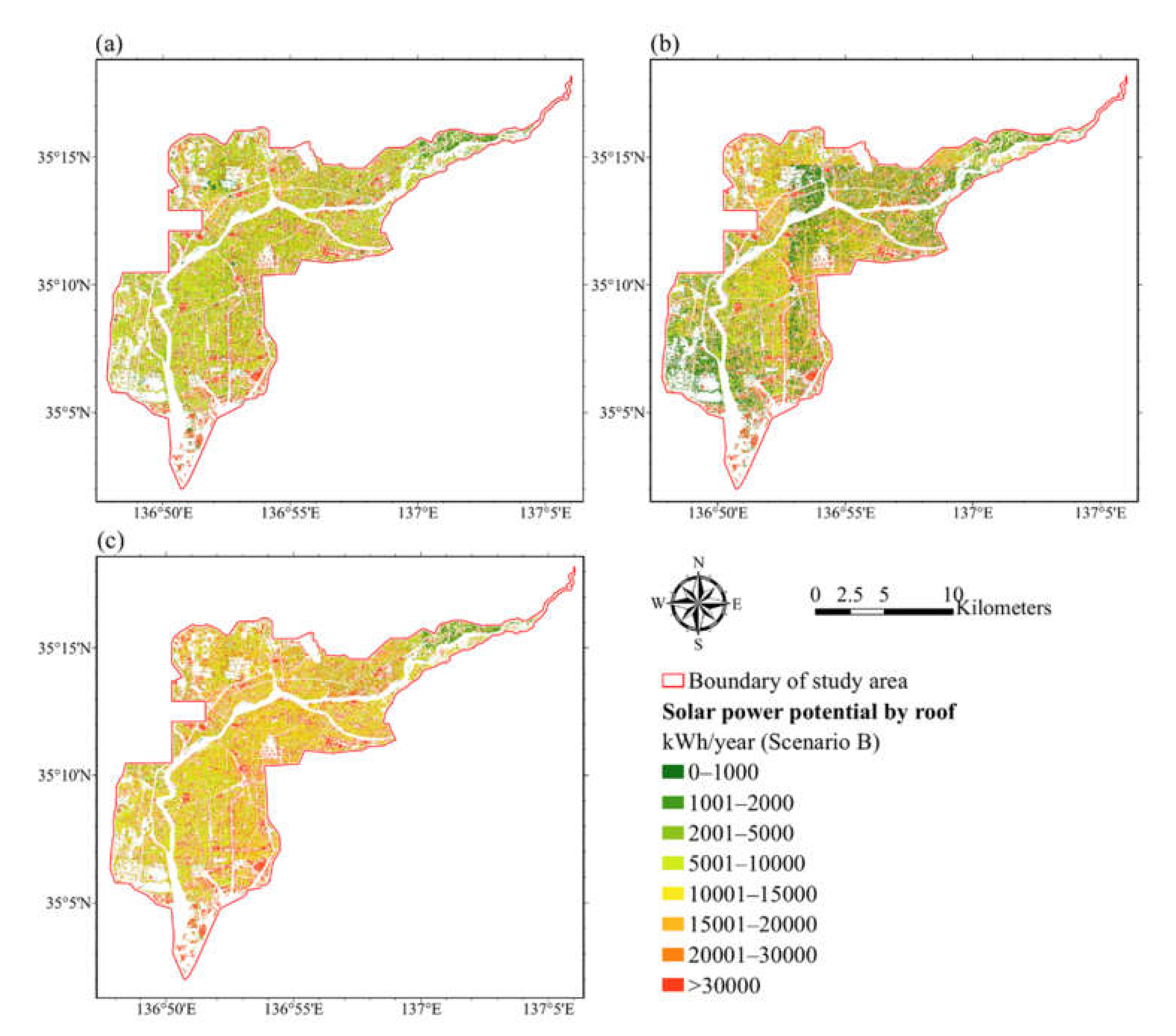
3.2. Estimation of Annual Solar Power Generation in Western Aichi by Different Methods

The annual power generation by solar PV of each roof in western Aichi was estimated using three methods under scenarios A, B, and C. Table 5 shows the total electricity generation potential of solar PV in western Aichi and the total number of building polygons with an electricity generation potential as estimated by the three methods. The total electricity generation potential of solar PV in the study area estimated by Method 1 was approximately 70% of the result calculated by Method 3, and the result estimated by Method 2 was approximately 75% of the result of Method 3. The number of buildings with an electricity generation potential of solar PV estimated by Method 3 (435,676) was the largest, followed by Method 1 (371,755) and Method 2 (327,582). At this stage, due to lack of electricity generation potential, the building polygon without solar radiation data was excluded from the estimation.
Figure 6 shows an example of the electricity generation potential of solar PV by each building’s roof estimated by the three methods under Scenario B in a part of the study area. Buildings with large rooftop areas have higher solar power generation potential. Conversely, a small building beside large, tall buildings has lower solar power generation potential due to the shadow effect of the surrounding buildings.
Figure 7 shows differences in the estimation results of the solar power potential of each roof calculated through different methods under Scenario B in part of western Aichi. This figure illustrates that there is a greater difference between the results from different methods when a roof with a large area was the subject. Additionally, the solar power potential of the large roof estimated using LiDAR data (Method 1) and AW3D data (Method 2) was less than the result estimated by Solargis data (Method 3).
The number and cumulative proportion of buildings in terms of the solar power potential of each roof (kWh/year) in the study area estimated by the three methods under Scenario B are shown in Figure 8. The total number of buildings was 475,764, including buildings without solar power potential (height lower than 1.5 m or roof area less than 10 m2). The standard potential of annual solar power generation of more than 90% of buildings at the current technology level (Scenario B) was smaller than 30,000 kWh/year in the study area estimated by the three methods. For Method 2, the annual solar power potential of 31% of the total buildings was under 1000 kWh/year. This was because 126,823 buildings lacked solar power potential due to the fact that their height was less than the 1.5 m set by the DCM based on the AW3D data. Excluding this factor, the majority (22.5%, estimated by Method 2, to 27.7%, estimated by Method 1) of total buildings in the study area had an annual solar power potential between 5000 and 10,000 kWh/year. Method 1 included the analysis of roof structure, while Method 2 and Method 3 treated all roofs as flat, and parameter H for a flat roof (3.74) was larger than most of the other angles and aspects in Table 2; therefore, the distribution of the number of buildings shifted left for Method 1 in Figure 8. In terms of buildings with solar power potential larger than 10,000 kWh/year under Scenario B, the number of buildings in Methods 2 and 3 was higher than that in Method 1, because the buildings with large roof areas included some factories whose roofs were not flat. In this case, the solar power potential estimated by Methods 2 and 3 would be greater than that estimated by Method 1.
The electricity generation potential of solar PV estimated by the three methods in western Aichi under Scenario B is shown in Figure 9. The distribution pattern of solar power generation potential was similar for all the three methods. As for Method 2, since 26.7% of the total buildings in the study area were excluded due to the building height, the excluded buildings were mostly located in the southwestern and northern regions of the study area, which is the rural part of Nagoya City.

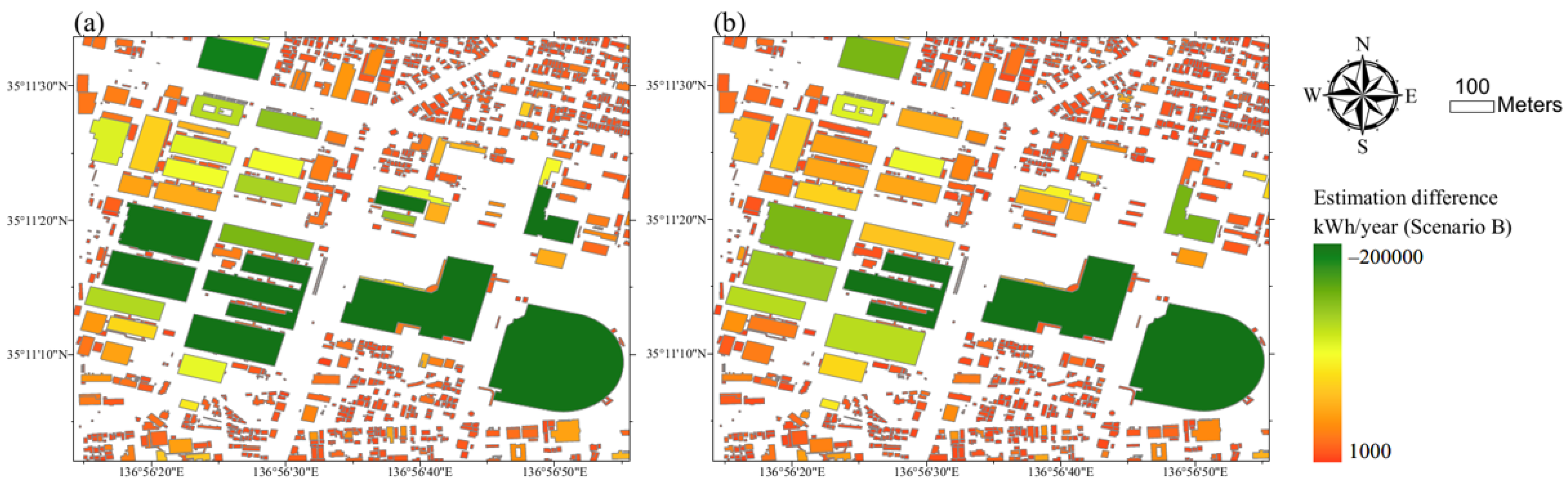
3.3. Regression Analysis

Regression analysis was performed between the annual solar power generation potential for each roof calculated by Method 3 and Method 1, as well as between Method 3 and Method 2 under scenario B.
In addition, regression analysis was conducted for flat roofs and inclined roofs, which were classified during the analysis of the roof structure in Method 1. The parameters of the regression analysis are listed in Table 6. The value of R-square was notably high, indicating a strong relationship between the results calculated by different methods.

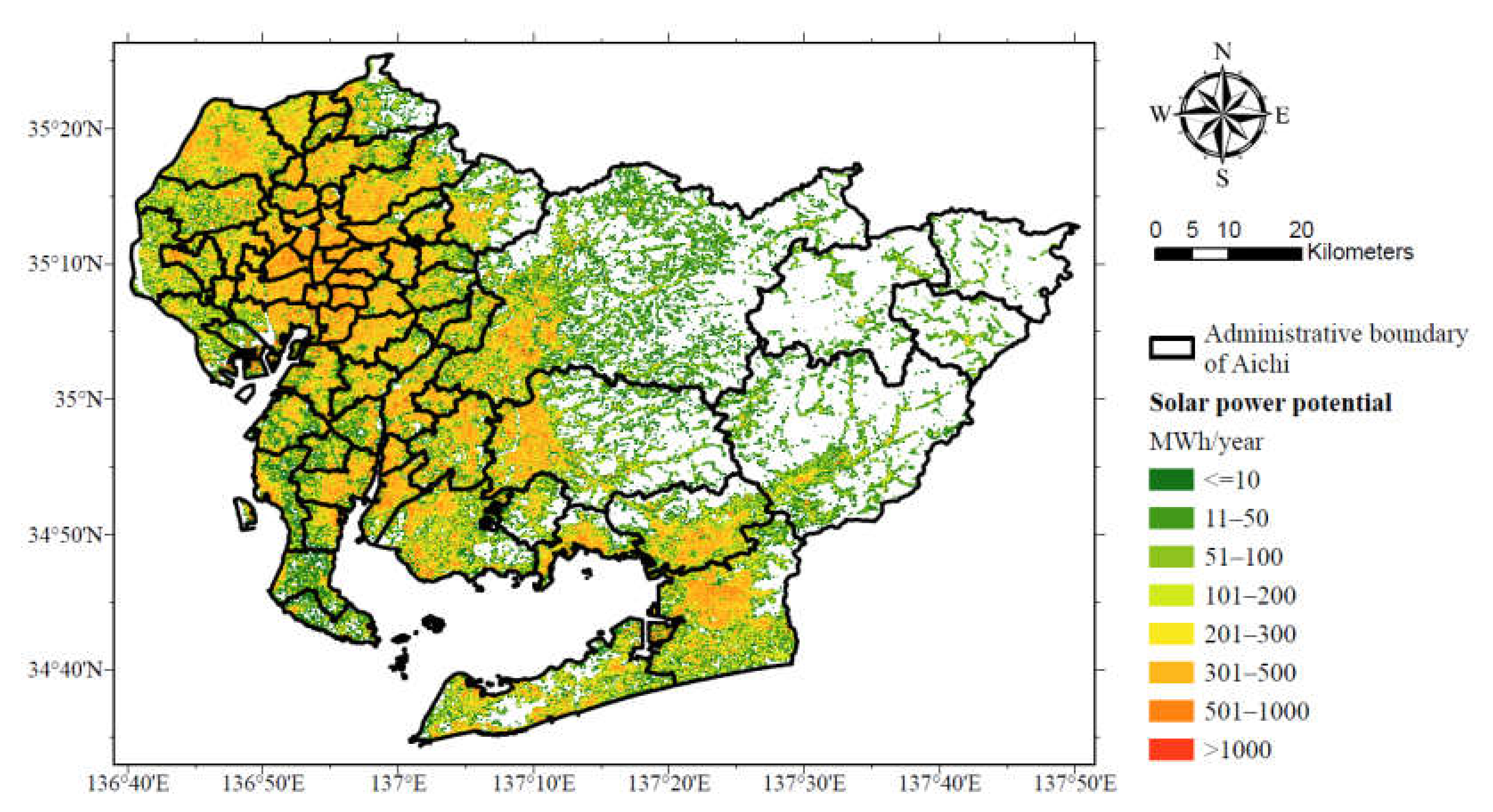
3.4. Rooftop Solar Power Potential in Aichi Prefecture

The estimated annual rooftop solar power generation amount in Aichi Prefecture was 3.58 × 10⁷ MWh/year under Scenario B (Figure 10), 6.92 × 10⁷ MWh/year under Scenario A, and 1.27 × 10⁷ MWh/year under Scenario C. The total number of building polygons included in the calculation was 3,351,960 (excluding buildings with roof areas smaller than 10 m2). The total residential electricity consumption in Aichi was 5.15 × 10⁷ MWh in 2019 [53], indicating that the rooftop solar power could satisfy the residential power demand if all the available roofs were installed with solar panels under Scenario A. The rooftop solar PV potential was mainly concentrated in the western region of Aichi Prefecture, especially in Nagoya City, because it is an urbanized city with numerous high-rise buildings. The solar PV potential in the eastern part was low because the area was mountainous and sparsely populated.

4. Discussion

4.1. Parameter Settings

For Method 1 in this study, we referred to the methodology of Matsumoto et al. [20]. However, we made revisions to the parameters regarding the variable coefficients used for the calculation in three scenarios, the threshold of the minimum height of the building and the minimum rooftop area (Table 7).
In terms of the variable coefficients I, α, and K, our approach varied from that of Matsumoto et al. [20] in that we considered two other panel brands and checked the updated parameters for 88 solar panels and 87 power conditioners in total. For the α used in Scenario C, we used the average ratio of the solar panel installation area to the roof area calculated from the solar panel detection data in Nagoya City from Matsumoto et al. [20]. For the threshold of the minimum rooftop area, we adopted 10 m2, referring to Schunder et al. [7] and Gagnon et al. [17], in contrast to the 2 m2 used by Matsumoto et al. [20]. In addition, we checked the rooftop area of 22,832 buildings detected with solar panel installation using the data from Matsumoto et al. [20] and found that 99.9% of buildings had rooftop areas larger than 10 m2 and the remaining 0.1% were smaller due to misalignment of panels and building polygons or errors in polygons.
According to the Enforcement Regulation of Building Standard Law, 2020, the height of a living room ceiling should be at least 2.1 m in Japan [54]. However, in Aichi, if 2.5 m were used as the lower limit of building height for the estimation of solar power potential, 235,220 buildings, constituting almost 48% of buildings in the study area, would be excluded based on the DCM created by the AW3D data. This could be attributed to the time lag between the AW3D Standard, acquired by the JAXA-ALOS satellite, and the building polygons provided by the GSI. Moreover, the effects of smoothed sheer edges in buildings could be another causative factor [55]. Therefore, we used 1.5 m as the lower building height limit for the estimation.

4.2. Comparison of the Three Methods

Comparing the three methods applied in this study, Method 1 using the LiDAR data was the most sophisticated and precise, and Method 3 using the Solargis data was the simplest and most convenient. Method 1 utilized high-resolution LiDAR data to create building height data and conduct a solar radiation analysis. It also included the analysis of the roof structure in determining the azimuth and slope of the roof to estimate the annual electricity generation amount by solar PV in each roof direction because the annual average slope solar radiation H was different for each combination of slope and aspect. Method 2 used 2.5 m resolution AW3D data and did not carry out the roof structure analysis, so all the roofs were treated as flat. Because H = 3.74 was used to estimate all the roofs, and it was larger than the value for the roofs facing east, west, and north (Table 2), the total annual solar power generation potential in western Aichi estimated by Method 2 was 7% higher than the results estimated by Method 1, although the total number of buildings included in the estimation was 13% less than that of Method 1. Method 3 directly utilized the DNI from Solargis as the solar radiation data instead of the solar radiation analysis using GIS. However, because the DNI from Solargis did not consider the shadow effect of the surrounding buildings and trees, the shadow factor S would be larger than the values in Method 1 and Method 2. In addition, H = 3.74 was also used for all the roofs in Method 3, so the results estimated by Method 3 were the largest. Although the results estimated by Method 1 had the highest accuracy, the analysis processes were considerably more complicated than in Method 3, and the high-resolution LiDAR data were difficult to obtain; therefore, Method 3 could be a feasible alternative when the data source was limited.

4.3. Regression Analysis

We conducted a regression analysis among the three methods to determine the relationship and conversion factor from Method 3 to Method 1. Because Method 3 was easy to adopt but overestimated the result, and Method 1 was sophisticated and time-consuming with high accuracy, a conversion factor could be obtained to extrapolate the result from Method 3 to a more realistic result for Method 1. Moreover, regression analysis was also performed for flat and inclined roofs because the annual average slope solar radiation H had different values for flat and inclined roofs when estimating the rooftop solar power potential using Method 1. In the case of Japan, most of the houses in rural areas are detached with inclined roofs, while high-rise buildings with flat roofs predominate in the urban region. The general equation for all roofs was y = 0.837x to convert the results of Method 3 to Method 1. In addition, y = 0.837x could be applied to the urban region, and y = 0.836x could be applied in the countryside if the study focus was on each building. If the situation is similar in other countries, this relationship can be utilized. However, when the estimation of solar power potential over a wide area is the main topic of research, a coefficient of 0.7 (the ratio of total annual solar power generation potential in the study area estimated by Method 1 to the result estimated by Method 3) could be applied to the result estimated by Method 3.

4.4. Comparison with Other Studies

Because of the high price, long processing times, and complicated procedures when using high-resolution remote sensing data, previous studies considering rooftop shape during the estimation of rooftop solar power potential usually used small study areas. Mavsar et al. [16] utilized LiDAR data to estimate the rooftop PV potential for a school center in Slovenia. LiDAR data were also used by Nelson and Grubesic [19], Tiwari et al. [56], and Quirós et al. [18] to assess rooftop PV potential, and the study areas were 0.265, 0.45, and 36 km2, respectively. The solar PV potential of a 5 km2 area in Beijing was estimated using 0.9 m resolution Pleiades DSM and 0.2 m resolution satellite images [25]. Similarly, Mansouri Kouhestani et al. [57] evaluated the technical and economic potential of rooftop solar power for 55,877 buildings in Lethbridge, Alberta, Canada using 1 m resolution LiDAR data. High-resolution remote sensing data can be applied to a precise evaluation of the rooftop solar power potential for a small area. However, it is difficult and time-consuming to apply to a large area.
Some studies also carried out the estimation of rooftop solar PV potential for a wide region. Joshi et al. [58] assessed global rooftop solar PV potential by demarcating rooftop area from the global landcover layer with 100 m resolution and assumed that 100% of the estimated rooftop area was available for solar PV installation. The potential PV capacity of China’s 239 airports was evaluated, and the available area of terminals and parking lots was measured by Google Earth Pro [59]. Hołuj et al. [60] estimated rooftop solar PV potential in three urban sprawls in Poland including the analysis of azimuth and angle of each roof; however, they used average annual sunlight for the calculation and did not consider the shadow effect. Monna et al. [32] explored the solar PV potential on the rooftops of residential buildings in Jordan, but they just selected four types of building typologies and the available roof area were determined for each type. Solar energy potential of urban buildings including roof and façade area were calculated for 10 cities in China, considering shading effects and weather impacts, but the analysis of roof structure was omitted [61]. Studies which estimated rooftop PV potential covering a large region usually only took into account rooftop area, but the roof morphology was neglected; however, the modeling of roof structure is necessary for the precise evaluation of solar power potential, since the received solar radiation on the rooftop is diverse for different azimuths.
Our study used three different approaches to estimate rooftop solar power potential for an area of 229 km2, including 475,764 buildings. For the LiDAR analysis, we modeled roof structure including slope and azimuth for each building, and the detailed assessment of solar radiation for each roof considering the shadow effect was also conducted. Moreover, through the regression analysis between different approaches, we developed a method with general applicability for vast areas with high accuracy when high-resolution remote sensing data are not available. This methodology could facilitate city planning for the penetration of solar PVs and the analysis of energy structure.

4.5. Limitations

The estimation of global solar radiation by LiDAR and AW3D data was performed using the solar radiation analysis tool in ArcGIS Pro, and the higher the spatial and temporal resolution of the analysis, the more accurate the results. However, because the processing capacity of the PC used was limited (Core i9-9900X, RTX 2080Ti, 64 GB memory), the sky size was set to 100 m and the daily time interval was set to 2 h, using the average of four particular days: the summer solstice, spring equinox, autumn equinox, and winter solstice. In future work, it will be necessary to calculate the monthly average solar radiation for each of the 12 months with a larger sky size and a shorter daily time interval and verify the accuracy.
Regarding Method 2, this study used 2.5 m raster data from the AW3D Standard that covers the entire global land area, to calculate the DCM and perform the solar radiation analysis. There is a more precise DSM in a 0.5 m grid from AW3D Enhanced, but it does not cover the whole region. If an accurate estimation of the solar power potential for a small area is required, it may be better to use the data from AW3D Enhanced.
Although a roof structure analysis to evaluate the slope and azimuth of the roofs was included in Method 1, it produced only an approximate value, and the shape and pattern of the roof could be much more complicated in reality. Therefore, the actual installable rooftop area of the solar PV system might be smaller than that of the estimated results.
Since the purpose of this study was to estimate the maximum potential of rooftop solar power over a wide area, roofs in all directions were considered, including the north-facing roofs. However, the cost of panel installation was not considered in this study. To apply the estimated results to a regional energy policy dealing with individual buildings, it would be necessary to conduct a cost analysis in the future.
This study only considered the rooftop solar power potential. However, in the future, it will be necessary to make estimations encompassing various technological advances, such as installation on vacant lots or on the walls of high-rise buildings.

5. Conclusions

The purpose of this study was to propose a method to estimate the rooftop solar power potential over a wide area by using a conversion factor obtained from LiDAR analysis. First, this study estimated the rooftop solar power potential in western Aichi, Japan using three methods. Subsequently, a regression analysis was conducted between the results of different methods to identify a conversion factor. Next, we estimated the rooftop solar power potential in the entire Aichi Prefecture using Method 3 and adjusted it by the conversion factor to improve the results.
Before this adjustment, the rooftop solar power potential in western Aichi estimated by Method 3 was the largest. The total electricity generation potential estimated by Method 1 and Method 2 was 70% and 75% of the result calculated by Method 3. Method 1 used LiDAR data to estimate the solar power potential, including the analysis of the roof structure and was the most complicated and precise method used in this study. Method 2 utilized AW3D data and was less complicated than Method 1. Method 3 only used the building polygon data and solar radiation data from Solargis to estimate the solar power potential. The Method 3 process was the simplest, and after applying the conversion factor 0.837 obtained from the regression analysis, the results were as accurate as those estimated by Method 1. The annual rooftop solar power potential of 3,351,960 buildings in Aichi Prefecture under Scenario A, B, and C was 6.92 × 10⁷, 3.58 × 10⁷, and 1.27 × 10⁷ MWh/year, estimated using Solargis data after the adjustment. The estimated solar power potential under Scenario A could satisfy the total residential power demand in Aichi, revealing the importance of rooftop solar power in alleviating the energy crisis from urban sprawl.
In this study, a simple but holistic methodology was developed to estimate the rooftop solar power generation potential over a wide region. This method can be easily applied worldwide using globally available data from Solargis if building polygon data are available. However, the new conversion factor has to be preceded before applying this method in an area where roof structures are largely different from those in Japan, and the regression analysis between the method using solar radiation data from Solargis and the method including detailed rooftop modeling is necessary.
The results of this study would help city planners to achieve a carbon-neutral society. In future studies, the cost of panel installation should be analyzed, and the various scenarios to install the solar PV in addition to the rooftop case should also be considered.

Author Contributions

X.H. carried out data analysis and prepared the manuscript. K.H. conceptualized and supervised the research. L.T. validated the results. T.M. and Y.H. provided part of the data. Y.T. contributed with funding acquisition. All authors have read and agreed to the published version of the manuscript.

Funding

This work was conducted under the joint research program of the Institute of Materials and Systems for Sustainability (IMaSS), Nagoya University, and Chubu Electric Power Co., Inc.

Data Availability Statement

The LiDAR data used in this study were obtained from GSI for scientific research with a contract. The AW3D data were purchased from JAXA, RESTEC, and NTT DATA. DEM and building polygon data: GSI, https://fgd.gsi.go.jp/download/menu.php (accessed on 20 August 2021); solar radiation data: Solargis, https://globalsolaratlas.info/download (accessed on 17 November 2021).

Acknowledgments

This work was carried out by the joint research program of the Institute of Materials and Systems for Sustainability (IMaSS), Nagoya University, and Chubu Electric Power Co., Inc. We would like to thank the Geospatial Information Authority of Japan (GSI) for providing the data.

Conflicts of Interest

The authors declare no conflict of interest.

References

  1. Intergovernmental Panel on Climate Change [IPCC]. Summary for Policymakers. In Global Warming of 1.5 °C; Mas-son-Delmotte, V.P., Zhai, H.-O., Pörtner, D., Roberts, J., Skea, P.R., Shukla, A., Pirani, W., Moufouma-Okia, C., Péan, R., Pidcock, S., et al., Eds.; World Meteorological Organization: Geneva, Switzerland, 2018; p. 32. [Google Scholar]
  2. REN21. Renewables 2021 Global Status Report. Available online: https://www.ren21.net/wp-content/uploads/2019/05/GSR2021_Full_Report.pdf (accessed on 10 August 2021).
  3. International Energy Agency [IEA]. Global Energy Review 2020. 2020. Available online: https://www.iea.org/reports/global-energy-review-2020/renewables (accessed on 17 February 2022).
  4. Gassar, A.A.A.; Cha, S.H. Review of Geographic Information Systems-Based Rooftop Solar Photovoltaic Potential Estimation Approaches at Urban Scales. Appl. Energy 2021, 291, 116817. [Google Scholar] [CrossRef]
  5. The United Nations Environment Program [UN]; International Energy Agency [IEA]. Global Status Report for Buildings and Construction. Available online: https://wedocs.unep.org/bitstream/handle/20.500.11822/34572/GSR_ES.pdf?sequence=3&isAllowed=y (accessed on 10 August 2021).
  6. Phap, V.M.; Thu Huong, N.T.; Hanh, P.T.; Van Duy, P.; Van Binh, D. Assessment of Rooftop Solar Power Technical Potential in Hanoi City, Vietnam. J. Build. Eng. 2020, 32, 101528. [Google Scholar] [CrossRef]
  7. Schunder, T.; Yin, D.; Bagchi-Sen, S.; Rajan, K. A Spatial Analysis of the Development Potential of Rooftop and Community Solar Energy. Remote Sens. Appl. Soc. Environ. 2020, 19, 100355. [Google Scholar] [CrossRef]
  8. The Ministry of Economy, Trade and Industry [METI]. Green Growth Strategy through Achieving Carbon Neutrality in 2050 Formulated. Available online: https://www.meti.go.jp/english/press/2021/0618_002.html (accessed on 15 August 2021).
  9. Komiyama, R.; Fujii, Y. Optimal Integration Assessment of Solar PV in Japan’s Electric Power Grid. Renew. Energy 2019, 139, 1012–1028. [Google Scholar] [CrossRef]
  10. Wen, D.; Gao, W.; Qian, F.; Gu, Q.; Ren, J. Development of Solar Photovoltaic Industry and Market in China, Germany, Japan and the United States of America Using Incentive Policies. Energy Explor. Exploit. 2020, 39, 1429–1456. [Google Scholar] [CrossRef]
  11. Institute for Sustainable Energy Policies [ISEP]. Share of Electricity Generated from Renewable Energy in 2020 (Preliminary Report). Available online: https://www.isep.or.jp/en/1075/ (accessed on 1 August 2021).
  12. Shan, J.; Toth, C.K. (Eds.) Topographic Laser Ranging and Scanning: Principles and Processing; CRC Press: Boca Raton, FL, USA, 2018. [Google Scholar]
  13. Lukač, N.; Žlaus, D.; Seme, S.; Žalik, B.; Štumberger, G. Rating of Roofs’ Surfaces Regarding Their Solar Potential and Suitability for PV Systems, Based on LiDAR Data. Appl. Energy 2013, 102, 803–812. [Google Scholar] [CrossRef]
  14. Avtar, R.; Sahu, N.; Aggarwal, A.K.; Chakraborty, S.; Kharrazi, A.; Yunus, A.P.; Dou, J.; Kurniawan, T.A. Exploring Renewable Energy Resources Using Remote Sensing and GIS—A Review. Resources 2019, 8, 149. [Google Scholar] [CrossRef] [Green Version]
  15. Brito, M.C.; Redweik, P.; Catita, C.; Freitas, S.; Santos, M. 3D Solar Potential in the Urban Environment: A Case Study in Lisbon. Energies 2019, 12, 3457. [Google Scholar] [CrossRef] [Green Version]
  16. Mavsar, P.; Sredenšek, K.; Štumberger, B.; Hadžiselimović, M.; Seme, S. Simplified Method for Analyzing the Availability of Rooftop Photovoltaic Potential. Energies 2019, 12, 4233. [Google Scholar] [CrossRef] [Green Version]
  17. Gagnon, P.; Margolis, R.; Melius, J.; Phillips, C.; Elmore, R. Estimating Rooftop Solar Technical Potential across the US Using a Combination of GIS-Based Methods, Lidar Data, and Statistical Modeling. Environ. Res. Lett. 2018, 13, 024027. [Google Scholar] [CrossRef]
  18. Quirós, E.; Pozo, M.; Ceballos, J. Solar Potential of Rooftops in Cáceres City, Spain. J. Maps 2018, 14, 44–51. [Google Scholar] [CrossRef]
  19. Nelson, J.R.; Grubesic, T.H. The Use of LiDAR versus Unmanned Aerial Systems (UAS) to Assess Rooftop Solar Energy Potential. Sustain. Cities Soc. 2020, 61, 102353. [Google Scholar] [CrossRef]
  20. Matsumoto, T.; Hayashi, K.; Huang, Y.; Tomino, Y.; Nakamura, M. Study on the estimation of solar power potential of each individual roof using airborne LiDAR data—Case study in the western part of Nagoya city. J. Hum. Environ. Symbiosis 2021, 37, 141–152. [Google Scholar] [CrossRef]
  21. Tadono, T.; Takaku, J.; Tsutsui, K.; Oda, F.; Nagai, H. Status of ALOS World 3D (AW3D); Global DSM Generation. In 2015 IEEE International Geoscience and Remote Sensing Symposium (IGARSS); IEEE: Milan, Italy, 2015; pp. 3822–3825. [Google Scholar] [CrossRef]
  22. AW3D. Products. Available online: https://www.aw3d.jp/en/products/ (accessed on 1 August 2021).
  23. Omar, R.C.; Wahab, W.A.; Putri, R.F.; Roslan, R.; Baharuddin, I.N.Z. Solar Suitability Map for Office Buildings Using Integration of Remote Sensing and Geographical Information System (GIS). IOP Conf. Ser. Earth Environ. Sci. 2020, 451, 012032. [Google Scholar] [CrossRef]
  24. Principe, J.; Takeuchi, W. Supply and Demand Assessment of Solar PV as Off-Grid Option in Asia Pacific Region with Remotely Sensed Data. Remote Sens. 2019, 11, 2255. [Google Scholar] [CrossRef] [Green Version]
  25. Song, X.; Huang, Y.; Zhao, C.; Liu, Y.; Lu, Y.; Chang, Y.; Yang, J. An Approach for Estimating Solar Photovoltaic Potential Based on Rooftop Retrieval from Remote Sensing Images. Energies 2018, 11, 3172. [Google Scholar] [CrossRef] [Green Version]
  26. Fakhraian, E.; Alier, M.; Valls Dalmau, F.; Nameni, A.; Casañ Guerrero, M.J. The Urban Rooftop Photovoltaic Potential Determination. Sustainability 2021, 13, 7447. [Google Scholar] [CrossRef]
  27. Stack, V.; Narine, L.L. Sustainability at Auburn University: Assessing Rooftop Solar Energy Potential for Electricity Generation with Remote Sensing and GIS in a Southern US Campus. Sustainability 2022, 14, 626. [Google Scholar] [CrossRef]
  28. Sánchez-Aparicio, M.; Del Pozo, S.; Martín-Jiménez, J.A.; González-González, E.; Andrés-Anaya, P.; Lagüela, S. Influence of LiDAR Point Cloud Density in the Geometric Characterization of Rooftops for Solar Photovoltaic Studies in Cities. Remote Sens. 2020, 12, 3726. [Google Scholar] [CrossRef]
  29. Al-Quraan, A.; Al-Mahmodi, M.; Al-Asemi, T.; Bafleh, A.; Bdour, M.; Muhsen, H.; Malkawi, A. A New Configuration of Roof Photovoltaic System for Limited Area Applications—A Case Study in KSA. Buildings 2022, 12, 92. [Google Scholar] [CrossRef]
  30. Ghaleb, B.; Asif, M. Assessment of Solar PV Potential in Commercial Buildings. Renew. Energy 2022, 187, 618–630. [Google Scholar] [CrossRef]
  31. Wang, Y.; Li, S.; Teng, F.; Lin, Y.; Wang, M.; Cai, H. Improved Mask R-CNN for Rural Building Roof Type Recognition from UAV High-Resolution Images: A Case Study in Hunan Province, China. Remote Sens. 2022, 14, 265. [Google Scholar] [CrossRef]
  32. Monna, S.; Abdallah, R.; Juaidi, A.; Albatayneh, A.; Zapata-Sierra, A.J.; Manzano-Agugliaro, F. Potential Electricity Production by Installing Photovoltaic Systems on the Rooftops of Residential Buildings in Jordan: An Approach to Climate Change Mitigation. Energies 2022, 15, 496. [Google Scholar] [CrossRef]
  33. Khan, M.; Asif, M.; Stach, E. Rooftop PV Potential in the Residential Sector of the Kingdom of Saudi Arabia. Buildings 2017, 7, 46. [Google Scholar] [CrossRef]
  34. Schallenberg-Rodríguez, J. Photovoltaic Techno-Economical Potential on Roofs in Regions and Islands: The Case of the Canary Islands. Methodological Review and Methodology Proposal. Renew. Sustain. Energy Rev. 2013, 20, 219–239. [Google Scholar] [CrossRef]
  35. Pavlović, T.; Milosavljević, D.; Radonjić, I.; Pantić, L.; Radivojević, A.; Pavlović, M. Possibility of Electricity Generation Using PV Solar Plants in Serbia. Renew. Sustain. Energy Rev. 2013, 20, 201–218. [Google Scholar] [CrossRef]
  36. Aichi Prefectural Government. Statistical Data of Aichi. Available online: https://www.pref.aichi.jp/global/en/ (accessed on 10 August 2021).
  37. Kodysh, J.B.; Omitaomu, O.A.; Bhaduri, B.L.; Neish, B.S. Methodology for estimating solar potential on multiple building rooftops for photovoltaic systems. Sustain. Cities Soc. 2013, 8, 31–41. [Google Scholar] [CrossRef]
  38. Kaname Solar. Kaname Solar Roof. Available online: http://www.caname-solar.jp/product/solar_roof/faq.html (accessed on 15 November 2021).
  39. Ministry of the Environment, Japan. Study on Basic Zoning Information Concerning Renewable Energies (FY2013); Ministry of the Environment: Tokyo, Japan, 2013; pp. 16–45.
  40. New Energy and Industrial Technology Development Organization [NEDO]. Solar Power Introduction Guidebook; NEDO: Tokyo, Japan, 2000; p. 76. [Google Scholar]
  41. New Energy and Industrial Technology Development Organization [NEDO]. Solar Radiation Database. Available online: https://www.nedo.go.jp/library/nissharyou.html (accessed on 20 July 2021).
  42. Canadian Solar. Solar Power Module Product Information. Available online: https://csisolar.co.jp/tax_products/module/ (accessed on 12 December 2021).
  43. Choshu Industry. Solar Power Generation System. Available online: https://cic-solar.jp/products/solar-system/#g_series (accessed on 12 December 2021).
  44. DMM.makesolar. Solar Power Generation System for Residential Use. Available online: https://energy.dmm.com/en/solar (accessed on 12 December 2021).
  45. Kyocera. Solar Power Generation and Storage Batteries: Product Information. Available online: https://www.kyocera.co.jp/solar/products/ (accessed on 12 December 2021).
  46. Next Energy. Photovoltaic Modules: Residential Products. Available online: https://pd.nextenergy.jp/solar_cell_module/residential.html (accessed on 12 December 2021).
  47. Panasonic. Panasonic Solar Power Generation System: Product Information. Available online: https://sumai.panasonic.jp/solar/lineup.html (accessed on 12 December 2021).
  48. Q Cells. Q Cells Solar Modules. Available online: https://www.q-cells.jp/products/residential_info (accessed on 12 December 2021).
  49. Sharp. Solar Power Generation System for Residential Use. Available online: https://jp.sharp/catalog/pdf/energy-sunvista.pdf (accessed on 12 December 2021).
  50. Solar Frontier. Photovoltaic Module Product List. Available online: https://www.solar-frontier.com/jpn/residential/products/modules/index.html (accessed on 12 December 2021).
  51. Toshiba. Solar Power Generation System for Residential Use. Available online: http://www.toshiba.co.jp/pv/h-solar/powerful/system/index_j.htm (accessed on 12 December 2021).
  52. XSOL. Photovoltaic Module Product Lineup. Available online: https://www.xsol.co.jp/product/lineup/module_log/ (accessed on 12 December 2021).
  53. METI, Japan. Energy Consumption Statistics by Prefecture. Available online: https://www.enecho.meti.go.jp/statistics/energy_consumption/ec002/results.html#headline2 (accessed on 1 August 2021).
  54. e-Gov Japan. Enforcement Regulation of Building Standard Law. Article 21. Available online: https://elaws.e-gov.go.jp/document?lawid=325CO0000000338 (accessed on 15 December 2021).
  55. Takaku, J.; Tadono, T.; Tsutsui, K.; Ichikawa, M. Validation of aw3d global dsm generated from alos prism. ISPRS Ann. Photogramm. Remote Sens. Spat. Inf. Sci. 2016, III–4, 25–31. [Google Scholar] [CrossRef] [Green Version]
  56. Tiwari, A.; Meir, I.A.; Karnieli, A. Object-Based Image Procedures for Assessing the Solar Energy Photovoltaic Potential of Heterogeneous Rooftops Using Airborne LiDAR and Orthophoto. Remote Sens. 2020, 12, 223. [Google Scholar] [CrossRef] [Green Version]
  57. Mansouri Kouhestani, F.; Byrne, J.; Johnson, D.; Spencer, L.; Hazendonk, P.; Brown, B. Evaluating Solar Energy Technical and Economic Potential on Rooftops in an Urban Setting: The City of Lethbridge, Canada. Int. J. Energy Environ. Eng. 2019, 10, 13–32. [Google Scholar] [CrossRef] [Green Version]
  58. Joshi, S.; Mittal, S.; Holloway, P.; Shukla, P.R.; Ó Gallachóir, B.; Glynn, J. High Resolution Global Spatiotemporal Assessment of Rooftop Solar Photovoltaics Potential for Renewable Electricity Generation. Nat. Commun. 2021, 12, 5738. [Google Scholar] [CrossRef] [PubMed]
  59. Jiang, M.; Qi, L.; Yu, Z.; Wu, D.; Si, P.; Li, P.; Wei, W.; Yu, X.; Yan, J. National Level Assessment of Using Existing Airport Infrastructures for Photovoltaic Deployment. Appl. Energy 2021, 298, 117195. [Google Scholar] [CrossRef]
  60. Hołuj, A.; Ilba, M.; Lityński, P.; Majewski, K.; Semczuk, M.; Serafin, P. Photovoltaic Solar Energy from Urban Sprawl: Potential for Poland. Energies 2021, 14, 8576. [Google Scholar] [CrossRef]
  61. Cheng, L.; Zhang, F.; Li, S.; Mao, J.; Xu, H.; Ju, W.; Liu, X.; Wu, J.; Min, K.; Zhang, X.; et al. Solar Energy Potential of Urban Buildings in 10 Cities of China. Energy 2020, 196, 117038. [Google Scholar] [CrossRef]
Figure 1. Structural framework of this study.
Remotesensing 14 01742 g001
Figure 2. Geographical location of the study area.
Remotesensing 14 01742 g002
Figure 3. Building height data in a part of the target area (the value of building height is the average value in 1 m2 after LiDAR data arrangement).
Remotesensing 14 01742 g003
Figure 4. Flow of the analysis of building height and roof structure.
Remotesensing 14 01742 g004
Figure 5. Introduction potential of each roof under three scenarios in a part of western Aichi using Solargis data (Method 3): (a) Scenario A, (b) Scenario B, and (c) Scenario C.
Remotesensing 14 01742 g005
Figure 6. The electricity generation potential of solar photovoltaic (PV) estimated by three methods in a part of western Aichi (Scenario B): (a) Method 1 (b) Method 2 (c) Method 3.
Remotesensing 14 01742 g006
Figure 7. The differences in the estimation of solar power potential of each roof (a) between Method 1 and Method 3 (b) between Method 2 and Method 3 under Scenario B (kWh/year).
Remotesensing 14 01742 g007
Figure 8. Number and cumulative proportion of buildings in relation to the solar power potential of each roof (kWh/year) in study area estimated by three methods under Scenario B.
Remotesensing 14 01742 g008
Figure 9. The electricity generation potential of solar photovoltaic (PV) estimated by three methods in western Aichi (Scenario B): (a) Method 1 (b) Method 2 (c) Method 3.
Remotesensing 14 01742 g009
Figure 10. Estimated annual rooftop solar power generation amount in Aichi Prefecture under Scenario B (the results were summarized into a 125 m grid).
Remotesensing 14 01742 g010
Table 1. Overview of the data source.
DataSpatial ResolutionTimeData Source
Original and ground data of LiDAR Surveyed in 2016 and published in 2017GSI
AW3D2.5 m × 2.5 mPublished in 2019JAXA, RESTEC and NTT DATA
DEM5 m × 5 m2020GSI
DNI250 m × 250 m2020Solargis
Building polygon shapefile 2015–2016GSI
Table 2. Annual average slope solar radiation per day for Nagoya City (kWh/m2/day).
Aspect (°)
South (0°)1530456075East, West (90°)105120135150165North (180°)
Slope (°)03.743.743.743.743.743.743.743.743.743.743.743.743.74
103.983.973.943.903.843.773.703.633.553.493.443.413.40
204.134.124.073.993.883.763.623.483.343.213.113.043.01
304.214.184.124.013.863.693.503.293.092.902.742.632.59
404.184.164.083.943.783.573.343.092.842.602.392.262.22
504.074.043.953.813.623.403.152.872.592.312.081.941.90
603.863.833.753.613.423.192.932.652.352.061.811.671.63
703.573.553.473.343.162.952.692.412.121.851.611.451.40
803.213.203.133.022.872.672.442.181.911.661.441.291.24
902.802.792.752.672.552.382.181.951.721.491.311.191.14
Source: NEDO Solar Radiation Database [41].
Table 3. Three scenarios of variable coefficients I, α, and K.
ScenarioABC
DescriptionMaximum Potential at Current Technology LevelStandard Potential at Current Technology LevelMinimum Potential at Current Technology Level
I0.2260.1920.142
α0.9600.6420.324
K0.8790.8000.759
Table 4. Total introduction potential of solar PV in western Aichi by three methods under each scenario.
MethodTotal Introduction Potential in Western Aichi (kW)Number of Buildings with Introduction PotentialBuildings without Introduction Potential
Scenario AScenario BScenario C
19.75 × 1065.54 × 1062.07 × 106375,698Rooftop area < 10 m2 or building height < 1.5 m
28.95 × 1065.08 × 1061.90 × 106327,582Rooftop area < 10 m2 or building height < 1.5 m
31.08 × 1076.14 × 1062.29 × 106435,676Rooftop area < 10 m2
Table 5. Total electricity generation potential of solar PV in western Aichi estimated by three methods under each scenario.
MethodTotal Electricity Generation Potential (kWh/year)Number of Buildings with Solar Power Potential
Scenario AScenario BScenario C
18.88 × 1094.59 × 1091.63 × 109371,755
29.51 × 1094.92 × 1091.74 × 109327,582
31.27 × 10106.58 × 1092.33 × 109435,676
Table 6. Parameters of the regression analysis of solar power potential for each building estimated by different methods.
Regression AnalysisAll RoofsFlat RoofsInclined Roofs
No. of building polygons283,50163,650219,851
Method 3 (y) vs. Method 1 (x)y = 0.837xy = 0.837xy = 0.836x
R20.9920.9920.992
Standard Error460169933625
Method 3 (y) vs. Method 2 (x)y = 0.889xy = 0.885xy = 0.894x
R20.9980.9970.998
Standard Error255241091845
Table 7. Comparison of parameter settings of this study and those used by Matsumoto et al. [20].
Matsumoto et al. [20]This Study
Method 1Method 2Method 3
Data used LiDAR data and building polygonsLiDAR data and building polygonsAW3D data and building polygonsSolar radiation data and building polygons
Study areaWestern Nagoya (152.51 km2 and 298,903 buildings)Western Aichi (229.43 km2 and 490,203 buildings)
Minimum building height (m)0.51.5
Minimum rooftop area (m2)210
Variable coefficients I, α, and K Scenario AScenario BScenario C Scenario AScenario BScenario C
I0.2210.1880.147I0.2260.1920.142
α0.9600.7200.480α0.9600.6420.324
K0.8790.8020.751K0.8790.8000.759
Number of panel manufacturers checked9 (including 56 solar panel products and 46 power conditioners)11 (including 88 solar panel products and 87 power conditioners)
Publisher’s Note: MDPI stays neutral with regard to jurisdictional claims in published maps and institutional affiliations.

