Article

Data-Driven Joint Beam Selection and Power Allocation for Multiple Target Tracking

1
School of Computer Science and Technology, Zhoukou Normal University, Zhoukou 466001, China
2
National Laboratory of Radar Signal Processing, Xidian University, Xi’an 710071, China
*
Author to whom correspondence should be addressed.
Remote Sens. 2022, 14(7), 1674; https://doi.org/10.3390/rs14071674
Submission received: 8 March 2022 / Revised: 29 March 2022 / Accepted: 29 March 2022 / Published: 30 March 2022
(This article belongs to the Special Issue Radar Signal Processing for Target Tracking)

Abstract

:
For the problem of joint beam selection and power allocation (JBSPA) for multiple target tracking (MTT), existing works tend to allocate resources only considering the MTT performance at the current tracking time instant. However, in this way, it cannot guarantee the long-term MTT performance in the future. If the JBSPA not only considers the tracking performance at the current tracking time instant but also at the future tracking time instant, the allocation results are theoretically able to enhance the long-term tracking performance and the robustness of tracking. Motivated by this, the JBSPA is formulated as a model-free Markov decision process (MDP) problem, and solved with a data-driven method in this article, i.e., deep reinforcement learning (DRL). With DRL, the optimal policy is given by learning from the massive interacting data of the DRL agent and environment. In addition, in order to ensure the information prediction performance of target state in maneuvering target scenarios, a data-driven method is developed based on Long-short term memory (LSTM) incorporating the Gaussian mixture model (GMM), which is called LSTM-GMM for short. This method can realize the state prediction by learning the regularity of nonlinear state transitions of maneuvering targets, where the GMM is used to describe the target motion uncertainty in LSTM. Simulation results have shown the effectiveness of the proposed method.

1. Introduction

Multiple target tracking (MTT) is an important research topic in the military field, and also a difficult problem at present [1,2,3]. Multiple-input multiple-output (MIMO) [4] radar is an extension of traditional phased array radar, and it is able to transmit signals in all directions and multi-beams at the same time. This operating mode is called simultaneous multi-beam mode [5]. Technically speaking, in the simultaneous multi-beam mode, a single collocated MIMO radar can track multiple targets simultaneously by controlling different beams tracking different targets independently. In this case, the complex data association process of tracking can be avoided since the spatial diversity of multiple targets can be used to distinguish the echoes of different targets, and thus, the multi-target tracking problem can be divided into multiple single-target tracking problems.
In practical applications, we have to consider two limiting factors inherent to collocated MIMO radar [6]. (1) The maximum number of beams that the system can generate is limited at each time. In theory, if the number of MIMO radar transmitters is N, the system can only generate M ( M < N ) orthogonal beams at most at each time. (2) The total transmitted power of simultaneous multiple beams is limited by the hardware. In real applications, it is necessary to limit the total transmitted power of multiple beams to ensure that the total transmission power of the system does not exceed the tolerance of the hardware. With the traditional transmitting mode, the number of beams is always set to a constant, and the transmitting power is uniformly allocated to the beams. Although it is easy to implement in engineering, the utilization efficiency of the resource is relatively low. In terms of the kinds of resources, the existing resource allocation methods can be roughly divided into two groups: one is based on the transmitting parameters, the other is based on the system composition structure. In this paper, the discussed problem of power and beam resource allocation belongs to the first one. The resource allocation based on the system composition structure mostly exists in multiple radar systems (MRS).
In [7], the authors used the covariance matrix of the tracking filter as the evaluation of tracking performance, and established and solved an optimization cost function of transmitted power. The authors of [8] proposed a cognitive MTT method based on prior information, and designed a cognitive target tracking framework. With this method, the radar transmit power parameters can be adaptively adjusted at each tracking time based on the information fed back by the tracker. In [9], an MRS resource allocation method is proposed for MTT based on quality of service constrained (QoSC). This method cannot only illuminate multiple targets in groups, but also optimize the transmitted power of each radar. The authors of [10,11,12,13,14] also studied the optimization-based resource allocation method with different resources limitation in different target–radar scenarios. Their similarity is to take the localization Cramér–Rao lower bound (CRLB) or the tracking Bayesian Cramér–Rao lower bound (BCRLB) [13] as the performance evaluation in the cost function. However, the used CRLBs and BCRLBs are both derived with an assumption of constant velocity (CV) model or constant acceleration (CA) model, we thus conclude that these kinds of methods are model-based methods. These model-based methods can achieve excellent results on the premise that the target’s motion is conform to the model assumption. However, in the case of maneuvering targets (the targets undergoing non-uniform-linear motions with certain uncertainty and randomness), they would not work well because the inevitable model mismatch causes a lower resource utilization, a larger prediction error of the target state, and an unreliable BCRLB. To overcome this, in [15], the resource problem was first formulated as a Markov decision process (MDP) and solved by a data-driven method, where recurrent neural network (RNN) [16,17] was used to learn a prediction model for BCRLB and target’s state, and deep-reinforcement-learning (DRL) [18,19] was adopted for solving the optimal power allocation solution. This method works under the condition that the number of generated beams is equal to the number of targets. However, in practice, radar system always have to face the challenge that the maximum beam number is far less than the number of targets. On this basis, the authors further propose a constrained-DRL-based MRS resource allocation method for meeting the given accuracy of single target tracking [20]. It is noticed that, in [15,20], the output of RNN is characterized as a single Gaussian distribution. In this way, an accurate predictive information can be obtained as the target is maneuvering with low uncertainty. Based on above studies, in this paper, we will further discuss how to jointly schedule the power and beam resources of a radar system to enhance the overall performance of MTT in maneuvering target scenarios.
In this paper, a novel data-driven joint beam selection and power allocation (JBSPA) method is introduced. The main contributions of this paper can be summarized as follows:
(1)
A JBSPA method for MTT is developed based on deep learning, which aims to maximize the performance of MTT by adjusting power and beam allocation within the limited resources at each illumination. Through mathematical optimization modeling and analysis, the problem of JBSPA is essentially a non-convex and nonlinear problem, and the conventional optimization method is thus not suitable. To address this problem, we characterize the original optimization cost function as a model-free MDP problem by designing and introducing a series of variable parameters of MDP, including state, action and reward. For a discrete MDP, a common way is dynamic programming (DP). However, our problem is a continuous controlling problem over the action and state space, and thus, DP-based methods are not available. Since the emerging DRL is a good model-free MDP [21], it will be taken to solve MDP of JBSPA (DRL-JBSPA) in this paper.
(2)
Considering the possible existence of a model-mismatch problem in maneuvering target tracking, the long short-term memory (LSTM) [
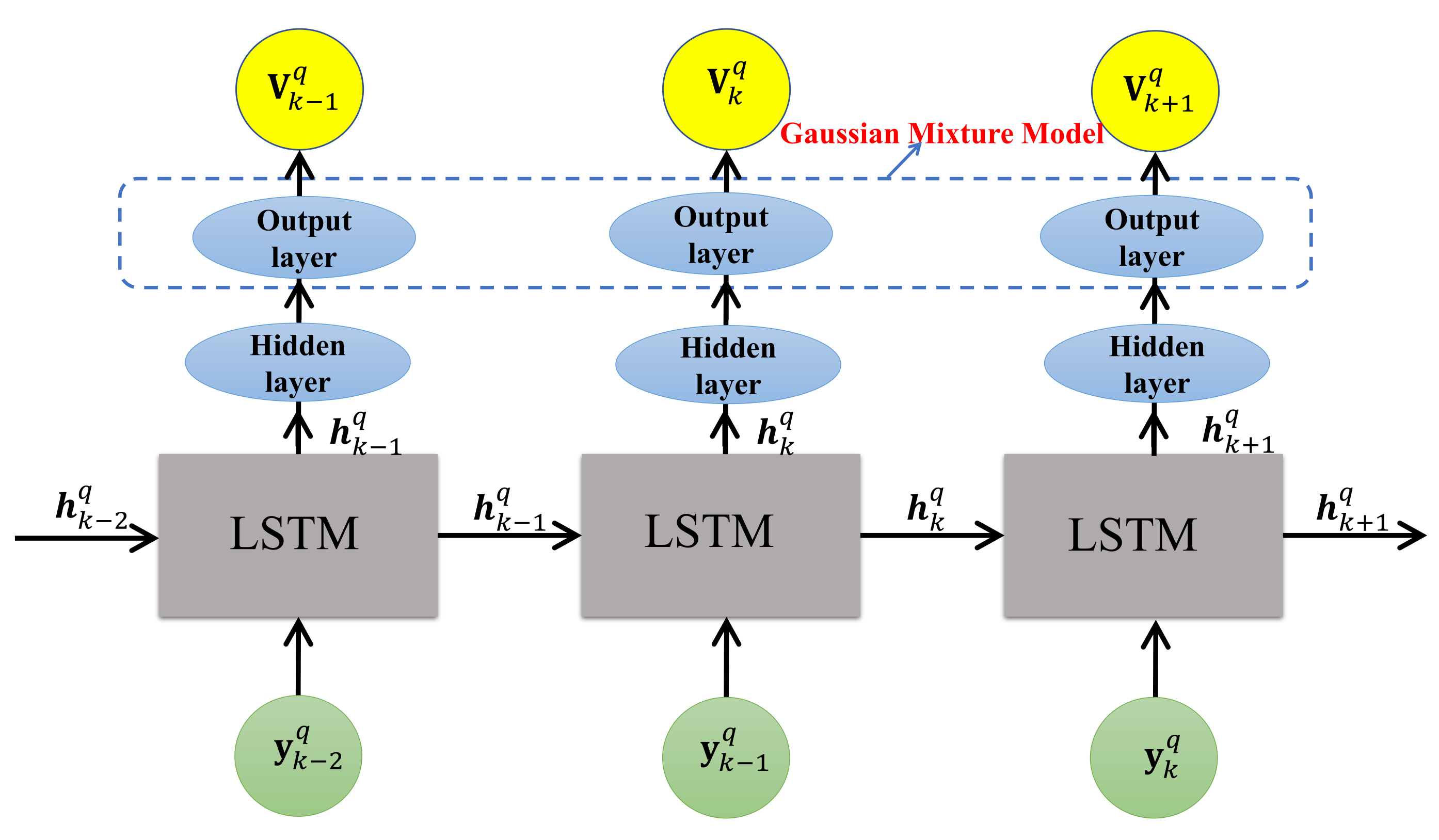
17] incorporating the Gaussian mixture model (GMM), say, LSTM-GMM, is used to derive prior information representation of targets for resource allocation. The biggest change exists in the output layer of LSTM; there, two different GMMs are utilized to describe the uncertainty of state transition of the maneuvering target and radar cross-section (RCS), respectively. In this way, at each tracking interval, the LSTM-GMM will not output a determined predicted extended target state, but multiple Gaussian distributions. Then, we select one of them randomly according to mixed coefficients, to obtain the predicted target state and RCS, and the Bayesian information matrix (BIM) of prior information at the next tracking time instant.
(3)
Considering that the JBSPA is a continuous control problem over state and action spaces, in order to improve the computational efficiency, this work adopts a deterministic policy function in calculation of Q function, and deduces the deterministic policy gradient [22,23] by deriving the Q function with respect to policy parameters. Then, we apply an actor network and a critic network to enhance the stability of the training. A modified actor network is designed to improve the applicability of the original actor-critic frame to JBSPA, where the output transmit parameters (i.e., the number of generated beams by the radar, the pointing of beams, and the power of each beam) are realized by taking three different output layers into the action network. Due to the usage of a trained network and avoiding optimization solving at each tracking time, the requirement of real time in resource allocation can be guaranteed in MTT.
The outline of the paper is as follows. In Section 2, a brief review of DRL is introduced. In Section 3, the resource allocation problem is described. In Section 3, the resource allocation problem is abstracted into a mathematical cost function. In Section 4, a deep-learning-based JBSPA method is detailed. In Section 5, several numerical experiment results are provided to verify the effectiveness of the proposed method. Some problems and future works are discussed in Section 6. In Section 7, the conclusion of this paper is given.

2. Markov Decision Process and Reinforcement Learning

In this section, a brief introduction MDP and reinforcement learning (RL) is given. Being the fundamental model, MDP is often used to describe and solve the sequential decision-making problems involving uncertainties. In general, a model-free MDP is described as a tuple S , A , r , γ , where S is the state set in the decision process, A is the action set, r is the reward feedback by the environment after executing a certain action, and γ is the discounted factor for measuring the current value of future return. The aim of MDP is to find the optimal policy that can maximize the cumulative discounted reward k = 0 γ k r t + k , and the policy function π a s is expressed as follows:
π a s = p A t = a S t = s
which is the probability of taking action a with current state s .
Due to the randomness of the policy, the expectation operation is used to calculate the cumulative discounted reward function. When an action is given under a certain state, the cumulative discounted reward function becomes the state-action value function, i.e.,
Q s , a = E π k = 0 γ k r t + k S t = s , A t = a
which is also called Q function. This function is generally used in DRL for seeking the optimal policy.
In reinforcement learning (RL), there is an agent that can interact with the environment by actions, accumulate interactive data, and learn optimal action policy. In general, the commonly used reinforcement learning methods are classed into two kinds: one is based on the value function and the other is based on the policy gradient (PG). In value-function-based RLs, such as Q-learning, the learning criteria are looking for the action that can maximize the Q function by exploring the whole action space, i.e.,
a * = arg max a Q s , a
For the applications on continuous state and action space, value-function-based methods are not always available. Different from the circuitous way of Q-learning enumerating all action-value functions, policy-gradient-based methods find the optimal policy by directly calculating the update direction of policy parameters [21]. Therefore, the PG is more suitable for MDP problems over continuous action and state space. The goal of PG is to find the policy π ϑ * that can maximize the expectation of cumulative discounted reward, i.e.,
π ϑ * = arg max π ϑ E τ ˜ π G τ ˜
where τ ˜ : S 1 , A 1 , S 2 , A 2 , S 3 , A 3 , S 4 , A 4 , represents the trajectory obtained by interacting with the environment using policy π ϑ * , and G τ ˜ denotes the cumulative discounted reward on τ ˜ . The loss function of the policy is defined as the expectation of the cumulative return, which is given by
J ϑ = E τ ˜ π G τ ˜ = τ ˜ π ϑ π ϑ τ ˜ G τ ˜ d τ ˜
where π ϑ τ ˜ represents the occurrence probability of the trajectory τ ˜ with the policy π ϑ . The policy gradient can be obtained by deriving (5), as shown in the following:
ϑ J ϑ = E τ ˜ π ϑ log π ϑ τ ˜ G τ ˜
Compared with value-function-based methods, the PG-based methods has two advantages, one is higher efficiency in the applications of continuous action and state space, the other is that randomization of the policy can be realized.

3. Problem Statement

There are a monostatic MIMO radar and Q independent point targets in the MTT scenario. The monostatic MIMO radar performs both the transmitting task and receiving task. Assume that the location of MIMO radar is x r , y r , and the targets is initially located at x 0 q , y 0 q , q = 1 , 2 , 3 , , Q . At k-th tracking time step, the q-th target’s state is given by x k q = x k q , x ˙ k q , y k q , y ˙ k q T , in which x k q , y k q and x ˙ k q , y ˙ k q denote the corresponding location and speed of q-th target, respectively. Besides that, the RCS components of targets can be also received by the radar at each time step, and that of the q-th target is denoted by ψ k q = [ h q , k R , h q , k I ] T , h q , k R and h q , k I are the RCS components of channel R and channel I, respectively. If we synthesize the target state component and the RCS component into a vector, an extended state vector can be obtained, i.e., ξ k q = x k q T , ψ k q T T .

3.1. Derivation of BCRLB Matrix on Transmitting Parameters

Before modeling JBSPA, we first deduce the mathematical relationship between the tracking BCRLB and the beam selection parameters and power parameters in this section. According to [15], with the assumption that the beam number is the same as the target number, the expression of BIM is
J m ξ k q = ξ k q 1 + E ξ k q D q , k T y k q 1 D q , k
and its inverse is BCRLB matrix, i.e.,
B C R L B x k = J m 1 x k
In (7), the term ξ k represents the covariance matrix of the predictive state error, and its inverse matrix is the Fisher information matrix (FIM) of prior information. The term E ξ k q D q , k T y k q 1 D q , k is the FIM of the data. D q , k denotes the Jacobian matrix of the measurement y k q with respect to predictive target’s state ξ k q . The term y k q 1 represents the covariance matrix of the measurement noise [24,25].
It is known that FIM of the prior information only depends on the motion model of the target, while the FIM of the data is directly proportional to the transmitted power of the radar. Assume that the transmitted power is P k = [ P 1 , k , P 2 , k , , P Q , k ] T at time step k. When P q , k is zero, that is, there is no beam allocated to the q-th target for illumination at time step k, and the covariance matrix y k q 1 of the measurement error is a zero matrix. In order to describe the beam allocation more clearly, a group of binary variables z k = [ z 1 , k , z 2 , k , , z Q , k ] T is introduced here, where
z q , k = 1 , i f P q , k > 0 0 , i f P q , k = 0
where z q , k = 1 indicates that the radar illuminates target q at the k-th tracking time instant, and z q , k = 0 is the opposite. Then, substitute (9) into (7), and we obtain [26,27]
J m ξ k q = ξ k q 1 + z q , k E ξ k q D q , k T y k q 1 D q , k
whose inverse matrix, BCRLB matrix, can be used as an evaluation function of transmitted power P q , k and beam selection parameter z q , k . The expression is as follows:
B C R L B P q , k , z q , k ξ k q = ξ k q 1 + z q , k P q , k E ξ k q D q , k T ^ y k q 1 D q , k 1
in which the original covariance matrix of the measurement error y k q 1 is rewritten as a multiplication of P q , k and ^ y k q 1 .

3.2. Problem Formulation of JBSPA

In JBSPA, since the target state ξ k q is unknown at the k 1 -th time step, a predictive state ξ k k 1 q is taken to calculate the FIM of data. In addition, in order to ensure the requirement of real-time in MTT, we use one-sampling measurement to calculate the FIM of data instead of the expectation of FIM of data. The final BCRLB matrix is given by [14]
B C R L B P q , k , z q , k ξ k k 1 q = ξ k q 1 + z q , k P q , k D ^ q , k T ^ y ^ k q 1 D ^ q , k ξ k k 1 q 1
where D ^ q , k denotes the Jacobian matrix of the measurement y ^ k q with respect to predictive target’s state ξ k k 1 q . ^ y ^ k q is the approximation of the covariance matrix of measurement at the predictive state ξ k k 1 q . In theory, the diagonal elements of the derived BCRLB matrix represent the corresponding lower bounds of the estimation MSEs of the target states, and thus, the tracking BCRLB of the target is defined as the trace of the BCRLB matrix, i.e.,
Φ P q , k , z q , k = Tr B C R L B P q , k , z q , k ξ k k 1 q
where Tr · represents trace operator. In order to enhance the MTT performance as much as possible, and ensure the tracking performance of each target, we take the worst-case tracking BCRLB among targets as an evaluation of the MTT performance to optimize the resource allocation result, which is expressed as
F P k , z k = max q Φ P q , k , z q , k
The problem of JBSPA is then described as follows: restricted by the predetermined maximum beam number M and the power budget P t o t a l , the power allocation and the beam selection are jointly optimized for the purpose of maximizing the cumulative discounted worst-case BCRLB of MTT. The cost function is written as
min P k , z k u = k K γ u k F P k , z k s . t . q = 1 Q z q , u P q , u = P t o t a l δ k = q = 1 Q z q , u M , z q , u 0 , 1 , P q , u = 0 z q , u = 0 P ¯ q min P q , u P ¯ q max z q , u = 1 u = k , , K , q = 1 , , Q
where constraints 1∼3 are the total power constraint, the beam number constraint and the single beam power constraint, respectively. P ¯ q min and P ¯ q max are the minimum and the maximum of the single beam transmitted power, respectively. Due to the existence of binary beam selection parameters, the cost function (15) is a complex mixed-integer nonlinear optimization problem. As the discount factor is γ = 0 , the cyclic minimizing method [28] and projection gradient algorithm can be used to solve the problem [14]. However, since this method needs to traverse all possible beam allocation solutions to find the optimal solution, the solving process is time-consuming. With this method, if there are a large number of targets to track, the real-time performance of MTT cannot be guaranteed. On the other hand, when the discount factor γ is non-zero, to solve the problem requires accurate future multi-step predictions of target state and BCRLB which is, however, hardly realized in real applications, especially in the scenarios involving maneuvering targets because the potential model-mismatch problem would amplify the prediction error and reduce the reliability of BCRLB seriously along with the tracking time increasing.
To address above issues, we discuss the JBSPA from MDP perspective, and solve it with a data-driven method: DRL. Compared with the optimization-based method, this method is able to avoid the multi-step prediction problem and complex solving process, and ensure the real-time performance of resource allocation. Besides that, in order to make the method suitable for maneuvering target scenarios, RNN with LSTM-GMM unit is used to learn the state transition regularity of maneuvering targets, and then realize the information prediction of the maneuvering target.

4. Joint Beam Selection and Power Allocation Strategy Based on Deep Reinforcement Learning

In this section, the original resource problem is first modeled as a model-free MDP. It is a complicated continuous controlling problem over action and state spaces. Therefore, the value-function-based DRLs, such as the DQN, are not applicable. For this problem, we choose to directly derive the Q function with respect to the policy parameters to calculate the policy gradient, and seek the optimal resource allocation policy along the descending direction of the policy gradient. In this paper, the proposed DRL-based method is named DRL–JBSPA (DRL for Joint Beam Selection and Power Allocation).

4.1. Overall

The workflow of the DRL–JBSPA system is shown in Figure 1. The implementation at each tracking interval, the current measurement of targets (i.e., radial range, angle, Doppler and RCS) will be imported into the DRL system to perform the tasks of the information prediction and the resource allocation. The prediction network has also been incorporated into the DRL system to provide the DRL agent state at each decision step. The key idea behind this design is to realize the best beam and power control by learning from the massive interaction data between the DRL agent and the environment. It is noticed that this environment here is not real, it is established artificially and consists of the agent state, action and reward. In this application, according to the objective and the resource limitations of JBSPA, the agent state, the action and the reward are designed in the following.
STATE: The state of the DRL agent is defined as
s k = ξ k k 1 1 , , ξ k k 1 q , , ξ k k 1 Q , d i a g ( ξ k 1 ) , , d i a g ( ξ k q ) , , d i a g ( ξ k Q ) T
where d i a g ( · ) represents the operation of taking the main diagonal elements. ξ k q denotes the covariance matrix of the one-step predictive state ξ k k 1 q . According to Section 3.1, the covariance matrix represents the prediction error of target state, and the agent can determine how to allocate resource by comparing the prediction error of all targets. Moreover, the predictive states of all of the targets are also included in the agent state vector, whose aim is to utilize the target state information, such as the targets’ ranges, the speeds and the RCS, to assist the agent in judgment. As γ = 0 , the DRL agent tends to allocate more power and beam resources to the targets with larger prediction errors to ensure their tracking performances [14].
ACTION: Instead of using a binary variable z k to describe the beam allocation, two action parameters δ k and X k are taken here to represent the generated beam number and determine which target to be illuminated in the next tracking time instant, respectively. δ k is a scalar and X k is
X k = X 1 , X 2 , , X Q T , X q 0 , 1 , q = 1 , 2 , , Q
Then, synthesizing the power allocation action and the two beam allocation actions into an action vector, we have
a k = δ k , X k T , P k T T
REWARD: An intuitive reward function will benefit the learning efficiency of DRL. According to the objective function in (15), we set the reward function to the opposite of the worst-case BCRLB at the k-th time step, i.e.,
r k ( s k , a k ) = l F P k , z k
where l is a constant given artificially, and used for controlling the reward scale.

4.2. LSTM-GMM Based Prediction Network

The structure of prediction network is illustrated in Figure 2, where the LSTM is used with GMM output layer, say, LSTM-GMM. At the k-th time step, this network outputs the prior information representation V k q for target q with the measurement y k 1 q as the input, which can be expressed in a mathematical form, i.e.,
V k q = f θ R y k 1 q , h k 1 q ; θ R
where f θ R ( · ) represents an abstracted function of the RNN-GMM and θ R is its parameter vector. Based on maximum likelihood, the loss function is
L θ R = ln p ξ k q
in which p ξ k q is the probability density function (PDF) of the prior distribution of the extended target state. Since the state vector and the target RCS component are independent of each other, the original PDF p ξ k q can be obtained by multiplying two independent PDFs, i.e.,
p ξ k q = p x k q p ψ k q
In this section, in order to describe the state transition of the maneuvering target and the randomness and uncertainty of the target RCS, we assume that the distributions of the target state and the target RCS are two different Gaussian mixture models that are composed of K t and K r Gaussian distributions, respectively. The PDFs are expressed as
p x k q = k t = 0 K t 1 Π q , k k t exp 1 2 x k q μ x k q k r T x k q 1 x k q μ x k q k t 2 π 2 x k q k r 1 2 , k t = 0 K t 1 Π q , k k t = 1
p ψ k q = k r = 0 K r 1 Π q , k k r exp 1 2 ψ k q μ ψ k q k r T ψ k q 1 ψ k q μ ψ k q k r 2 π 2 ψ k q k r 1 2 , k r = 0 K r 1 Π ˜ q , k k r = 1
where μ x k q k t and x k q k t are the mean and the covariance matrix of the k t -th Gaussian distribution of target state x k q , respectively. μ ψ k q k r and ψ k q k r denote the mean and the covariance matrix of the k r -th Gaussian distribution of RCS ψ k q , respectively. Π q , k k t and Π ˜ q , k k r are the corresponding mixed coefficients. Since the target state has four dimensions, the mean of the covariance matrix of K t -th mixed Gaussian distribution can be expressed as follows.
μ x k q k t = μ x q , k k t , μ x ˙ q , k k t , μ y q , k k t , μ y ˙ q , k k t T x k q k t = σ x k q k t 2 ρ 1 k t σ x k q k t σ x ˙ k q k t 0 0 ρ 1 k t σ x k q k t σ x ˙ k q k t σ x ˙ k q k t 2 0 0 0 0 σ y k q k t 2 ρ 2 k t σ y k q k t σ y ˙ k q k t 0 0 ρ 2 k t σ y k q k t σ y ˙ k q k t σ y ˙ k q k t 2
In (25), it is assumed that the target state in x-direction and y-direction are independent from each other. The terms μ x q , k k t , μ x ˙ q , k k t and σ x k q k t , σ x ˙ k q k t are the mean and the standard deviation of the K r -th Gaussian distribution of the target state on x-direction, respectively, and μ y q , k k t , μ y ˙ q , k k t and σ y k q k t , σ y ˙ k q k t denote that on y-direction. ρ 1 k t and ρ 2 k t are the correlation coefficients of the location and the speed on x-direction and y-direction, respectively. Since there are two channels of RCS, the PDF p ψ k q is a two-dimensional Gaussian, whose mean and covariance matrix are
μ ψ k q k r = μ h q , k R k r , μ h q , k I k r T ψ k q k r = σ h q , k R k r 2 0 0 σ h q , k I k r 2
where μ h q , T k R k r , μ h q , T k I k r and σ h q , T k R k r , σ h q , T k I k r represent the mean and the standard deviation of the K r Gaussian distribution on channel R and channel I, respectively.
Based on the above derivations and analysis, the output vector of RNN at the k-th time step is given in (27), and its dimension is 11 K t + 5 K r .
V k q = μ ξ k q T , σ ξ k q T , Π ξ k q T , ρ x k q T T
where
μ ξ k q = μ x q , k 1 , , μ x q , k K t , μ x ˙ q , k 1 , , μ x ˙ q , k K t , μ y q , k 1 , , μ y q , k K t , μ y ˙ q , k 1 , , μ y ˙ q , k K t , μ h q , k R 1 , , μ h q , k R K r , μ h q , k I 1 , , μ h q , k I K r T σ ξ k q = σ x q , k 1 , , σ x q , k K t , σ x ˙ q , k 1 , , σ x ˙ q , k K t , σ y q , k 1 , , σ y q , k K t , σ y ˙ q , k 1 , , σ y ˙ q , k K t , σ h q , k R 1 , , σ h q , k R K r , σ h q , k I 1 , , σ h q , k I K r T Π ξ k q = Π q , k 1 , , Π q , k K t , Π ˜ q , k 1 , , Π ˜ q , k K r T ρ x k q = ρ 1 1 , , ρ 1 K t , ρ 2 1 , . . . . , ρ 2 K t T
In the implementation, at each tracking interval, we will randomly select one from the mixed Gaussian distribution outputs as the prior distribution of the extended target state according to the mixing coefficients. Assuming the k t -th Gaussian distribution of target state and the k r -th Gaussian distribution of RCS is selected, then the predictive extended target state and the corresponding FIM of prior information J P ξ k q are given by
ξ k k 1 q = μ x q , k k t , μ x ˙ q , k k t , μ y q , k k t , μ y ˙ q , k k t , μ h q , k R k r , μ h q , k I k r T
J P ξ k q = ξ k q 1 = d i a g b l k x k q k t , ψ k q k r 1
where d i a g b l k ( · ) refers to the operation of the diagonal block matrix. Taking (29) and (30) into (13), we obtain the predicted tracking BCRLB of the q-th target at the k-th time step.
In the training stage, if the training set D = y ˜ 1 m , ξ 1 m , y ˜ 2 m , ξ 2 m , , y ˜ L ξ m , ξ L ξ m m = 1 M consists of M tracks with length L ξ , the loss of RNN is calculated by
L θ R = 1 2 m = 1 M k = 1 L ξ ξ k m μ ξ k m T ξ k m 1 ξ k m μ ξ k m
The time step of LSTM is set to L ξ and the Adam optimizer [29] is utilized with dropout. In the implementation, the probability of switching off the neuron output in the dropout function is set to 0.3.
As the prediction network structure shown in Figure 2, the structure of this network is established on a single-layer LSTM unit whose gate functions and nonlinear layer are all composed of 64 neurons. At the k-th time step, the observation vector is first normalized and then taken into the LSTM unit to execute “remember” and “forget” operations, and we obtain the final output O k after the data flow through the hidden layer and the output layer, where O k 1 4 K t + 2 K r is the extended target state component, O k 4 K t + 2 K r + 1 8 K t + 4 K r is the standard deviation of each component of the extended target state, O k 8 K t + 4 K r + 1 9 K t + 5 K r are the mixed coefficients, and O k 9 K t + 5 K r + 1 11 K t + 5 K r are the correlation coefficients.
Since the standard deviation and the mixing coefficient of each target state component are strictly non-negative, the elements O k 4 K t + 2 K r + 1 8 K t + 4 K r and O k 8 K t + 4 K r + 1 9 K t + 5 K r should be operated as follows.
O ^ k 4 K t + 2 K r + 1 8 K t + 4 K r = exp O k 4 K t + 2 K r + 1 8 K t + 4 K r
O ^ k 8 K t + 4 K r + 1 9 K t + 5 K r = exp O k 8 K t + 4 K r + 1 9 K t + 5 K r
Additionally, considering that the output O k is a standardized result, the final estimated target state is calculated using the mean and the standard deviation of the samples, i.e.,
μ ξ k q = O k 1 4 K t + 2 K r s ¯ ξ + ξ ¯ σ ξ k q = O ^ k 4 K t + 2 K r + 1 8 K t + 4 K r s ¯ ξ 2 Π ξ k q = O ^ k 8 K t + 4 K r + 1 9 K t + 5 K r O ^ k 8 K t + 4 K r + 1 9 K t + 5 K r O ^ k 8 K t + 4 K r + 1 9 K t + 5 K r O ^ k 8 K t + 4 K r + 1 9 K t + 5 K r ρ x k q = O k 9 K t + 5 K r + 1 11 K t + 5 K r
where s ¯ ξ and ξ ¯ are the mean and standard deviation of the samples, and the calculation is as follows.
ξ ¯ = 1 M L ξ m = 1 M l = 1 L x ξ l m s ¯ ξ = 1 M L ξ 1 m = 1 M l = 1 L x ξ l m ξ ¯ 2

4.3. Actor-Critic-Based DRL for JBSPA

Considering that the MDP of JBSPA is a continuous controlling problem and the traditional Q-table method is not available, we adopt the PG-based method to solve it. By introducing the policy function π ϑ a s , the original problem (5) can be characterized as a classical MDP problem, which aims to find the optimal policy parameter ϑ * that makes the Q-value function achieve the maximum, i.e.,
ϑ * = arg max ϑ Q π ϑ s k , a k
where the Q function is calculated by
Q π ϑ s k , a k = E s k + 1 ρ π , a k π ϑ a k s k r s k , a k + γ E a k + 1 π ϑ a k + 1 s k + 1 Q π ϑ s k + 1 , a k + 1
in which the symbol ρ π refers to the state space with policy π ϑ a s . According to the definition of DRL state for our problem, we know that the DRL state is determined by the current target measurement information. However, the target measurement is always random duo to the existence of observation noise. Therefore, the DRL state transition is not deterministic, i.e.,
p s k + 1 s k , a k 1
According to (37), if the random policy is used at each decision time step, a large number of samples are required to calculate the Q value of all possible actions in the continuous action space or high-dimensional discrete action space. In order to reduce the computational complexity, the deterministic policy is adopted in this section, which is expressed as
a k = μ ϑ s k
where μ ϑ ( · ) is the deterministic policy function. Then, take (39) into (37), simplify, and have
Q μ ϑ s k , a k = E s k + 1 ρ π r s k , a k + γ Q π ϑ s k + 1 , a k + 1
Next, derive the Q-value function with respect to ϑ , and obtain the following deterministic policy gradient:
ϑ J π ϑ = E s k + 1 ρ π ϑ μ ϑ s k + 1 a Q μ ϑ s k + 1 , a k + 1 a k + 1 = μ ϑ s k + 1
Subsequently, the equivalence between original problem and the established MDP problem is discussed in this section.
max ϑ Q μ ϑ s k , a k = max ϑ E s k + 1 ρ π r s k , a k + γ Q π ϑ s k + 1 , a k + 1 = min P q , k , q = 1 , , Q Φ P q , k + γ E m = k + 1 K γ m k 1 Φ P q , m = min P q , k , q = 1 , , Q E m = k + 1 K γ m k Φ P q , m
It can be seen from (42) that the MDP problem (36) is essentially the expectation form of original problem (15). In other words, the aim of the optimization problem is transformed to maximizing the expectation of the cumulative discounted MTT performance. The usage of the reinforcement learning makes it feasible to perform power allocation considering the long-term and short-term tracking performance by estimating the Q value to approximate the cumulative discounted MTT BCRLB.
Based on the derived deterministic policy gradient, this paper uses the deep deterministic policy gradient (DDPG) [22] algorithm to learn the optimal power allocation strategy based on the actor-critic framework. DDPG is a reinforcement learning algorithm that combines deep learning and the deterministic policy gradient. Its biggest advantage is that it can learn more effectively in the continuous action space. The structure of the DDPG mainly consists of two deep networks, i.e., the actor network and the critical network.
In the calculation of the Q value, the DDPG draws lessons from the idea of deep Q learning and adopts the target network with exactly the same structure as the critic-actor network to ensure the stability of network training. The DDPG prefers to update the target network parameters slightly by “soft” updating the target network, and achieve the improvement of learning stability. This operation is similar to the regular replication of parameters to the target network in the DQN. The soft update of the target network parameters is expressed as follows:
θ μ : = τ θ μ + 1 τ θ μ θ Q : = τ θ Q + 1 τ θ Q
where θ μ and θ Q are the parameters of the actor network μ · θ μ and the critic network Q · θ Q , respectively. θ μ and θ Q are the parameters of the target networks μ · θ μ and Q · θ Q , respectively. τ is the soft updating parameter which takes always a small value.
Exploration behavior is also introduced to make the DRL agent more experienced, with which the DRL agent is able to try unexplored areas to discover the improvement opportunity. At the k-th decision time step, the performed action is given by
a k = μ s k θ μ + O
where O is the random noise for agent exploration.
In order to further ensure the stability of learning, the experience relay technique is used to eliminate the strong temporal autocorrelation inherent to DRL, and can reduce the variance of the estimation of Q-values. At each training step, assuming that H experience samples are randomly selected from the experience replay buffer B to update the critic network and the actor network, the loss function of the critic network is written as
L Q θ Q = 1 H j = 1 H Q s j , a j θ Q Q j Tar 2
where Q j Tar denotes the target Q value, and is used as “labels” for the estimation of the Q-values. Q j Tar is calculated by
Q j Tar : = r j + γ Q s j , μ s j θ μ θ Q
According to (41), the policy gradient with one sampling can be obtained by
θ μ J π θ μ 1 H j = 1 H θ μ μ s θ μ s = s j a Q s , a θ Q s = s j , a = μ s j θ μ
The parameter of the actor network θ μ is synchronously updated based on the chain rule of gradient propagation. More details of the DRL–JBSPA are given in Algorithm 1.
Algorithm 1: DRL–JBSPA.
1:Randomly initialize parameters θ μ and θ Q of actor network μ · θ μ and critic network Q · θ Q ;
2:Initialize target networks θ μ θ μ , θ Q θ Q ;
3:Initialize replay buffer B;
4:for each episode do
4:   Initialize random process O for action exploration;
5:   Receive initial state s 1 derived from the prediction network
          s 1 = f θ R y 0 q , h 0 q ;
6:   for each step k of episode do
7:      Select action a k = μ s k θ μ + O ;
8:      Execute action a k and observe state s k + 1 and reward r k
             s k + 1 = f θ R y k q a k , h k q
             r k = F P k , z k ;
9:      Store transition sample s k , a k , r k , s k + 1 into replay buffer B;
10:      Sample from B a minibatch of H transitions;
11:      Calculate the target Q value:
             Q j Tar : = r j + γ Q s j , μ s j θ μ θ Q ;
12:      Update critic network by minimizing the loss:
             L Q θ Q = 1 H j = 1 H Q s j , a j θ Q Q j Tar 2 ;
13:      Update the actor network using the sampled policy gradients:
       θ μ J π θ μ 1 H j = 1 H θ μ μ s θ μ s = s j a Q s , a θ Q s = s j , a = μ s j θ μ ;
14:      Update the target networks:
             θ μ τ θ μ + 1 τ θ μ
             θ Q τ θ Q + 1 τ θ Q ;
15:   end for
16:end for
The used actor-critic network is shown in Figure 3, where the actor network contains two hidden layers and three output layers. The hidden layers are dense layers consisting of 256 neurons with ReLU activation, and the three output layers are all dense layers and share the same hidden layers. For different output actions, three output layers are named Actor 1, Actor 2 and Actor 3, respectively. Actor 1 consists of M neurons, and Actor 2 and Actor 3 are both composed of Q neurons.
At the k-th time step, the DRL state s k is first input to the hidden layer in the actor network, and then, the output of the hidden layer will be taken into Actor 1. The activation function of Actor 1 is set as the softmax function s f · , which is used to derive the probability of all possible beam numbers:
a 1 = s f w A 1 h k A + b A 1
where h k A refers to the output of the hidden layer, w A 1 and b A 1 represent the weight and the bias of Actor 1, respectively. By selecting the superscript index corresponding to the maximum probability in a 1 , the number of beams generated by the radar at the k-th time step can be determined, i.e., δ k = arg max a 1 .
Next, concatenate a 1 with the output of the hidden layer, and then send it to Actor 2. Actor 2 is responsible for determining which target will be illuminated at the next tracking time step. For this purpose, the softmax activation function is used here to output the probability of each target illuminated. The output of Actor 2 is calculated by
a 2 = s f w A 2 h k A , a 1 + b A 2
in which w A 2 and b A 2 are the weight and the bias of Actor 2. Then, the target to be illuminated can be determined by selecting the largest δ k element from a 2 , which is X k = arg max a 2 , δ k .
In the same way, we concatenate the outputs of the hidden layer, actor 1 and actor 2, and import it into actor 3. Actor 3’s activation function is set to the tanh function. The calculation formula is as follows:
a 3 = tanh w A 3 h k A , a 1 , a 2 + b A 3
where w A 3 and b A 3 are the weight and the bias of Actor 3. Select the elements in a 3 with index X k to form the vector P k , and then normalize it to obtain the ratio of each target’s allocated power to the total transmitted power. So far, by selection and splicing the outputs of the three output layers, we finally obtain the complete action vector a k = δ k , X k T , P k T T .
The critic network takes the concatenated action vector a ˜ k = a 1 , a 2 , a 3 and current agent state s k as input and outputs the corresponding Q value. The critic network consists of two dense hidden layers and an output layer, where each of the hidden layers consists of 256 neurons with ReLU activation, and the output layer is a linear neuron. In our implementation, the Adam optimizer is used to train the actor-critic network, and the learning rate is set to 1e-4. The soft updating parameter τ is set to 1e-3. The deep learning library TensorFlow is taken to implement the networks on a personal computer with Intel Core i5-7500 CPU and 16GB RAM. NVIDIA GeForce GTX 1080TI GPU is used to accelerate the training process.

5. Simulation Results

In practice, the radar system has to face the challenge that the target number is larger than the beam number. Therefore, the simulation experiments are carried out under the condition that the maximum number of beams is less than the target number. Specifically, simulation 1 is conducted to investigate the proposed method by comparing the optimization-based method with the discounted factor γ = 0 , simulation 2 is taken to discuss the effect of the discounted factor γ on the resource allocation results and the tracking performance.
The targets and the radar are depicted in the Cartesian coordinate system. Without loss of generality, the parameters of the radar system are set as follows: the radar system is assumed to be located at 0 km , 0 km , the signal effective bandwidth and effective time duration of the qth beam are set as B q , k = 2 MHz and T q , k = 1 ms, respectively. The carrier frequency of each beam is set as 1 GHz, and thus, the carrier wavelength is λ q = 0.3 m. The time interval between successive frames is set as 2 s, and a sequence of 50 frames of data are utilized to support the simulation. The lower and upper bounds of the power of the qth beam are set to P ¯ q min = 0.1 P t o t a l and P ¯ q max = P t o t a l , respectively. The maximum number of beams is 5 and the target number is 8. For better illustration of the effectiveness of the proposed method, the initial positions and initial velocities of the targets are set the same, i.e., ( 1 e 5 m , 1 e 5 m ) and ± 200 m / s , ± 200 m / s . The turning frequency of turn motion targets is set to 0.0035 Hz. The motion parameters of each target have been listed in Table 1, where the symbol “*” indicates that a motion mode does not include this motion parameter. The real moving trajectories of the three targets are depicted in Figure 4. As shown in Figure 4, Target 1 and Target 4 are doing right-turn motion, Target 2, Target 5 and Target 8 are doing left-turn motion; Target 3, Target 6 and Target 7 are doing uniform linear motion.
The prediction network is first trained for deriving prior information representation, where the training examples are the measurements of the targets’ states with the trajectories of left-turn motion, right-turn motion, and uniform linear motion, and the corresponding labels are true targets’ states. The initial position and the speed of the targets are randomly generated within [50 km, 150 km] and [−300 m/s, 300 m/s] on x-axis and y-axis, respectively. The turning frequencies are randomly generated within [0.001 Hz, 0.008 Hz]. In the process of generating training examples, the noise power added in measurements is determined by the allocated transmit power that is randomly generated within the interval P ¯ q min , P ¯ q max . We trained RNN over 200,000 epochs, and AC-JBSPA over 500,000 epochs (i.e., 500,000 transition samples) in an off-line manner.
Simulation 1: In this section, a series of simulation experiments are carried out to validate the effectiveness of the aforementioned methods, in which we adopt root mean square error (RMSE) to measure tracking performance, and it is given by
RMSE k = 1 N M C j m = 1 N M C x k q x ^ k k q , j m 2
where N M C is the number of Monte Carlo trials, · 2 denotes the 2-norm, and x ^ k k q , j m is the estimate of the qth target’s state at the j m -th trial with Kalman filter [30].
We first compare the proposed method with the allocation methods introduced in [14] as the amplitude of target reflectivity is set to a constant 1. The optimization-based method is based on the optimization techniques, where the CV model is utilized for the prediction of target’s state and the calculation of the FIM of prior information. Since the optimization-based method only focuses on the performance of the current time instant, the discounted factor is set to γ = 0 for a fair comparison. It is worth noting that the tracking RMSE of all the targets are set the same at the initial time, and in the figures about tracking performance, all of the RMSE curves start after the first resource allocation.
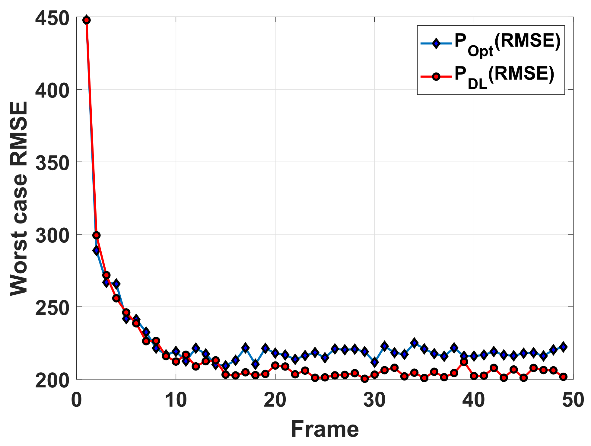
The comparison is shown in Figure 5, in which the curves labeled “ P Opt RMSE ” and “ P DL RMSE ” represent the tracking RMSEs averaged over 50 trails achieved with the optimization-based power allocation method, and proposed power allocation method, respectively. The curves labeled “ P Opt BCRLB ” and “ P DL BCRLB ” are the corresponding tracking BCRLBs. It can be seen that the tracking of the worst RMSEs are approaching the corresponding worst BCRLBs along with the number of measurements increasing. From the about 20th frame, the performance of the proposed method is about 10% higher than that of the optimization-based method with the CV model.
The estimation RMSEs and the corresponding power allocation results are presented in Figure 6 and Figure 7, respectively. In Figure 6a, the power allocation solution given by the proposed method makes the tracking RMSEs of different targets closer than that of the optimization-based method, which implies the resource utilization efficiency of the power allocation solution based on the learned policy (shown in Figure 7a) is higher than that of the optimization-based method with the CV model (shown in Figure 7b). In other words, there is room for the solution given by optimization-based method to continue to be optimized.
In Figure 7a,b, it can be seen that more power and beam resource tend to be allocated to targets that are moving away from radar, i.e., target 4, target 5, target 6, and target 7, for achieving a larger gain of tracking performance. Actually, the resource allocation is not only determined by targets’ radial distances but also by radius speeds, especially when the targets are close enough. As shown in Figure 7a, comparing the allocation results of these targets that are approaching the radar, e.g., Target 1, Target 2, Target 3, and Target 8, we discover that more power tends to be allocated to the beam pointing to the closer Target 1 because Target 1’s larger radial speeds may cause a larger BCRLB. When using the CV model for prediction, the beam selection and the power allocation are mainly determined by comparing the radius distances of different targets. For example, for the resource allocation solution of Target 1, Target 2, Target 3 shown in Figure 7b, more power and beam resources tend to be allocated to the farther targets, Target 1 and Target 2, from about frame 20. Therefore, we believe the proposed method can provide more accuracy prior information of targets, which benefits the utilization effectiveness of resource allocation.
To better illustrate the effectiveness of the RNN-based prediction network, an additional simulation experiment is conducted, where the optimization-based method is used to solve cost function (5) based on the prior information representation derived from the prediction network. In Figure 8, the curve labeled “ P Opt RNN RMSE ” represents the worst case tracking RMSE of the RNN-optimization-based method. It can be seen that this curve almost coincides with that of the proposed data-driven method and is also higher than that of the optimization-based method. This shows that the cost function (5) can be optimally solved with the method in [14] once a one-step predictive state is accurate enough. According to the comparison shown in Figure 8, it is known that, as γ = 0 , the tracking performance improvements brought from the proposed method are mainly due to the usage of the RNN-based prediction network.
Furthermore, a prediction performance comparison of the RNN-based prediction network and the Kalman filter is given in Figure 9, where the power is fixed during tracking. We first compare the RMSE of the predictive state of Target 2 (doing left turns) with the RNN and Kalman filter. The results are shown in Figure 9a, in which the prediction performance of RNN is higher than that of Kalman filter with the CV model because the model mismatch problem is avoided to a certain extent. Additionally, Figure 9b shows a comparison of the two methods of Target 3 (doing uniform linear motion). Here, Target 3 is taken in order to avoid the influence of model-mismatch. It can be seen that, different from that of Target 2, the RMSE curves of the two methods almost coincide, which implies that the performance of the RNN-based prediction network is very close (almost the same) to that of the Kalman filter with the true model (CV model), and thus, we believe that the RNN-based prediction network is able to replace the model-based prediction for target tracking in the applications of radar system resource allocation.
Next, we discuss the two methods with given RCS models. The amplitude sequences of RCS are given in Figure 10. In Figure 11, the curves labeled “ P Opt RMSE ” and “ P DL RMSE ” are the worst tracking RMSEs averaged over 50 trails achieved with the optimization-based method and the proposed method, respectively. Similar to that in the first case, the tracking performance of the proposed data-driven-based method is also superior to that of the optimization-based method. In Figure 12 and Figure 13, we present the tracking RMSE and the corresponding resource allocation results of each target with the two methods. In Figure 12, the tracking RMSE curves of targets given by the proposed method is closer than that of the optimization-based method. This indicates that the resource utilization efficiency of the optimization-based method is lower than that of the proposed method. Comparing the resource allocation results of Target 1, Target 2 and Target 3 in Figure 13a, we observe that the revisit frequency of radar for Target 3 is higher than that of the other two. This phenomenon can be explained in that a high revisit frequency benefits the tracking performance improvement of the targets with a larger radial speed. On the other hand, more power and beam resource tend to be allocated to these targets with smaller RCS amplitude, i.e., Target 1, Target 2 and Target 3, which aim to improve SNR of echoes such that the worst-case tracking performance among multiple targets is maximized.
Simulation 2: In this section, we investigate the effect of the discounted factor γ on the resource allocation results and the tracking performance. Theoretically, taking cumulative discounted tracking accuracy into the resource allocation problem is more reasonable, especially as maneuvering targets are involved. Without loss of generality, three conditions are discussed, i.e., γ = 0 , γ = 0.5 and γ = 0.99 . The target parameters are set the same as that in simulation 1 and the amplitude of the target reflectivity is also set to 1.
The worst-case tracking RMSEs with different γ are shown in Figure 14, where the result with γ = 0.99 is lower than that with γ = 0 and γ = 0.5 at the beginning, and later surpasses them with frame number increasing. This phenomenon is consistent with that the discounted factor controls the importance of the future tracking accuracy on the current resource allocation solution. Particularly, if taking a small discounted factor, the learned policy tends to improve the performance of the nearer future tracking time step at a cost of a performance loss of the farther future tracking time. In Figure 15, the tracking RMSE curves with γ = 0.5 are more compact than that with γ = 0.99 before frame 30 in order to reduce the worst-case tracking RMSE of the nearer future tracking time, which is the opposite after frame 30. The corresponding resource allocation results are presented in Figure 16. In Figure 16a, more power and beam resource are allocated to the beam pointing to target 4, target 5, target 6, and target 7, which are moving away from radar such that a larger gain of future tracking performance can be achieved. Meanwhile, increasing the revisit frequency of Target 3 aims to preventing from future larger BCRLB due to its larger radial speeds, which is the same as the result of γ = 0 . By comparing the tracking performance curves in Figure 14, it is easy to see that the tracking RMSE curves of non-zero discounted factors are lower than that of γ = 0 within frame [30, 50], which indicates that the usage of non-zero discounted factors makes the resource allocation policy improve the performance of farther tracking time. In this case, as shown in Figure 16b, in order to improve the worst-case tracking RMSE of farther tracking time as γ = 0.99 , Target 7 (it moves away from the radar with the largest radial speed) is illuminated all the time even at the beginning of tracking, and takes up most of the power at the end of tracking. This phenomenon is different from the results with γ = 0 that cares more about nearer future tracking performance.
In all, the usage of a larger γ contributes to a more stable and effective allocation policy in the case of considering farther future tracking performance. However, in this case, a performance loss of the early tracking stage would not be avoided. In other words, there is a trade-off between the current tracking performance and the future tracking performance about γ .

6. Discussion

This paper focuses on the problem of radar power allocation for multi-target tracking from a new perspective. A novel cognitive resource allocation framework is established based on deep learning. Experimental results show that the proposed method is suitable for applications that need to balance the long-term and short-term multi-target tracking performance under limited resources. In practical applications, such as tracking aircraft or missiles, targets often maneuver during tracking process, and the motion models are always unknown due to uncertainty of target motion [8,31]. In this case, the usual way is to use alternative models [32,33], such as CV and CA, for target information prediction including target position, RCS and BCRLB. However, there is a large prediction error in the prediction stage due to the existing model mismatch, which will reduce the resource allocation performance and target tracking performance. Compared with the model-optimization-based methods, the proposed data-driven method can avoid the usage of an alternative model in the prediction stage, and provide more reliable target information for resource allocation. The adoption of the combination of RNN and DRL is able to make the radar system more flexible, intelligent and forward-looking. On the other hand, since the deep-learning-based method does not need to have specific optimization methods for specific problems, we believe that this kind of data-driven method is able to solve most types of radar resource allocation problems in target tracking, such as resource allocation in scenarios of multiple maneuvering target tracking, the resource allocation considering short-term tracking effect or long-term tracking effect, and resource allocation for multiple radar system (MRS).
Our future work will mainly focus on following two aspects:
(1)
Establishing a richer maneuvering dataset. In the simulation experiments of this work, in addition to the uniform motion, the motion dataset of the prediction network also contains the data of some common maneuvering models, such as left-turn motion, right-turn motion, uniform acceleration motion, and so on. However, in real applications, the target maneuvering pattern could be more complex, and there may be the problem of target missing and the association of multiple targets. Therefore, the establishment of a more complete maneuvering target dataset is very important for a cognitive radar system.
(2)
Integrating various types of resource allocation networks and establishing a more intelligent resource allocation system. In theory, the cognitive resource allocation framework based on deep learning proposed in this paper can be used for resource allocation in many scenarios. However, resource allocation networks still need to be trained for different scenarios and different requirements, respectively, such as the scenarios with different target numbers and radar numbers. In practical applications, scenarios and requirements may change rapidly, and thus, the resource allocation strategy needs to be adjusted in real time. How to make the radar system intelligently select the appropriate resource allocation network with the changing of the scenarios and the requirements is of great significance. In our future work, the aim is to unify various types of resource allocation networks to establish an organic system and make the resource allocation process more intelligent.

7. Conclusions

In this paper, a data-driven JBSPA method for MTT is proposed and the simulation results have demonstrated its superiority. There are two keys to enhancing the MTT performance and the resource utilization efficiency, one is using the LSTM-GMM for target information prediction, which provides a reliable prior information for resource allocation, the other one is forming an MDP of resource allocation and solving with the DRL, which realizes complicate resource allocation considering long-term tracking performance. In summary, this method integrates the decision-making ability of DRL and the memory and prediction ability of RNN to make the resource allocation more flexible and further improve the cognitive ability of the radar system.

Author Contributions

Conceptualization, Y.S.; methodology, Y.S.; software, Y.S. and H.Z.; validation, Y.S. and K.L.; investigation, H.Z.; writing—original draft preparation, Y.S.; writing—review and editing, K.L.; supervision, Y.S. All authors have read and agreed to the published version of the manuscript.

Funding

This work was supported by the Fund for Foreign Scholars in University Research and Teaching Programs (the 111 Project) (No. B18039), Shaanxi Innovation Team Project.

Data Availability Statement

Not applicable.

Conflicts of Interest

The authors declare no conflict of interest.

References

  1. Blackman, S. Multiple-Target Tracking with Radar Applications; Artech House: Norwood, MA, USA, 1986. [Google Scholar]
  2. Stone, L.D.; Barlow, C.A.; Corwin, T. Bayesian Multiple Target Tracking; Artech House: Norwood, MA, USA, 1999. [Google Scholar]
  3. Hue, C.; Cadre, J.L.; Pérez, P. Sequential Monte Carlo methods for multiple target tracking and data fusion. IEEE Trans. Signal Process. 2002, 50, 309–325. [Google Scholar] [CrossRef] [Green Version]
  4. Stoica, P.; Li, J. MIMO radar with colocated antennas. IEEE Signal Process. Mag. 2007, 24, 106–114. [Google Scholar]
  5. Gorji, A.A.; Tharmarasa, R.; Blair, W.D.; Kirubarajan, T. Multiple unresolved target localization and tracking using collocated MIMO radars. IEEE Trans. Aerosp. Electron. Syst. 2012, 48, 2498–2517. [Google Scholar] [CrossRef]
  6. Rabideau, D.J.; Parker, P. Ubiquitous MIMO Multifunction Digital Array Radar and the Role of Time-Energy Management in Radar; Project Rep. DAR-4; MIT Lincoln Lab.: Lexington, MA, USA, 2003. [Google Scholar]
  7. Godrich, H.; Petropulu, A.P.; Poor, H.V. Power allocation strategies for target localization in distributed multiple-radar architecture. IEEE Trans. Signal Process. 2011, 59, 3226–3240. [Google Scholar] [CrossRef]
  8. Chavali, P.; Nehorai, A. Scheduling and power allocation in a cognitive radar network for multiple-target tracking. IEEE Trans. Signal Process. 2012, 50, 715–729. [Google Scholar] [CrossRef]
  9. Yan, J.; Dai, J.; Pu, W.; Zhou, S.; Liu, H.; Bao, Z. Quality of service constrained-resource allocation scheme for multiple target tracking in radar sensor network. IEEE Syst. J. 2021, 15, 771–779. [Google Scholar] [CrossRef]
  10. Haykin, S.; Zia, A.; Arasaratnam, I.; Yanbo, X. Cognitive tracking radar. In Proceedings of the 2010 IEEE Radar Conference, Washington, DC, USA, 10–14 May 2010.
  11. Tichavsky, P.; Muravchik, C.H.; Nehorai, A. Posterior Cramér-Rao bounds for discrete-time nonlinear filtering. IEEE Trans. Signal Process. 1998, 46, 1386–1396. [Google Scholar] [CrossRef] [Green Version]
  12. Hernandez, M.; Kirubarajan, T.; Bar-Shalom, Y. Multisensor resource deployment using posterior Cramér-Rao bounds. IEEE Trans. Aerosp. Electron. Syst. 2004, 40, 399–416. [Google Scholar] [CrossRef]
  13. Hernandez, M.L.; Farina, A.; Ristic, B. PCRLB for tracking in cluttered environments: Measurement sequence conditioning approach. IEEE Trans. Aerosp. Electron. Syst. 2006, 42, 680–704. [Google Scholar] [CrossRef]
  14. Yan, J.; Liu, H.; Jiu, B.; Chen, B.; Liu, Z.; Bao, Z. Simultaneous multibeam resource allocation scheme for multiple target tracking. IEEE Trans. Signal Process. 2015, 63, 3110–3122. [Google Scholar] [CrossRef]
  15. Shi, Y.; Jiu, B.; Yan, J.; Liu, H.; Wang, C. Data-driven simultaneous multibeam power allocation: When multiple targets tracking meets deep reinforcement learning. IEEE Syst. J. 2021, 15, 1264–1274. [Google Scholar] [CrossRef]
  16. Cormode, G.; Thottan, M. Algorithms for Next Generation Networks; Springer: London, UK, 2010. [Google Scholar]
  17. Hochreiter, S.; Schmidhuber, J. Long Short-Term Memory. Neural Comput. 1997, 9, 1735–1780. [Google Scholar] [CrossRef] [PubMed]
  18. Mnih, V.; Kavukcuoglu, K.; Silver, D.; Rusu, A.A.; Veness, J.; Bellemare, M.G.; Graves, A.; Riedmiller, M.; Fidjeland, A.K.; Ostrovski, G.; et al. Human-level control through deep reinforcement learning. Nature 2015, 518, 529–533. [Google Scholar] [CrossRef] [PubMed]
  19. Sutton, R.S.; Barto, A.G. Reinforcement Learning: An Introduction, 2nd ed.; MIT Press: Cambridge, MA, USA, 2018. [Google Scholar]
  20. Shi, Y.; Jiu, B.; Yan, J.; Liu, H. Data-Driven radar selection and power allocation method for target tracking in multiple radar system. IEEE Sens. J. 2021, 21, 19296–19306. [Google Scholar] [CrossRef]
  21. Lillicrap, T.P.; Hunt, J.J.; Pritzel, A.; Heess, N.; Erez, T.; Tassa, Y.; Silver, D.; Wierstra, D. Continuous control with deep reinforcement learning. In Proceedings of the 4th International Conference on Learning Representations, San Juan, Puerto Rico, 2–4 May 2016. [Google Scholar]
  22. Silver, D.; Lever, G.; Heess, N.; Degris, T.; Wierstra, D.; Riedmiller, M. Deterministic policy gradient algorithms. In Proceedings of the 31st International Conference on Machine Learning, Beijing, China, 21–26 June 2014. [Google Scholar]
  23. Sutton, R.S.; McAllester, D.A.; Singhand, S.P.; Mansour, Y. Policy gradient methods for reinforcement learning with function approximation. In Proceedings of the 12th IInternational Conference on Neural Information Processing Systems, Denver, CO, USA, 27–30 November 2000. [Google Scholar]
  24. Van Trees, H.L. Detection, Estimation, and Modulation Theory, Part III; Wiley: New York, NY, USA, 1971. [Google Scholar]
  25. Van Trees, H.L. Optimum Array Processing: Detection, Estimation, and Modulation Theory, Part IV; Wiley: New York, NY, USA, 2002. [Google Scholar]
  26. Niu, R.; Willett, P.; Bar-Shalom, Y. Matrix CRLB scaling due to measurements of uncertain origin. IEEE Trans. Signal Process. 2001, 49, 1325–1335. [Google Scholar]
  27. Zhang, X.; Willett, P.; Bar-Shalom, Y. Dynamic Cramer-Rao bound for target tracking in clutter. IEEE Trans. Aerosp. Electron. Syst. 2005, 41, 1154–1167. [Google Scholar] [CrossRef]
  28. Stocia, P.; Selén, Y. Cyclic minimizer, majorization techniques, and expectation-maximization algorithm: A refresher. IEEE Signal Process. Mag. 2004, 21, 112–114. [Google Scholar]
  29. Kingma, D.; Ba, J. Adam: A method for stochastic optimization. Proceedings of the 3rd International Conference for Design. In Proceedings of the 3rd International Conference for Design, Santiago de Chile, Chile, 28–30 June 2015. [Google Scholar]
  30. Ristic, B.; Arulampalam, S.; Gordon, N. Beyond the Kalman Filter Particle Filters for Tracking Applications; Artech House: Norwell, MA, USA, 2004. [Google Scholar]
  31. Yan, J.; Pu, W.; Liu, H.; Bo, J.; Bao, Z. Robust chance constrained power allocation scheme for multiple target localization in colocated MIMO system. IEEE Trans. Signal Process. 2018, 21, 3946–3957. [Google Scholar] [CrossRef]
  32. Yan, J.; Pu, W.; Zhou, S.; Liu, H.; Bao, Z. Collaborative detection and power allocation framework for target tracking in multiple radar system. Inf. Fusion 2020, 55, 178–183. [Google Scholar] [CrossRef]
  33. Yan, J.; Pu, W.; Zhou, S.; Liu, H.; Greco, M.S. Optimal Resource Allocation for Asynchronous Multiple Targets Tracking in Heterogeneous Radar Network. IEEE Trans. Signal Process. 2020, 68, 4055–4068. [Google Scholar] [CrossRef]
Figure 1. The system architecture of DRL–JBSPA.
Remotesensing 14 01674 g001
Figure 2. The prediction network.
Remotesensing 14 01674 g002
Figure 3. The Actor-Critic network.
Remotesensing 14 01674 g003
Figure 4. Real moving trajectories of targets.
Remotesensing 14 01674 g004
Figure 5. The worst case RMSEs achieved with different power allocation methods versus corresponding worst case BCRLBs.
Remotesensing 14 01674 g005
Figure 6. Tracking RMSEs of different targets. (a) Proposed power allocation method. (b) Optimization-based power allocation method.
Remotesensing 14 01674 g006
Figure 7. The simultaneous multibeam power allocation results. (a) Proposed power allocation method. (b) Optimization-based power allocation method.
Remotesensing 14 01674 g007
Figure 8. Worst case RMSEs achieved by the optimization-based method based on the prior representation derived by the prediction network.
Remotesensing 14 01674 g008
Figure 9. RMSE comparison of predictive state of different methods. (a) Target 2 (b) Target 1.
Remotesensing 14 01674 g009
Figure 10. RCS model.
Remotesensing 14 01674 g010
Figure 11. The worst case RMSEs.
Remotesensing 14 01674 g011
Figure 12. Tracking RMSEs of different targets with given RCS model. (a) Proposed power allocation method. (b) Optimization-based power allocation method.
Remotesensing 14 01674 g012
Figure 13. The resource allocation results. (a) Proposed power allocation method. (b) Optimization-based power allocation method.
Remotesensing 14 01674 g013
Figure 14. The worst case RMSEs with different γ .
Remotesensing 14 01674 g014
Figure 15. Tracking RMSEs of different targets. (a) γ = 0.5 (b) γ = 0.99 .
Remotesensing 14 01674 g015
Figure 16. The resource allocation results. (a) γ = 0.5 (b) γ = 0.99 .
Remotesensing 14 01674 g016
Table 1. Target motion parameters.
Motion ModeTurning FrequencyInitial Velocity
Target 1Right-turn motion0.0035 200 m / s , 200 m / s
Target 2Left-turn motion0.0035 200 m / s , 200 m / s
Target 3Uniform linear motion* 200 m / s , 200 m / s
Target 4Right-turn motion0.0035 200 m / s , 200 m / s
Target 5Left-turn motion0.0035 200 m / s , 200 m / s
Target 6Uniform linear motion* 200 m / s , 200 m / s
Target 7Uniform linear motion* 200 m / s , 200 m / s
Target 8Left-turn motion0.0035 200 m / s , 200 m / s
Publisher’s Note: MDPI stays neutral with regard to jurisdictional claims in published maps and institutional affiliations.

