
Detection of Grassland Mowing Events for Germany by Combining Sentinel-1 and Sentinel-2 Time Series

 , , ,
, , ,
Abstract
:
1. Introduction
2. Materials
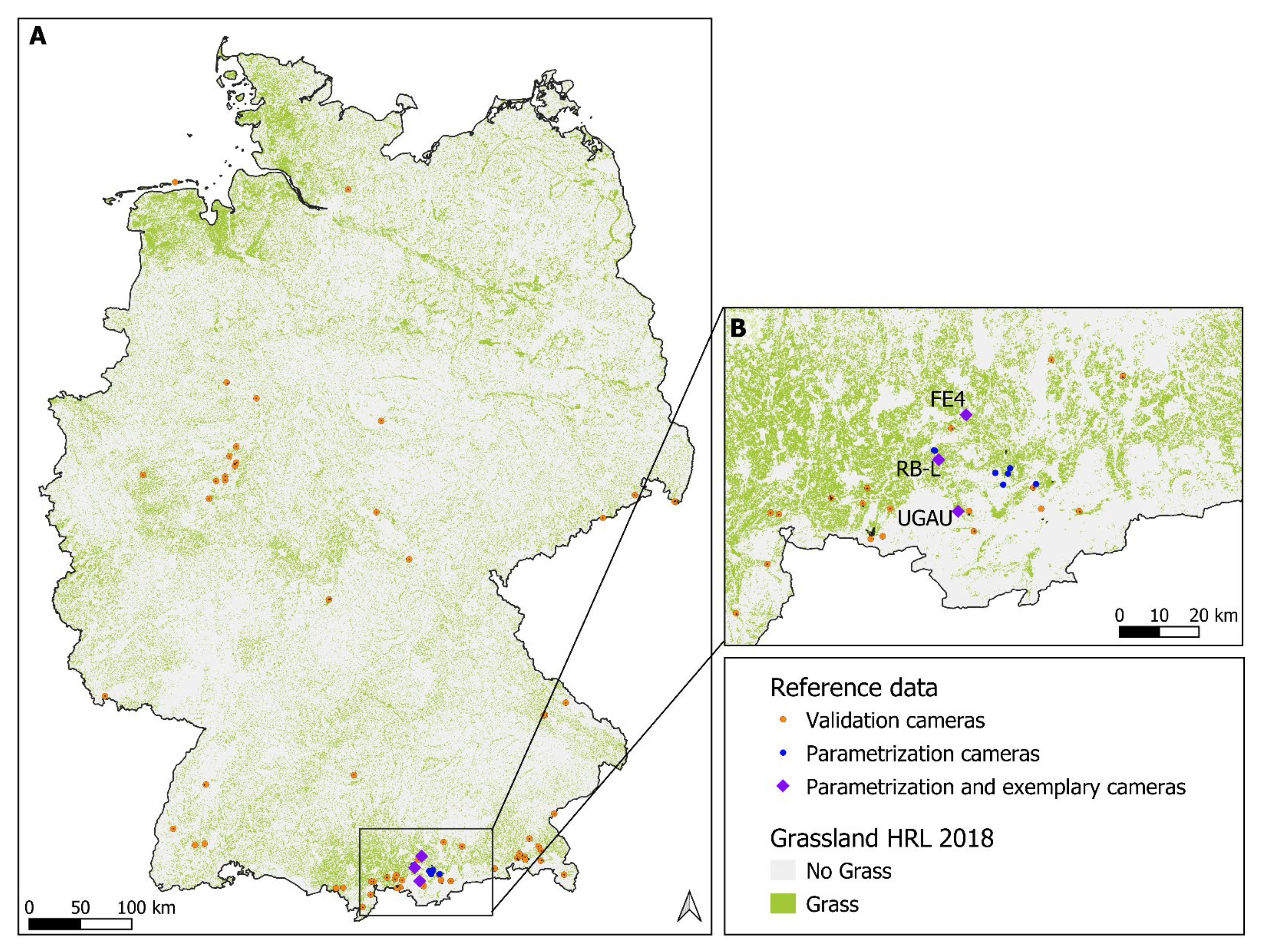
2.1. Study Area
2.1.1. Germany
2.1.2. Focus Region
2.2. Ground Data
2.2.1. Parametrization Data
2.2.2. Validation Data for National Mowing Event Detection
2.2.3. Validation Data for the Mowing Event Detection in the Focus Region
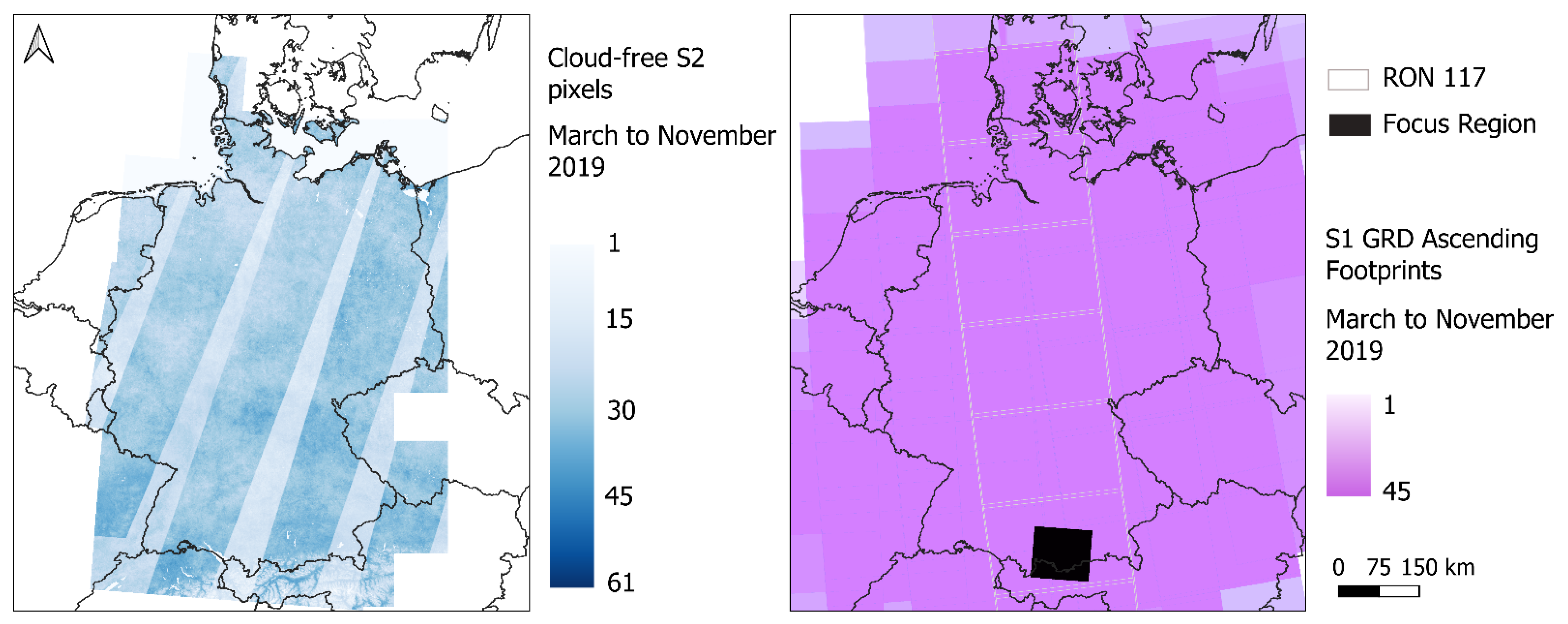
2.3. Satellite Data
3. Methods
3.1. Pre-Processing of Satellite Data
3.1.1. Pre-Processing of Sentinel-2 Data
3.1.2. Pre-Processing of Sentinel-1 Data
3.2. Mowing Detection Approach Development
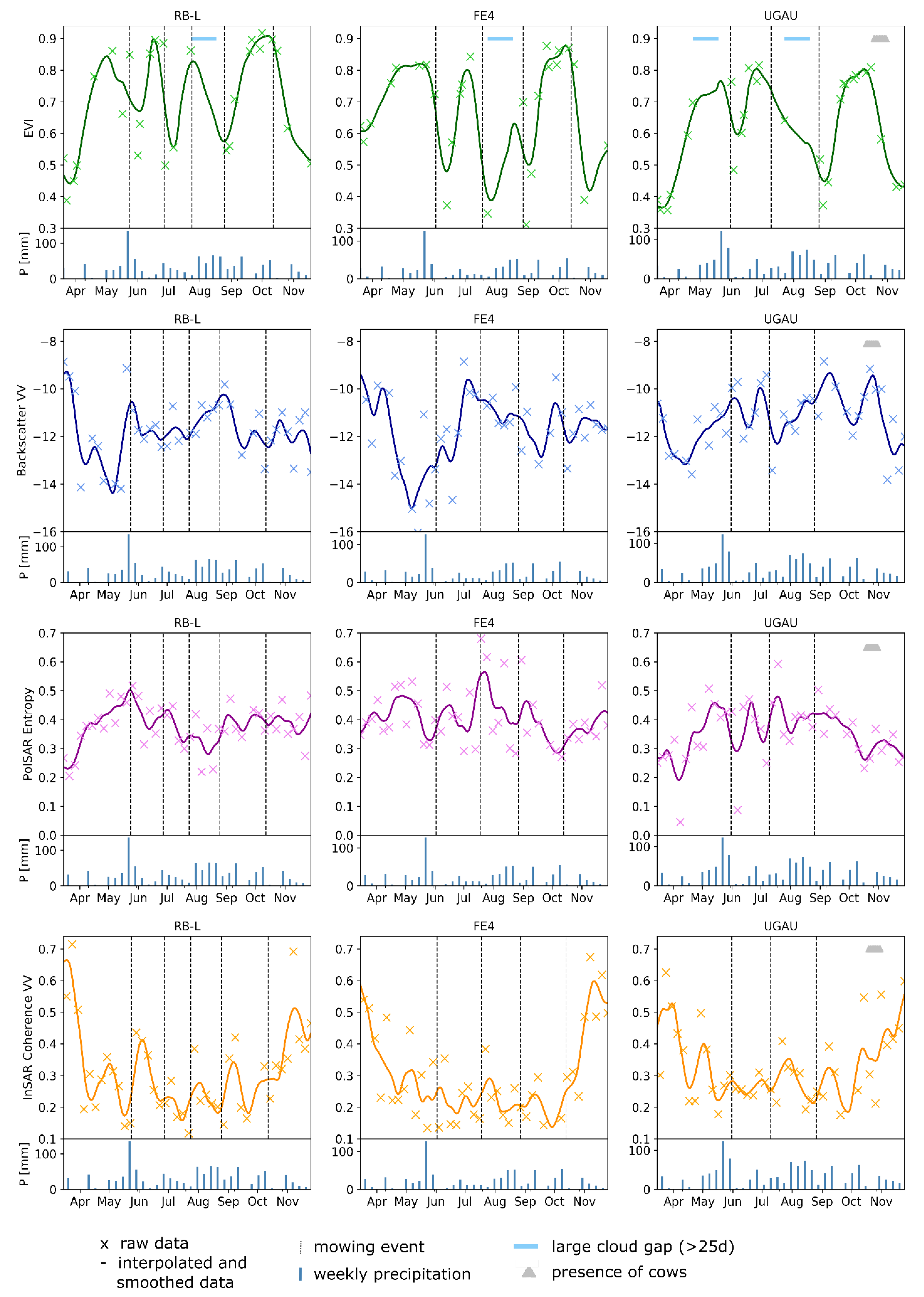
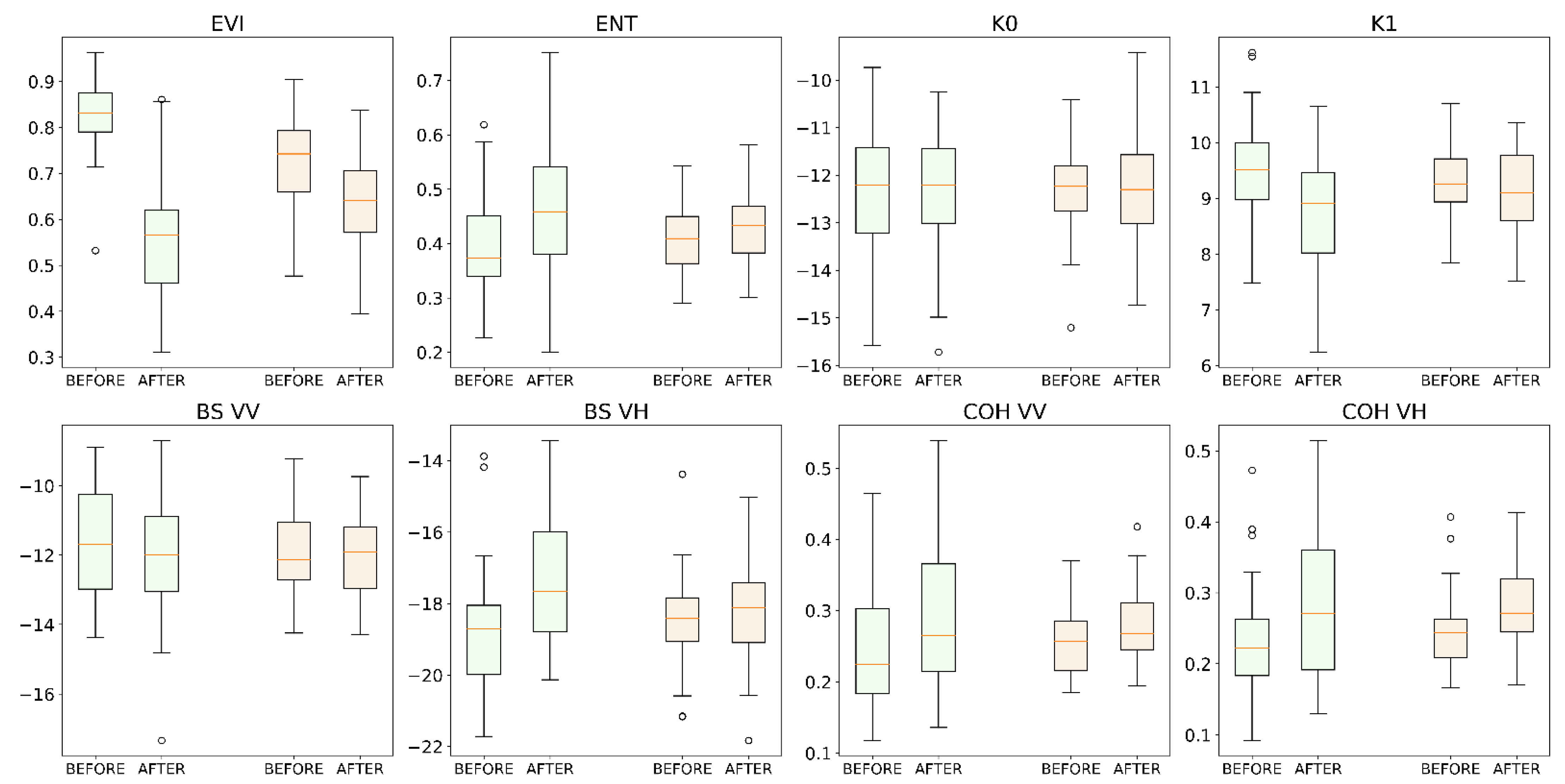
3.2.1. Investigation of Satellite Time Series and Variable Selection
3.2.2. Rule-Set Development and Parametrization
EVI-Based Mowing Detection Algorithm
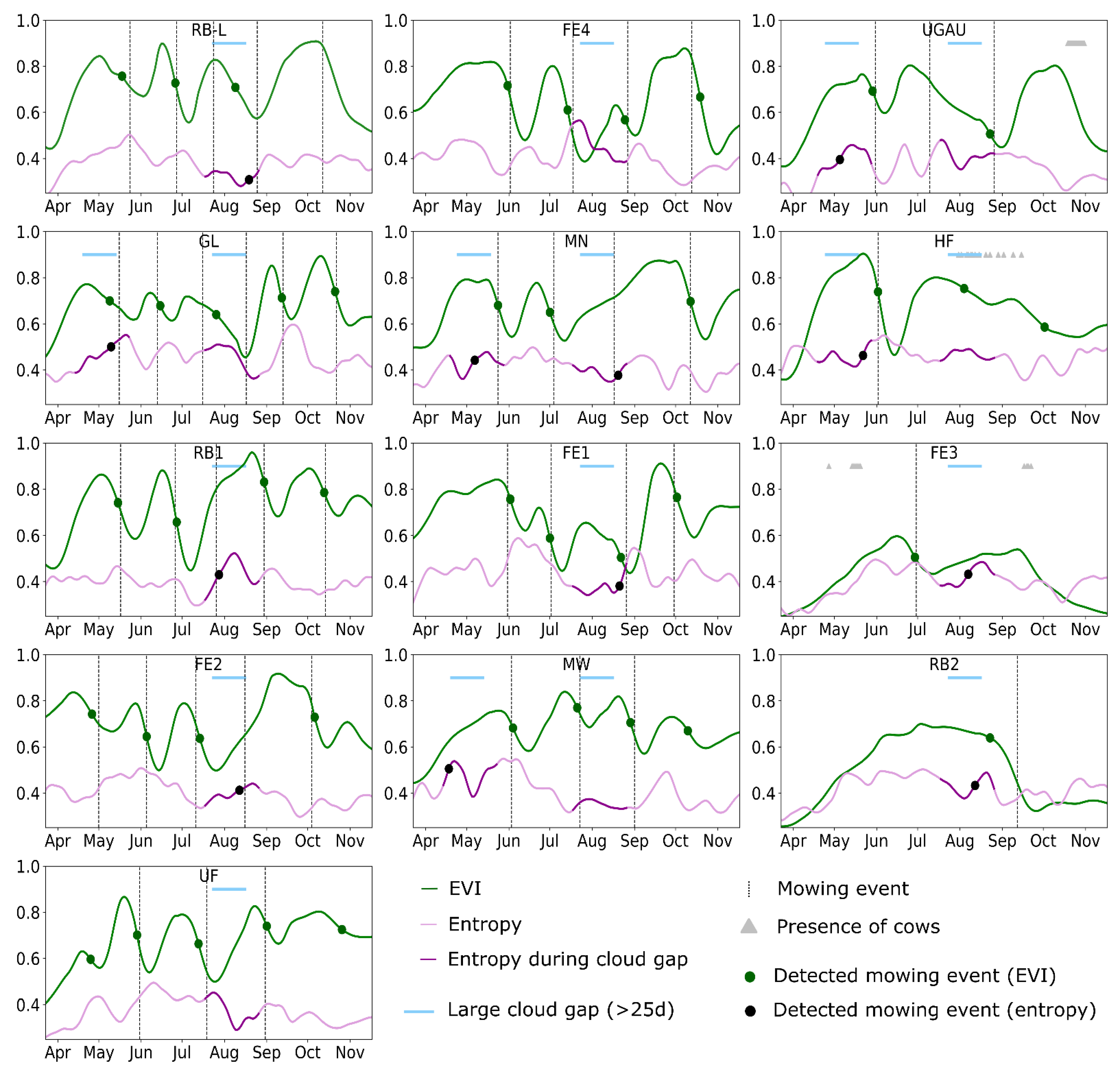
EVI + Entropy-Based Mowing Detection
3.3. Validation Procedure
3.3.1. Validation Procedure for the Detection of Grassland Mowing Events
3.3.2. Accuracy Assessment of the Mowing Event Detection
3.4. Uncertainty Information
4. Results
4.1. Accuracy Assessment on Parametrization Sites
4.1.1. EVI-Based Mowing Detection Algorithm
4.1.2. EVI + Entropy-Based Mowing Detection
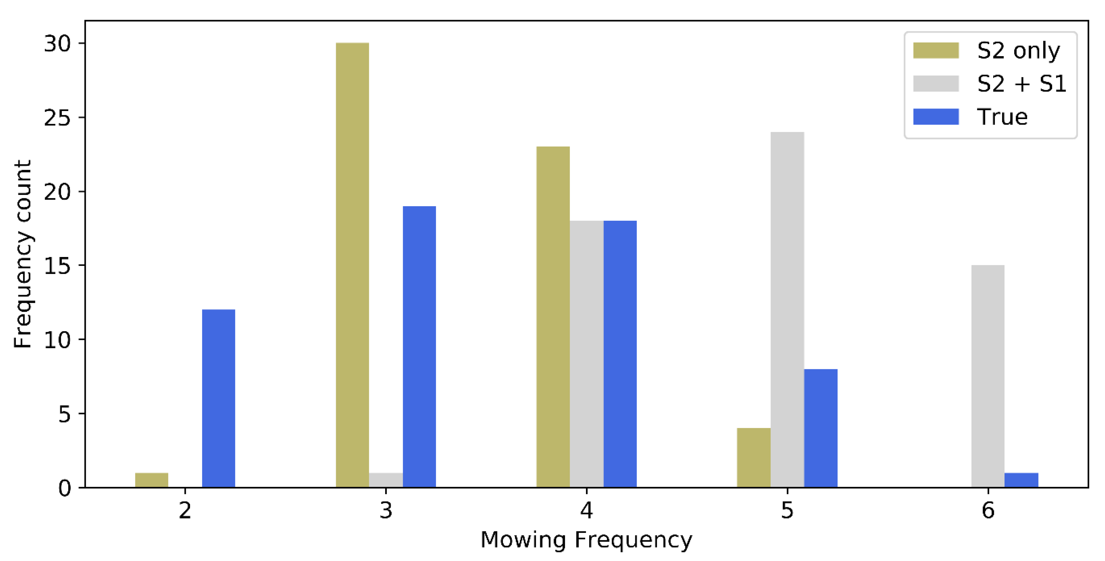
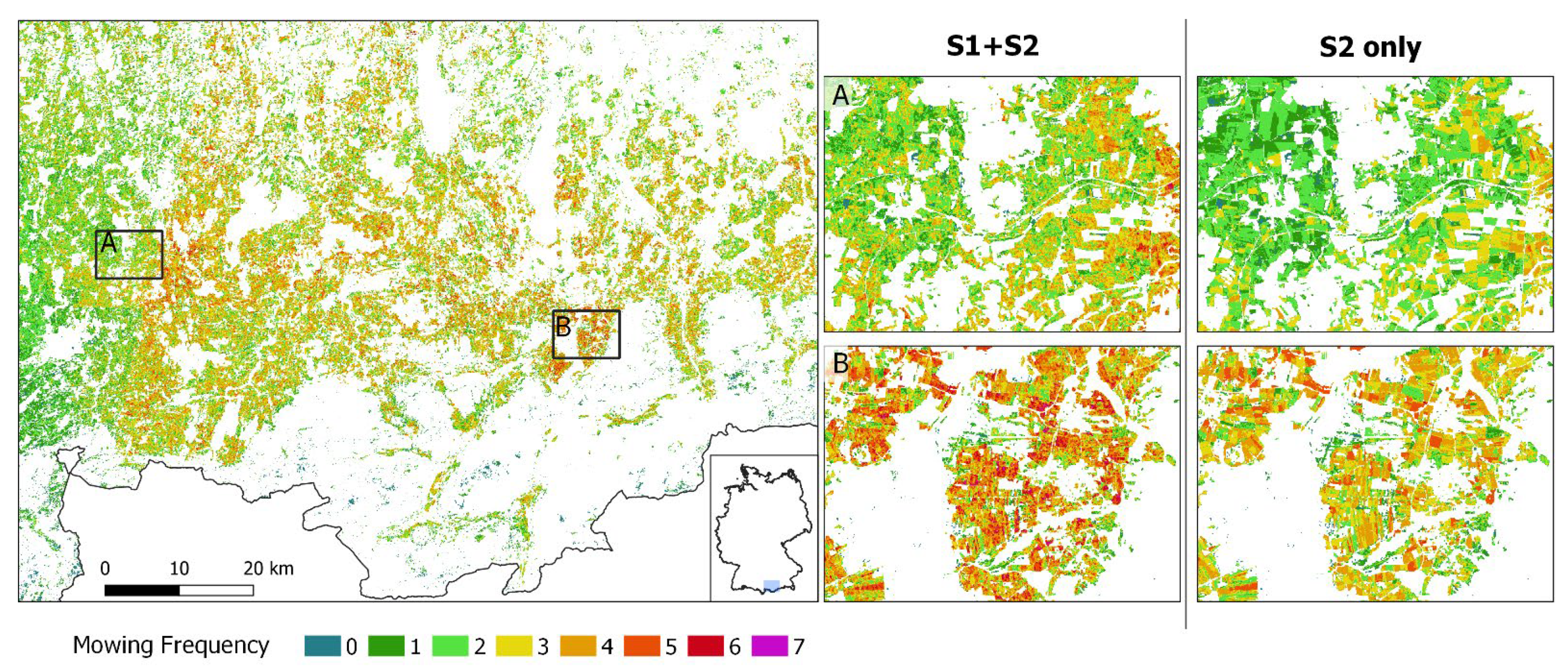
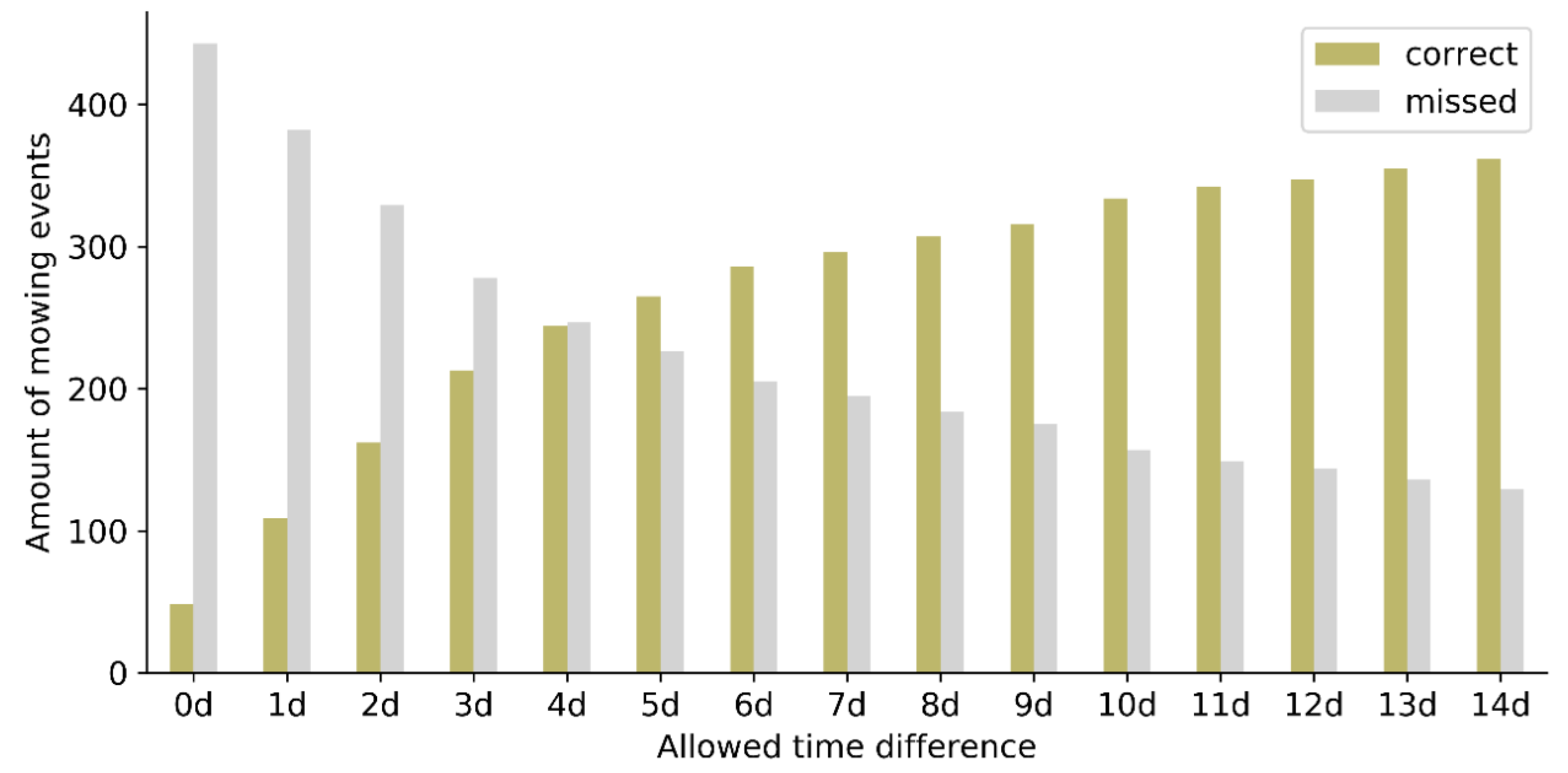
4.2. Mowing Detection Validation of the Focus Region
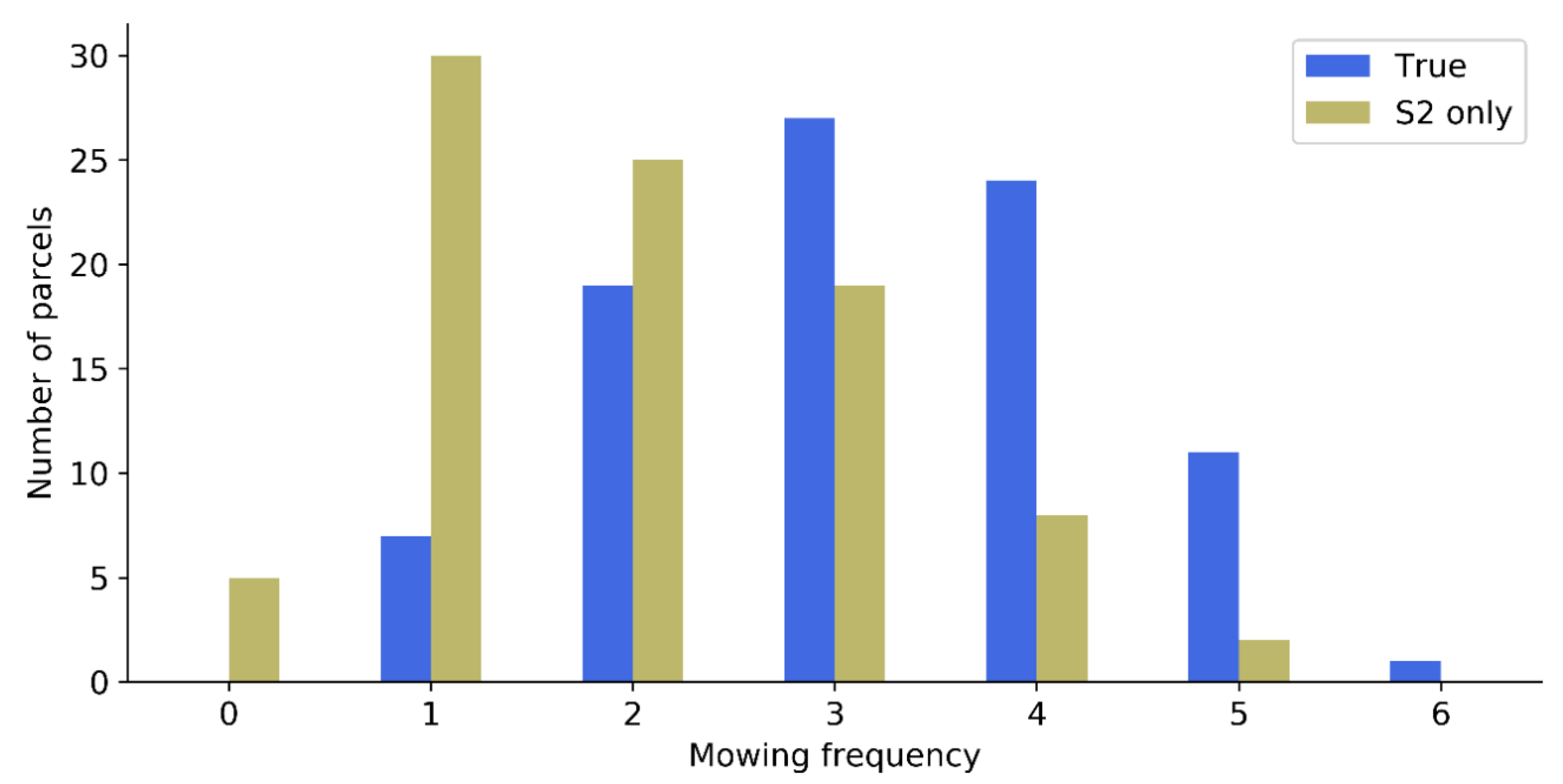
4.3. Germany-Wide Validation of S2-Based Mowing Detection
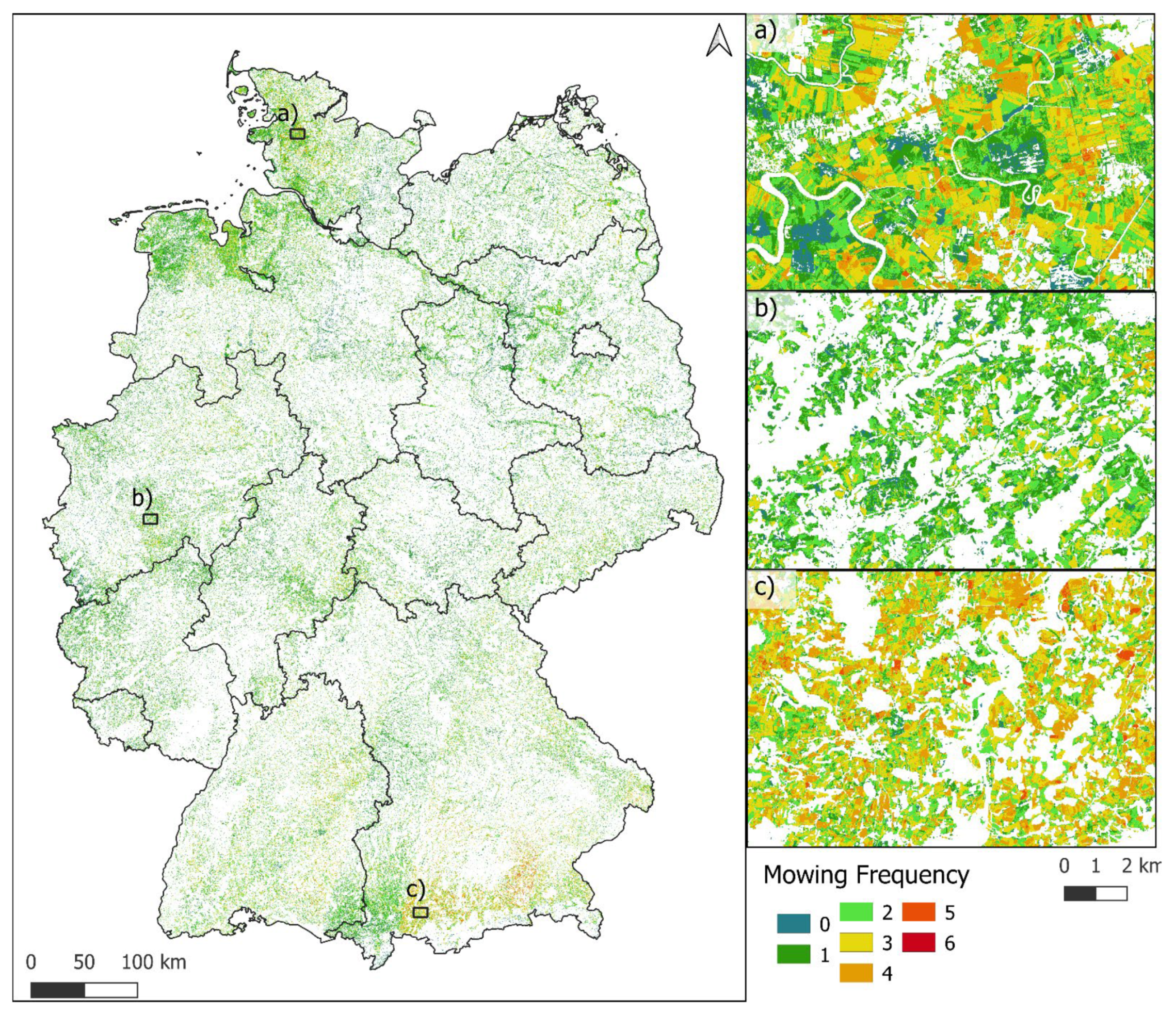
4.4. Germany-Wide Application of S2-Based Mowing Event Detection
5. Discussion
5.1. Relationships between S1 and S2 Parameters and Mowing Events
5.1.1. The Relationship of S2-Based EVI to Mowing Events
5.1.2. The Relationship of S1-Based Backscatter to Mowing Events
5.1.3. The Relationship of S1-Based InSAR Coherence to Mowing Events
5.1.4. The Relationship of S1-Based PolSAR Decomposition Parameters to Mowing Events
5.2. Spatial Patterns of Detected Mowing Events in Germany
5.3. Importance and Drawbacks of Optical and SAR Data Fusion
6. Conclusions
- The detection of grassland mowing events is possible with optical data; however, only if dense time (period < 10 to 14 days) series are available;
- A pixel-based approach is possible and advantageous as parcels are at times not used homogenously;
- The temporal signal of InSAR and PolSAR parameters for mown grasslands are inconsistent and do not reveal a clear relation to mowing events. Most probably they depend on additional drivers (i.e., moisture), for which general assumptions are difficult to make;
- Complementing the optical mowing detection approach based on EVI time series by the PolSAR entropy, led to an increase in detected mowing events by 9.2%. However, more false positives also occurred, resulting in a drop of the F1-Score (F1-Score = 0.65 for S2 only, F1-Score = 0.61 for S2 + S1);
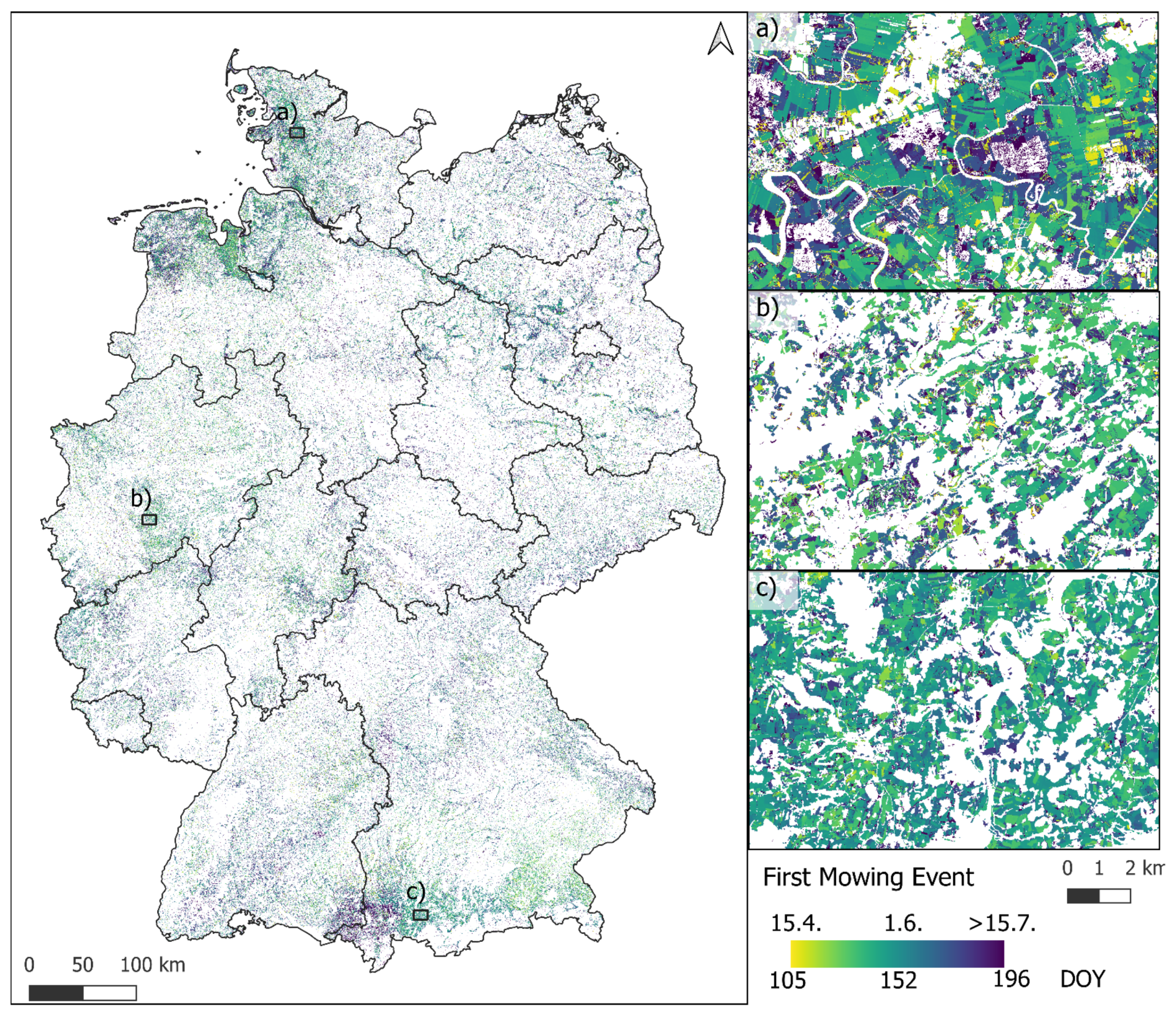
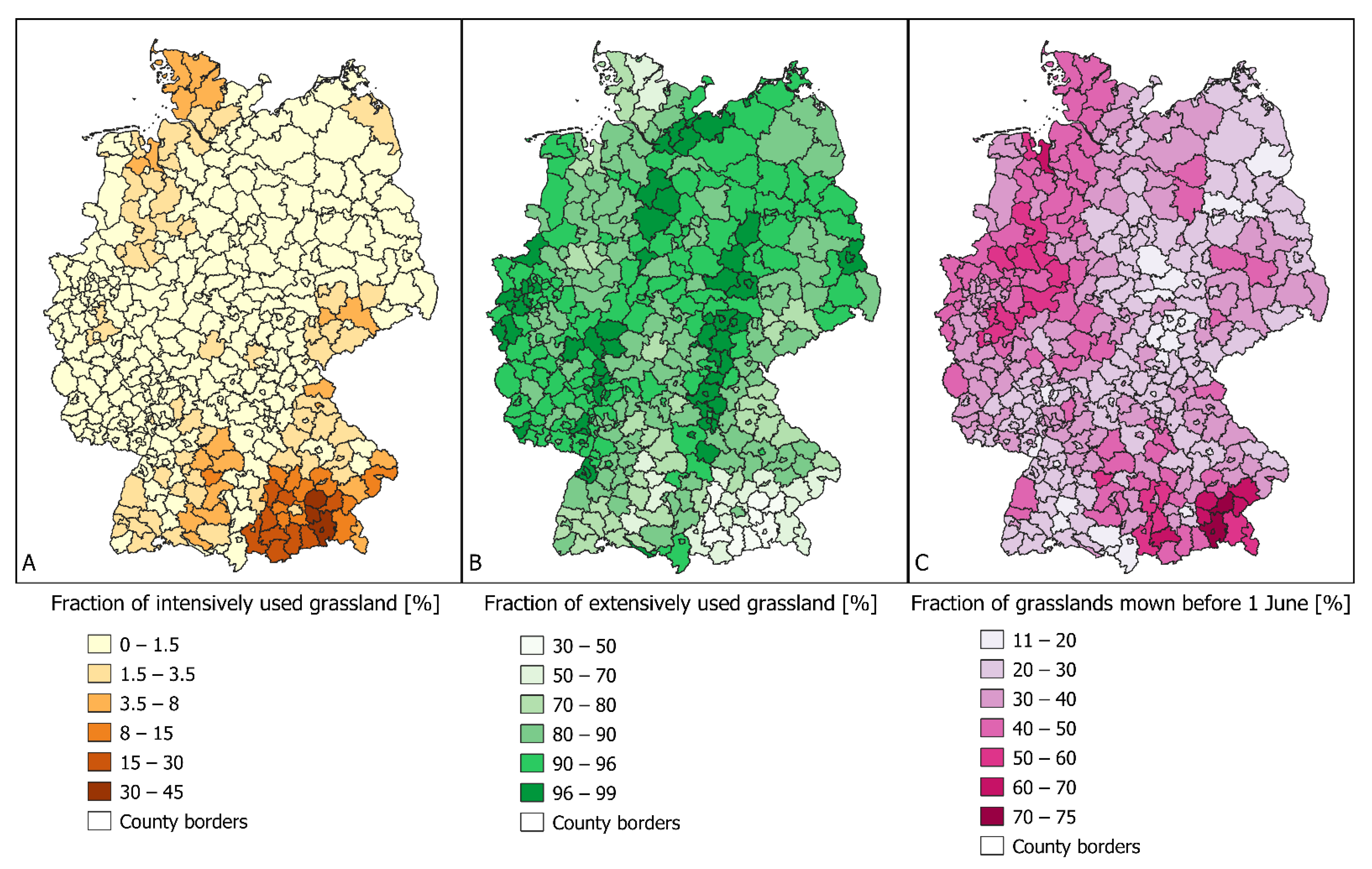
- Use intensity and timing of the first mowing event of grasslands in Germany are heterogeneously distributed with more often mown parcels in the south/south-east and the north;
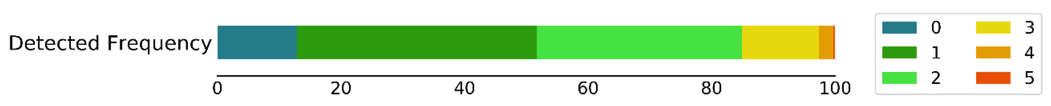
- In Germany, 13% of grasslands are not mown at all and a majority is only mown one (38%) to two times (33%), which might be grazed as well. Only 3% of all grasslands are mown four to six times, according to our analysis.
Supplementary Materials
Author Contributions
Funding
Data Availability Statement
Acknowledgments
Conflicts of Interest
References
- Reynolds, S.; Frame, J. Grasslands: Developments, Opportunities, Perspectives; Food & Agriculture Organization: Rome, Italy, 2005. [Google Scholar]
- White, R.P.; Murray, S.; Rohweder, M. Pilot Analysis of Global Ecosystems—Grassland Ecosystems; World Resources Institute: Washington, DC, USA, 2000. [Google Scholar]
- Bengtsson, J.; Bullock, J.M.; Egoh, B.; Everson, C.; Everson, T.; O’Connor, T.; O’Farrell, P.J.; Smith, H.G.; Lindborg, R. Grasslands-more important for ecosystem services than you might think. Ecosphere 2019, 10, e02582. [Google Scholar] [CrossRef]
- Schoof, N.; Luick, R.; Ackermann, A.; Baum, S.; Böhner, H.; Röder, N.; Rudolph, S.; Schmidt, T.G.; Hötker, H.; Jeromin, H. (Eds.) Auswirkungen der Neuen Rahmenbedingungen der Gemeinsamen Agrarpolitik Auf Die Grünland-Bezogene Biodiversität, 2nd ed.; BfN-Skripten; Bundesamt für Naturschutz: Bonn, Germany, 2020; Volume 540, ISBN 978-3-89624-278-5. [Google Scholar]
- Poeplau, C.; Jacobs, A.; Don, A.; Vos, C.; Schneider, F.; Wittnebel, M.; Tiemeyer, B.; Heidkamp, A.; Prietz, R.; Flessa, H. Stocks of organic carbon in German agricultural soils—Key results of the first comprehensive inventory. J. Plant Nutr. Soil Sci. 2020, 183, 665–681. [Google Scholar] [CrossRef]
- Dengler, J.; Janišová, M.; Török, P.; Wellstein, C. Biodiversity of Palaearctic grasslands: A synthesis. Agric. Ecosyst. Environ. 2014, 182, 1–14. [Google Scholar] [CrossRef] [Green Version]
- Zhang, Y.; Loreau, M.; He, N.; Zhang, G.; Han, X. Mowing exacerbates the loss of ecosystem stability under nitrogen enrichment in a temperate grassland. Funct. Ecol. 2017, 31, 1637–1646. [Google Scholar] [CrossRef] [Green Version]
- Smith, A.L.; Barrett, R.L.; Milner, R.N.C. Annual mowing maintains plant diversity in threatened temperate grasslands. Appl. Veg. Sci. 2018, 21, 207–218. [Google Scholar] [CrossRef]
- Bernhardt-Römermann, M.; Römermann, C.; Sperlich, S.; Schmidt, W. Explaining grassland biomass–the contribution of climate, species and functional diversity depends on fertilization and mowing frequency. J. Appl. Ecol. 2011, 48, 1088–1097. [Google Scholar] [CrossRef] [Green Version]
- Gilmullina, A.; Rumpel, C.; Blagodatskaya, E.; Chabbi, A. Management of grasslands by mowing versus grazing—impacts on soil organic matter quality and microbial functioning. Appl. Soil Ecol. 2020, 156, 103701. [Google Scholar] [CrossRef]
- Senapati, N.; Chabbi, A.; Gastal, F.; Smith, P.; Mascher, N.; Loubet, B.; Cellier, P.; Naisse, C. Net carbon storage measured in a mowed and grazed temperate sown grassland shows potential for carbon sequestration under grazed system. Carbon Manag. 2014, 5, 131–144. [Google Scholar] [CrossRef]
- Schoof, N.; Luick, R.; Beaufoy, G.; Jones, G.; Einarsson, P.; Ruiz, J.; Stefanova, V.; Fuchs, D.; Windmaißer, T.; Hötker, H.; et al. (Eds.) Grünlandschutz in Deutschland: Treiber der Biodiversität, Einfluss von Agrarumwelt-und Klimamaßnahmen, Ordnungsrecht, Molkereiwirtschaft und Auswirkungen der Klima-und Energiepolitik, 2nd ed.; BfN-Skripten; Bundesamt für Naturschutz: Bonn, Germany, 2020; Volume 539, ISBN 978-3-89624-277-8. [Google Scholar]
- Socher, S.A.; Prati, D.; Boch, S.; Müller, J.; Klaus, V.H.; Hölzel, N.; Fischer, M. Direct and productivity-mediated indirect effects of fertilization, mowing and grazing on grassland species richness. J. Ecol. 2012, 100, 1391–1399. [Google Scholar] [CrossRef]
- Hilpold, A.; Seeber, J.; Fontana, V.; Niedrist, G.; Rief, A.; Steinwandter, M.; Tasser, E.; Tappeiner, U. Decline of rare and specialist species across multiple taxonomic groups after grassland intensification and abandonment. Biodivers. Conserv. 2018, 27, 3729–3744. [Google Scholar] [CrossRef]
- European Commission Regulation (EU) No 1305/2013 of the European Parliament and of the Council of 17 December 2013 on support for rural development by the European Agricultural Fund for Rural Development (EAFRD) and repealing Council Regulation (EC) No 1698/2005. Off. J. Eur. Union L 2013, 347, 487–548.
- Reinermann, S.; Asam, S.; Kuenzer, C. Remote Sensing of Grassland Production and Management—A Review. Remote Sens. 2020, 12, 1949. [Google Scholar] [CrossRef]
- Schwieder, M.; Wesemeyer, M.; Frantz, D.; Pfoch, K.; Erasmi, S.; Pickert, J.; Nendel, C.; Hostert, P. Mapping grassland mowing events across Germany based on combined Sentinel-2 and Landsat 8 time series. Remote Sens. Environ. 2021, 9, 112795. [Google Scholar] [CrossRef]
- Courault, D.; Hadria, R.; Ruget, F.; Olioso, A.; Duchemin, B.; Hagolle, O.; Dedieu, G. Combined use of FORMOSAT-2 images with a crop model for biomass and water monitoring of permanent grassland in Mediterranean region. Hydrol. Earth Syst. Sci. Discuss. 2010, 14, 1731–1744. [Google Scholar] [CrossRef] [Green Version]
- Kolecka, N.; Ginzler, C.; Pazur, R.; Price, B.; Verburg, P.H. Regional Scale Mapping of Grassland Mowing Frequency with Sentinel-2 Time Series. Remote Sens. 2018, 10, 1221. [Google Scholar] [CrossRef] [Green Version]
- Griffiths, P.; Nendel, C.; Pickert, J.; Hostert, P. Towards national-scale characterization of grassland use intensity from integrated Sentinel-2 and Landsat time series. Remote Sens. Environ. 2020, 238, 111124. [Google Scholar] [CrossRef]
- Schuster, C.; Ali, I.; Lohmann, P.; Frick, A.; Foerster, M.; Kleinschmit, B. Towards Detecting Swath Events in TerraSAR-X Time Series to Establish NATURA 2000 Grassland Habitat Swath Management as Monitoring Parameter. Remote Sens. 2011, 3, 1308–1322. [Google Scholar] [CrossRef] [Green Version]
- Grant, K.; Siegmund, R.; Wagner, M.; Hartmann, S. Satellite-based assessment of grassland yields. Int. Arch. Photogramm. Remote Sens. Spat. Inf. Sci. 2015, 40, 15. [Google Scholar] [CrossRef] [Green Version]
- Taravat, A.; Wagner, M.P.; Oppelt, N. Automatic Grassland Cutting Status Detection in the Context of Spatiotemporal Sentinel-1 Imagery Analysis and Artificial Neural Networks. Remote Sens. 2019, 11, 711. [Google Scholar] [CrossRef] [Green Version]
- De Vroey, M.; Radoux, J.; Defourny, P. Grassland Mowing Detection Using Sentinel-1 Time Series: Potential and Limitations. Remote Sens. 2021, 13, 348. [Google Scholar] [CrossRef]
- Voormansik, K.; Jagdhuber, T.; Olesk, A.; Hajnsek, I.; Papathanassiou, K.P. Towards a detection of grassland cutting practices with dual polarimetric TerraSAR-X data. Int. J. Remote Sens. 2013, 34, 8081–8103. [Google Scholar] [CrossRef]
- Zalite, K.; Voormansik, K.; Praks, J.; Antropov, O.; Noorma, M. Towards Detecting Mowing of Agricultural Grasslands from Multi-Temporal COSMO-SkyMed Data; IEEE Geoscience and Remote Sensing Symposium: Quebec City, QC, Canada, 2014; pp. 5076–5079. [Google Scholar]
- Zalite, K.; Antropov, O.; Praks, J.; Voormansik, K.; Noorma, M. Monitoring of agricultural grasslands with time series of X-band repeat-pass interferometric SAR. IEEE J. Sel. Top. Appl. Earth Obs. Remote Sens. 2015, 9, 3687–3697. [Google Scholar] [CrossRef]
- Voormansik, K.; Jagdhuber, T.; Zalite, K.; Noorma, M.; Hajnsek, I. Observations of cutting practices in agricultural grasslands using polarimetric SAR. IEEE J. Sel. Top. Appl. Earth Obs. Remote Sens. 2015, 9, 1382–1396. [Google Scholar] [CrossRef]
- Ali, I.; Barrett, B.; Cawkwell, F.; Green, S.; Dwyer, E.; Neumann, M. Application of Repeat-Pass TerraSAR-X staring spotlight interferometric coherence to monitor pasture biophysical parameters: Limitations and sensitivity analysis. IEEE J. Sel. Top. Appl. Earth Obs. Remote Sens. 2017, 10, 3225–3231. [Google Scholar] [CrossRef] [Green Version]
- Tamm, T.; Zalite, K.; Voormansik, K.; Talgre, L. Relating Sentinel-1 interferometric coherence to mowing events on grasslands. Remote Sens. 2016, 8, 802. [Google Scholar] [CrossRef] [Green Version]
- Voormansik, K.; Zalite, K.; Sünter, I.; Tamm, T.; Koppel, K.; Verro, T.; Brauns, A.; Jakovels, D.; Praks, J. Separability of Mowing and Ploughing Events on Short Temporal Baseline Sentinel-1 Coherence Time Series. Remote Sens. 2020, 12, 3784. [Google Scholar] [CrossRef]
- Stendardi, L.; Karlsen, S.R.; Niedrist, G.; Gerdol, R.; Zebisch, M.; Rossi, M.; Notarnicola, C. Exploiting Time Series of Sentinel-1 and Sentinel-2 Imagery to Detect Meadow Phenology in Mountain Regions. Remote Sens. 2019, 11, 542. [Google Scholar] [CrossRef] [Green Version]
- Lobert, F.; Holtgrave, A.-K.; Schwieder, M.; Pause, M.; Vogt, J.; Gocht, A.; Erasmi, S. Mowing event detection in permanent grasslands: Systematic evaluation of input features from Sentinel-1, Sentinel-2, and Landsat 8 time series. Remote Sens. Environ. 2021, 267, 112751. [Google Scholar] [CrossRef]
- Tischew, S.; Hölzel, N. Wirtschaftsgrünland. In Renaturierungsökologie; Kollmann, J., Kirmer, A., Tischew, S., Hölzel, N., Kiehl, K., Eds.; Springer: Berlin/Heidelberg, Germany, 2019; Volume 94, pp. 349–368. ISBN 978-3-662-54912-4. [Google Scholar]
- Klaus, V.H.; Boch, S.; Boeddinghaus, R.S.; Hölzel, N.; Kandeler, E.; Marhan, S.; Oelmann, Y.; Prati, D.; Regan, K.M.; Schmitt, B.; et al. Temporal and small-scale spatial variation in grassland productivity, biomass quality, and nutrient limitation. Plant Ecol. 2016, 217, 843–856. [Google Scholar] [CrossRef]
- Copernicus High Resolution Layer—Grassland 2018. Available online: https://land.copernicus.eu/pan-european/high-resolution-layers/grassland/status-maps/grassland-2018 (accessed on 1 April 2019).
- Koeppen, W. Das geographische System der Klimate. In Handbuch der Klimatologie; Koeppen, W., Geiger, R., Eds.; Gebrueder Borntraeger: Berlin, Germany, 1936; pp. 1–44. [Google Scholar]
- Kiese, R.; Fersch, B.; Baessler, C.; Brosy, C.; Butterbach-Bahl, K.; Chwala, C.; Dannenmann, M.; Fu, J.; Gasche, R.; Grote, R.; et al. The TERENO Pre-Alpine Observatory: Integrating Meteorological, Hydrological, and Biogeochemical Measurements and Modeling. Vadose Zone J. 2018, 17, 180060. [Google Scholar] [CrossRef]
- Sokolova, M.; Lapalme, G. A systematic analysis of performance measures for classification tasks. Inf. Processing Manag. 2009, 45, 427–437. [Google Scholar] [CrossRef]
- Drusch, M.; Del Bello, U.; Carlier, S.; Colin, O.; Fernandez, V.; Gascon, F.; Hoersch, B.; Isola, C.; Laberinti, P.; Martimort, P.; et al. Sentinel-2: ESA’s Optical High-Resolution Mission for GMES Operational Services. Remote Sens. Environ. 2012, 120, 25–36. [Google Scholar] [CrossRef]
- Torres, R.; Snoeij, P.; Geudtner, D.; Bibby, D.; Davidson, M.; Attema, E.; Potin, P.; Rommen, B.; Floury, N.; Brown, M.; et al. GMES Sentinel-1 mission. Remote Sens. Environ. 2012, 120, 9–24. [Google Scholar] [CrossRef]
- Hagolle, O.; Huc, M.; Desjardins, C.; Auer, S.; Richter, R. Maja Algorithm Theoretical Basis Document; V1.0. 2017. Available online: https://zenodo.org/record/1209633#.YkFuyvlByUk (accessed on 1 March 2022).
- Huete, A.; Didan, K.; Miura, T.; Rodriguez, E.; Gao, X.; Ferreira, L. Overview of the radiometric and biophysical performance of the MODIS vegetation indices. Remote Sens. Environ. 2002, 83, 195–213. [Google Scholar] [CrossRef]
- Savitzky, A.; Golay, M.J.E. Smoothing and Differentiation of Data by Simplified Least Squares Procedures. Anal. Chem. 1964, 36, 1627–1639. [Google Scholar] [CrossRef]
- Copernicus EU-DEM: v1.1 2016. Available online: https://land.copernicus.eu/imagery-in-situ/eu-dem/eu-dem-v1.1 (accessed on 8 February 2022).
- Schmitt, A.; Wendleder, A.; Hinz, S. The Kennaugh element framework for multi-scale, multi-polarized, multi-temporal and multi-frequency SAR image preparation. ISPRS J. Photogramm. Remote Sens. 2015, 102, 122–139. [Google Scholar] [CrossRef] [Green Version]
- Ullmann, T.; Banks, S.N.; Schmitt, A.; Jagdhuber, T. Scattering Characteristics of X-, C- and L-Band PolSAR Data Examined for the Tundra Environment of the Tuktoyaktuk Peninsula, Canada. Appl. Sci. 2017, 7, 595. [Google Scholar] [CrossRef] [Green Version]
- Cloude, S. The dual polarization entropy/alpha decomposition: A PALSAR case study. Sci. Appl. SAR Polarim. Polarim. Interferom. 2007, 644, 2. [Google Scholar]
- Löw, J.; Ullmann, T.; Conrad, C. The Impact of Phenological Developments on Interferometric and Polarimetric Crop Signatures Derived from Sentinel-1: Examples from the DEMMIN Study Site (Germany). Remote Sens. 2021, 13, 2951. [Google Scholar] [CrossRef]
- Ullmann, T.; Serfas, K.; Büdel, C.; Padashi, M.; Baumhauer, R. Data Processing, Feature Extraction, and Time-Series Analysis of Sentinel-1 Synthetic Aperture Radar (SAR) Imagery: Examples from Damghan and Bajestan Playa (Iran). Z. Geomorphol. Suppl. Issues 2019, 62, 9–39. [Google Scholar] [CrossRef]
- Scheuchl, B.; Ullmann, T.; Koudogbo, F. Change detection using high resolution TerraSAR-X data: Preliminary results. Int. Arch. Photogramm. Remote Sens. Spat. Inf. Sci. 2009, 38, 1–47. [Google Scholar]
- Zebker, H.A.; Villasenor, J. Others Decorrelation in interferometric radar echoes. IEEE Trans. Geosci. Remote Sens. 1992, 30, 950–959. [Google Scholar] [CrossRef] [Green Version]
- Touzi, R.; Lopes, A.; Bruniquel, J.; Vachon, P.W. Coherence estimation for SAR imagery. IEEE Trans. Geosci. Remote Sens. 1999, 37, 135–149. [Google Scholar] [CrossRef] [Green Version]
- Deutschland—Klimaregionen 2021. In Diercke Weltatlas; Westermann Bildungsmedien Verlag GmbH: Braunschweig, Germany, 2020; p. 54. ISBN 978-3-14-100800-5.
- Grant, K.; Wagner, M.; Siegmund, R.; Hartmann, S. The use of radar images for detecting when grass is harvested and thereby improve grassland yield estimates: Grassland Science in Europe, Grassland and Forages in High Output Dairy Farming Systems. In Proceedings of the Grassland Science in Europe, Grassland Science Federation, Wageningen, The Netherlands, 14–17 June 2015; Volume 20, pp. 419–421. [Google Scholar]
- McNairn, H.; Brisco, B. The application of C-band polarimetric SAR for agriculture: A review. Can. J. Remote Sens. 2004, 30, 525–542. [Google Scholar] [CrossRef]
- Wegmuller, U.; Werner, C. Retrieval of vegetation parameters with SAR interferometry. IEEE Trans. Geosci. Remote Sens. 1997, 35, 18–24. [Google Scholar] [CrossRef]
- Annual Precipitation Germany 2020, German Weather Service (DWD). Available online: https://www.dwd.de/DE/leistungen/klimakartendeutschland/klimakartendeutschland.html?nn=16102 (accessed on 4 December 2021).
- Gomez-Gimenez, M.; de Jong, R.; Peruta, R.D.; Keller, A.; Schaepman, M.E. Determination of grassland use intensity based on multi-temporal remote sensing data and ecological indicators. Remote Sens. Environ. 2017, 198, 126–139. [Google Scholar] [CrossRef]
- Manakos, I.; Kordelas, G.A.; Marini, K. Fusion of Sentinel-1 data with Sentinel-2 products to overcome non-favourable atmospheric conditions for the delineation of inundation maps. Eur. J. Remote Sens. 2020, 53, 53–66. [Google Scholar] [CrossRef] [Green Version]


| EVI | ENT | K0 | K1 | BS VV | BS VH | COH VV | COH VH | |
|---|---|---|---|---|---|---|---|---|
| Normalized difference (Raw data) | 0.29 | 0.14 | 0.002 | 0.06 | 0.03 | 0.08 | 0.08 | 0.09 |
| Normalized difference (Smoothed data) | 0.11 | 0.06 | 0.0009 | 0.02 | 0.008 | 0.02 | 0.06 | 0.06 |
| Actual Condition (Validation) | |||
|---|---|---|---|
| Mown | Not Mown | ||
| Predicted Condition (Satellite-based detection) S2 only | Mown | 148 | 76 |
| Not mown | 81 | ||
| Total | 229 | ||
| Predicted Condition (Satellite-based detection) S2 + S1 | Mown | 169 | 157 |
| Not mown | 60 | ||
| Total | 229 | ||
| Actual Condition (Validation) | |||
|---|---|---|---|
| Mown | Not Mown | ||
| Predicted Condition (Satellite-based detection) | Mown | 179 | 94 |
| Not mown | 104 | ||
| Total | 283 | ||
Publisher’s Note: MDPI stays neutral with regard to jurisdictional claims in published maps and institutional affiliations. |
© 2022 by the authors. Licensee MDPI, Basel, Switzerland. This article is an open access article distributed under the terms and conditions of the Creative Commons Attribution (CC BY) license (https://creativecommons.org/licenses/by/4.0/).
Share and Cite
Reinermann, S.; Gessner, U.; Asam, S.; Ullmann, T.; Schucknecht, A.; Kuenzer, C. Detection of Grassland Mowing Events for Germany by Combining Sentinel-1 and Sentinel-2 Time Series. Remote Sens. 2022, 14, 1647. https://doi.org/10.3390/rs14071647
Reinermann S, Gessner U, Asam S, Ullmann T, Schucknecht A, Kuenzer C. Detection of Grassland Mowing Events for Germany by Combining Sentinel-1 and Sentinel-2 Time Series. Remote Sensing. 2022; 14(7):1647. https://doi.org/10.3390/rs14071647
Chicago/Turabian StyleReinermann, Sophie, Ursula Gessner, Sarah Asam, Tobias Ullmann, Anne Schucknecht, and Claudia Kuenzer. 2022. "Detection of Grassland Mowing Events for Germany by Combining Sentinel-1 and Sentinel-2 Time Series" Remote Sensing 14, no. 7: 1647. https://doi.org/10.3390/rs14071647