Temperature and Moisture Sounding Performance of Current and Prospective Microwave Instruments under All-Sky Conditions

Abstract

We provide consistent theoretical and empirical assessments of the major driving factors of the information content and retrieval performance for current and potential future microwave (MW) sounders. For the specific instrument concepts assessed, we find that instrument noise is a major driver, impacting vertical resolution as measured by the degrees of freedom for signal as much as 50%. We also observe diminished performance in the 118 GHz temperature sounding band as compared to the 50–60 GHz band, which is largely due to the increased sensor noise in the assessed 118 GHz sensor for comparable channels—a reduction in the performance gap between 118 GHz and 50 GHz bands can be obtained with a reduction of instrument noise in the 118 GHz temperature sounding channels. As expected, scene-type also significantly impacts the vertical resolution, emphasizing the importance of separating clear, cloudy, rainy, and icy conditions when evaluating instrument performance.

1. Introduction

Polar orbiting operational microwave (MW) sounders such as Advanced Microwave Sounding Unit (AMSU) onboard Aqua, the AMSU onboard European MetOp-series, and the Advanced Technology Microwave Sounder (ATMS) onboard the Suomi-National Polar-orbiting Partnership (SNPP) and the National Oceanic and Atmospheric Administation (NOAA)-20 platforms, provide critical observations for improving global and regional data assimilation and nowcasting applications [1,2]. When combined with conventional observations such as radiosondes and aircraft measurements, these platforms serve as a backbone of the Global Observing System (GOS) for numerical weather prediction (NWP) and other weather and climate applications. Nevertheless, these operational platforms and their instruments are expensive to build, launch, and operate; therefore, these platforms are traditionally flown one-at-a-time; i.e., one satellite in a morning/afternoon polar orbit (9:30 a.m./1:30 p.m. equatorial crossing time).

Recently, it has been demonstrated that MW sounders flying onboard 3U and 6U CubeSats can provide similar sounding performance at a fraction of the cost [3,4]. Observing System Simulation Experiments or OSSEs demonstrate instruments such as the Micro-sized Microwave Atmospheric Satellite (MicroMAS-2) Ref. [5] provide similar or slightly reduced global and regional NWP forecast impact compared to the current state-of-the-art operational sounders when flown in a similar orbital configuration as current operational sensors [3,6]. Although those studies were limited to a “quick OSSE”, [3] found that flying those sensors in multiple and distinct orbital planes or “swarms” significantly improved the impact of MicroMAS-2 in a regional NWP assimilation. Of course, the impact that real observations from swarms of similar sensors would have on NWP applications would be highly dependent upon ensuring consistent calibration and instrument performance across those sensors.

Nevertheless, the results for MicroMAS-2 are promising for several reasons. It is much more practical to build and fly smaller MW sensors with 118 GHz O₂ band temperature sounding channels which makes them attractive for CubeSat swarms [3,5]. Higher frequency MW channels are also more sensitive to scattering [7,8]. This increased sensitivity can be used to quality control ice-affected observations or to improve estimation of atmospheric variables in remote sensing algorithms or NWP data assimilation systems. For instance, in an all-sky, 4D (time dependent) assimilation, increased sensitivities to cloud liquid and ice scattering, combined with model temperature, moisture, and wind responses have potential to improve the ability of the assimilation to accurately model cloud features [9] and are therefore generally preferred in NWP; especially for global data assimilation with windows between 6 and 12 h [10,11].

While many space agencies around the globe have well established plans to deploy and exploit operational Earth-Observing satellites for the next two decades, agencies are also starting to consider adoption of new technologies sooner and to consider the process by which next generation space architecture (post-2040) will be formulated. In light of this, our aim is to answer the following questions: (1) What are the controlling factors for MW temperature and moisture sounding performance (spectral band coverage, spectral sampling, instrument/radiative transfer noise levels); and (2), How does cloud/precipitation affect temperature and moisture information content for MW?

In the following we compare microwave and infrared temperature and moisture sounding in all-conditions (clear-sky, cloudy-sky, and precipitating) utilizing existing and hypothetical sensor bandpasses and leveraging the community radiative transfer model, or CRTM [12], to assess those bands radiometrically. Empirical (using artificial intelligence or AI-based techniques) and theoretical (using sensor radiometric sensitivity and expected noise) methodologies are used to compute information content metrics such as instrument vertical resolution (degrees of freedom) and error quantification were implemented for MW instrument concepts. Assessments are normalized using the current state-of-the-art sounder, ATMS on NOAA-20.

2. Methods

At several internal multi-agency meetings involving federal, academia, industry partners during 2020–2021, overviews of IR and MW spectral bands for temperature, moisture and hydrometeor/cloud sounding were presented, and the pros/cons of each of the bands were discussed (https://www.star.nesdis.noaa.gov/sat/index.php, last accessed 28 March 2022). In the following we present an overview of some of that work and provide a detailed analysis of the information content of MW sensors using two methods.

The first or theoretical method utilizes the CRTM to produce simulated brightness temperatures or Tbs and Jacobians (derivative of the CRTM with respect to geophysical inputs) as well as prescribed instrument noise and forward model uncertainties to compute the vertical resolution or degrees of freedom for signal, $dfs$. To cover a range of atmospheric conditions, we simulated nadir radiometric observations using the United States Standard (USSTD) Tropical, Mid-Latitude Summer, and 1976 atmospheres for temperature and moisture inputs. Surface spectral emissivities are varied over the expected range for both IR and MW instruments. The effects of liquid cloud and liquid and solid precipitation are also assessed for MW simulations.

The theoretical method computations utilize the standard information content analyses presented in [13]. The $dfs$ is defined as trace of the matrix, $A$, defined as

$$dfs=trace\left(A\right)=trace\left({\left[K^T{S}_{ϵ}^{-1}K+S_a^{-1}\right]}^{-1}{K}^T{S}_{ϵ}^{-1}K\right)$$

(1)

where $K$ is the Jacobian of the observation operator produced by the CRTM; $S_{ϵ}=S_e+S_f$ is the observation covariance matrix which includes both observation noise equivalent delta temperature (NEDT), $S_e$ forward model uncertainty, $S_f$; $S_a$ is the background atmospheric covariance and superscripts $T$ and $-1$ are respectively the matrix transpose and inverse. Section 3 and Section 4 describe how the instrument and forward model uncertainty, as well as background variabilities, are prescribed.

The second or the empirical method utilizes the Multi-Instrument Inversion and Data Assimilation Pre-processing System-Artificial Intelligence version (MIIDAPS-AI) [14], to perform the non-linear inverse problem mapping between radiometric simulations into geophysical quantities. Fundamentally, MIIDAPS-AI is a deep, fully connected neural network that defines a non-linear mapping between instrument measurements (IR radiances or MW brightness temperatures) and geophysical parameters such as temperature and moisture profiles, integrated cloud parameters (including cloud liquid water (CLW) and ice water path (IWP)), and spectral surface emissivities. MIIDAPS-AI is also an enterprise remote sensing algorithm, with the capability to infer a number of geophysical products from a number of real and hypothetical space-borne sensors. For MW instruments, the NASA’s Goddard Earth Observing System Model, Version 5 (GEOS5) Nature Run (G5NR) [15] and the Community Global Observing System Simulation Experiment (OSSE) Package (CGOP) [16,17] were used to simulate global observations using existing and hypothetical instrument spectral band passes for several days in 2006–2007 to produce a temporal and global dataset with representativeness over expected spatial and seasonal variability. For those simulations, real NOAA-20 ATMS observations were used to define orbital and spatial sampling. MIIDAPS-AI was then trained to reproduce G5NR geophysical parameters, namely temperature and moisture profiles as well as skin temperature, surface emissivity, and cloud and precipitation parameters, from the simulated measurements with noise added per instrument specifications described in Section 3.

To assess the performance of the hypothetical instruments considered in this study, geophysical parameters produced by MIIDAPS-AI were then validated against known G5NR reference geophysical parameters. In this study, statistical assessments of the mean bias (mean difference of MIIDAPS-AI minus G5NR) and root-mean-squared error (RMSE) of the differences between MIIDAPS-AI and G5NR were considered. Because MIIDAPS-AI network parameters are trained to produce a mapping between satellite observations and known geophysical profiles, validation was performed for a single independent day not seen during the network training process.

Simulated Tbs and Jacobians for the empirical and theoretical methodologies utilized existing CRTM model coefficients where possible. For instruments without existing CRTM model coefficients, high spectral resolution simulations (1 GHz–100 GHz) were first computed and then spectrally averaged over instrument channel response functions.

3. Results

This section is divided by subheadings. It provides a concise and precise description of the experimental results, their interpretation, as well as the experimental conclusions that can be drawn.

3.1. MW Instrument Experimental Parameters

Table 1. Coverage of MW bands for assessed sensors. Values in the table correspond to the number of channels in each band and the total number of channels for each sensor are shown in parenthesis. In the table, S denotes surface, T denotes temperature, Q denotes moisture, C denotes cloud, I denotes ice, and P denotes precipitation.

MW Band	K	Ka	V	W	F	Window	G	Window
Center Frequency	23.8 GHz	31.4 GHz	50–57 GHz	88 GHz	114–119 GHz	160–167 GHz	170–190 GHz	200–300 GHz
Main Usage Challenges	S, CIP a	S, CIP a	T b	S, CIP	T c	S, CIP	Q	S, CIP d
POR-ATMS (22)	1	1	13	1		1	5
POR-MWS (24)	1	1	14	1		1	5	5
MW-HIGH-D (28)	1	1	13	1	5	1	5	1
MW-HIGH-B (22)	1	1	13	1		1	5
MW-LOW-J (12)				1	7		3	1

Challenges to the utilization of each band. ^a Radio frequency interference (23 GHz), requires a larger receiver. ^b Narrow spectral features require narrow bandwidth (increased noise). ^c Single O₂ line water, ice, cloud interference. ^d Stronger sensitivity to ice cloud as compared to lower frequency channels.

provides an overview of the MW bands being considered for current sensors and future sensor concepts as well as their main usage and the challenges to the optimal utilization of those bands. Moreover, also listed are the instruments considered for our information content analyses presented in the following and the number of channels in each band.

Table 2. Center frequencies and bandwidths of the five microwave sensors assessed.

MW-HIGH-D		POR-MWS		MW-HIGH-B		POR-ATMS		MW-LOW-J
Frequency (GHz)	Bandwidth (MHz)	Frequency (GHz)	Bandwidth (MHz)	Frequency (GHz)	Bandwidth (MHz)	Frequency (GHz)	Bandwidth (MHz)	Frequency (GHz)	Bandwidth (MHz)
23.8	270	23.8	270	23.8	270	23.8	270	91.656 ± 1.4	1000
31.4	180	31.4	180	31.4	180	31.4	180	114.5	1000
50.3	180	50.3	180	50.3	180	50.3	180	115.95	800
51.76	400	52.8	400	51.76	400	51.76	400	116.65	600
52.8	400	53.246 ± 0.08	140	52.8	400	52.8	400	117.25	600
53.595 ± 0.115	170	53.596 ± 0.115	170	53.595 ± 0.115	170	53.595 ± 0.115	170	117.8	500
54.4	400	53.948 ± 0.081	142	54.4	400	54.4	400	118.24	380
54.94	400	54.4	400	54.94	400	54.94	400	118.58	300
55.5	330	54.94	400	55.5	330	55.5	330	184.41	2000
57.29034	330	55.5	330	57.29034	155	57.29034	330	186.51	2000
57.29034 ± 0.217	78	57.290344	330	57.29034 ± 0.217	78	57.29034 ± 0.217	78	190.31	2000
57.29034 ± 0.322 ± 0.048	36	57.290344 ± 0.217	78	57.29034 ± 0.322 ± 0.048	36	57.29034 ± 0.322 ± 0.048	36	204.8	2000
57.29034 ± 0.322 ± 0.022	16	57.290344 ± 0.3222 ± 0.048	36	57.29034 ± 0.322 ± 0.022	16	57.29034 ± 0.322 ± 0.022	16
57.29034 ± 0.322 ± 0.010	8	57.290344 ± 0.3222 ± 0.022	16	57.29034 ± 0.322 ± 0.010	8	57.29034 ± 0.322 ± 0.010	8
57.29034 ± 0.322 ± 0.0045	3	57.290344 ± 0.3222 ± 0.010	8	57.29034 ± 0.322 ± 0.0045	3	57.29034 ± 0.322 ± 0.0045	3
88.2	2000	57.290344 ± 0.3222 ± 0.0045	3.6	88.2	2000	88.2	2000
165.5	2000	89	4000	165.5	1150	165.5	2300
183.31 ± 7	2000	165.25 ± 0.725	1350	183.31 ± 7	2000	183.31 ± 7	2000
183.31 ± 4.5	2000	183.311 ± 7.0	2000	183.31 ± 4.5	2000	183.31 ± 4.5	2000
183.31 ± 3.0	1000	183.311 ± 4.5	2000	183.31 ± 3.0	1000	183.31 ± 3.0	1000
183.31 ± 1.8	1000	183.311 ± 3.0	1000	183.31 ± 1.8	1000	183.31 ± 1.8	1000
183.31 ± 1.0	500	183.311 ± 1.8	1000	183.31 ± 1.0	500	183.31 ± 1.0	500
118.7503	400	183.311 ± 1.0	500
118.7503 ± 1.2	400	229	2000
118.7503 ± 1.4	400
118.7503 ± 2.1	400
118.7503 ± 3.2	500
229	4000

lists the instrument band and sub-band central frequencies as well as bandwidths of the five instruments considered in this study. Briefly, POR-ATMS denotes the current program of record (POR) ATMS flying on NOAA-20. The POR-Microwave Sounder, or POR-MWS, denotes the European follow-on to AMSU/MHS flying on MetOp series platforms which add an extra 50 GHz and a 229 GHz channel [18]. MW-HIGH-D denotes a new concept instrument based on ATMS with a digital backend to reduce noise and add a higher frequency 118 GHz O₂ temperature sounding channels and a 204 GHz window/precipitation/ice band. MW-HIGH-B denotes an instrument with similar configuration as ATMS but with lower instrument noise levels as compared to ATMS specifications. Finally, MW-LOW-J, a sensor with the fewest sounding bands is represented and the lowest number of total channels is based on the NASA TROPICS mission MicroMAS-2 [19] sensor. MW-LOW-J also relies on the 118 GHz O₂ temperature sounding channels and higher frequency window channel 204 GHz for surface precipitation and ice detection.

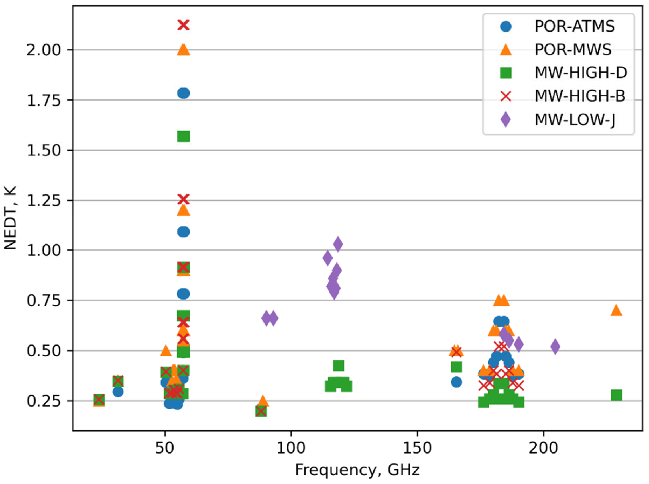
Using the two methods described in Section 2, instrument temperature and moisture retrieval vertical resolutions were computed, and retrieval error was assessed. Instrument noise prescribed for each sensor and used in those analyses are shown in Figure 1. It is clear from the figure that the MW-HIGH-D sensor spectral coverage is more complete as compared to other sensors, and the expected NEDT of the instrument is smaller than others for most bands.

In the analyses that follow, instrument noise, Se was assumed to be uncorrelated, with magnitudes shown in Figure 1. An additional 0.2K was added to the diagonal of S to account for uncertainties such as those from CRTM forward model parameterizations, spectroscopy, and calibration. Equation (1) also requires an assumption about the background variability of the atmosphere, in $S_a^{-1}$. For our computations, we utilized empirically derived errors from real MIIDAPS-AI temperature and moisture profile and surface temperature soundings from ATMS [14], scaled those by 2.0 and added an 80% ad-hoc vertical correlation between adjacent levels for both temperature and moisture.

3.2. Results for MW Instruments

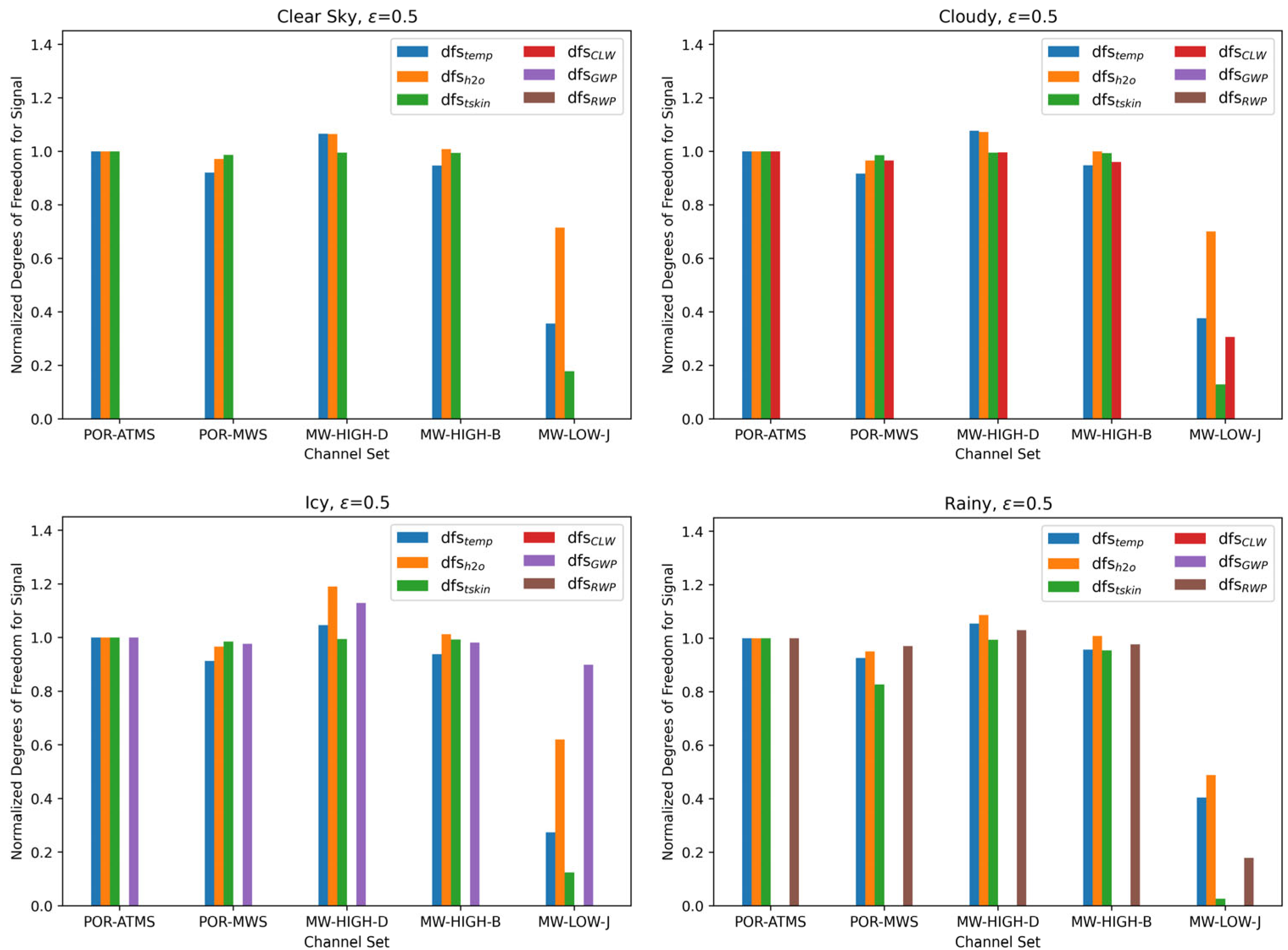
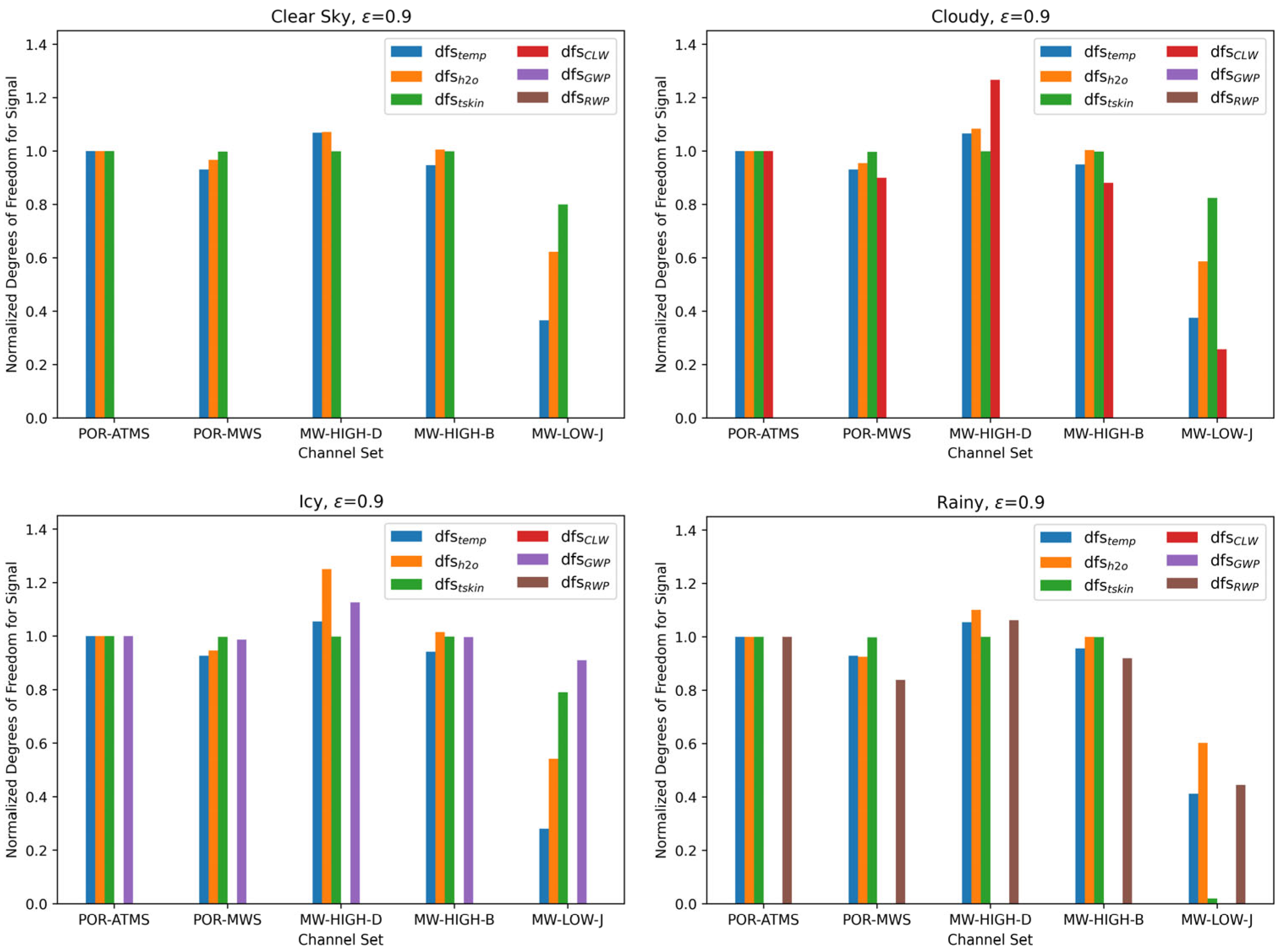
Figure 2, Figure 3 and Figure 4 show the information content and retrieval errors for five simulated MW sensor configurations, respectively. Temperature, water, surface temperature, cloud, and precipitation degrees of freedom for signal ($dfs$) were computed using Equation (1), for two emissivity (high and low to represent land-like and ocean-like conditions) and four atmospheric conditions with respect to cloud and precipitation are shown in Figure 2 and Figure 3. For each of the two emissivities assessed and each atmospheric condition, the average $dfs$ were computed for each variable over the three standard atmospheric profile simulations. The degrees of freedom for all sensors and parameters were then normalized with respect to the program of record ATMS (POR-ATMS) values.

The five sensors assessed include POR-ATMS, a program of record MWS (a European follow-on sensor to AMSU), MW-HIGH-B/D (lower noise and digital ATMS), as well as the MW-LOW-J (TROPICS-like) sensor. In general, the digital ATMS sensor (MW-HIGH-D) outperforms all other sensors for all parameters with increased $dfs,$ sometimes increasing more than 15%. MW-HIGH-B, POR-MWS, and POR-ATMS show similar performance (within 10%) with respect to vertical resolution. The differences between those four sensors is largely due to instrument noise, i.e., noise is a significant driver of MW vertical resolution, especially at 50 GHz. MW-LOW-J is the worst performing sensor, showing a normalized $dfs$ of 50% or smaller for temperature and moisture as compared to all other sensor configurations. The reduction in instrument performance is largely due to increased noise at the 118 GHz temperature sounding bands, however at 118 GHz the single O₂ line vertical weighting functions for temperature are broader than similar channels in the 50 GHz portion of the MW spectrum [20]. Higher frequency (118 GHz and 220 GHz) bands on MW-LOW-J are also radiatively more sensitive to the spectral signature of ice which explains the reduced temperature and moisture $dfs$ in icy conditions as compared to other sensors.

Cloud and precipitation retrieval information content were also assessed for the four model atmospheres. Normalized values are shown in Figure 2 and Figure 3, however most sensor configurations are sensitive to 0.5–1 $dfs$ (integrated column) for cloud liquid water. Precipitating graupel/snow and rain $dfs$ are between 1 and 2 $dfs$ indicating some sensors have some profile-sensing capability albeit limited to a vertical shift in the profile. As expected, graupel sensitivity is somewhat enhanced over higher emissivity (land-like) while rain sensitivity is somewhat enhanced over lower emissivity surfaces (ocean-like).

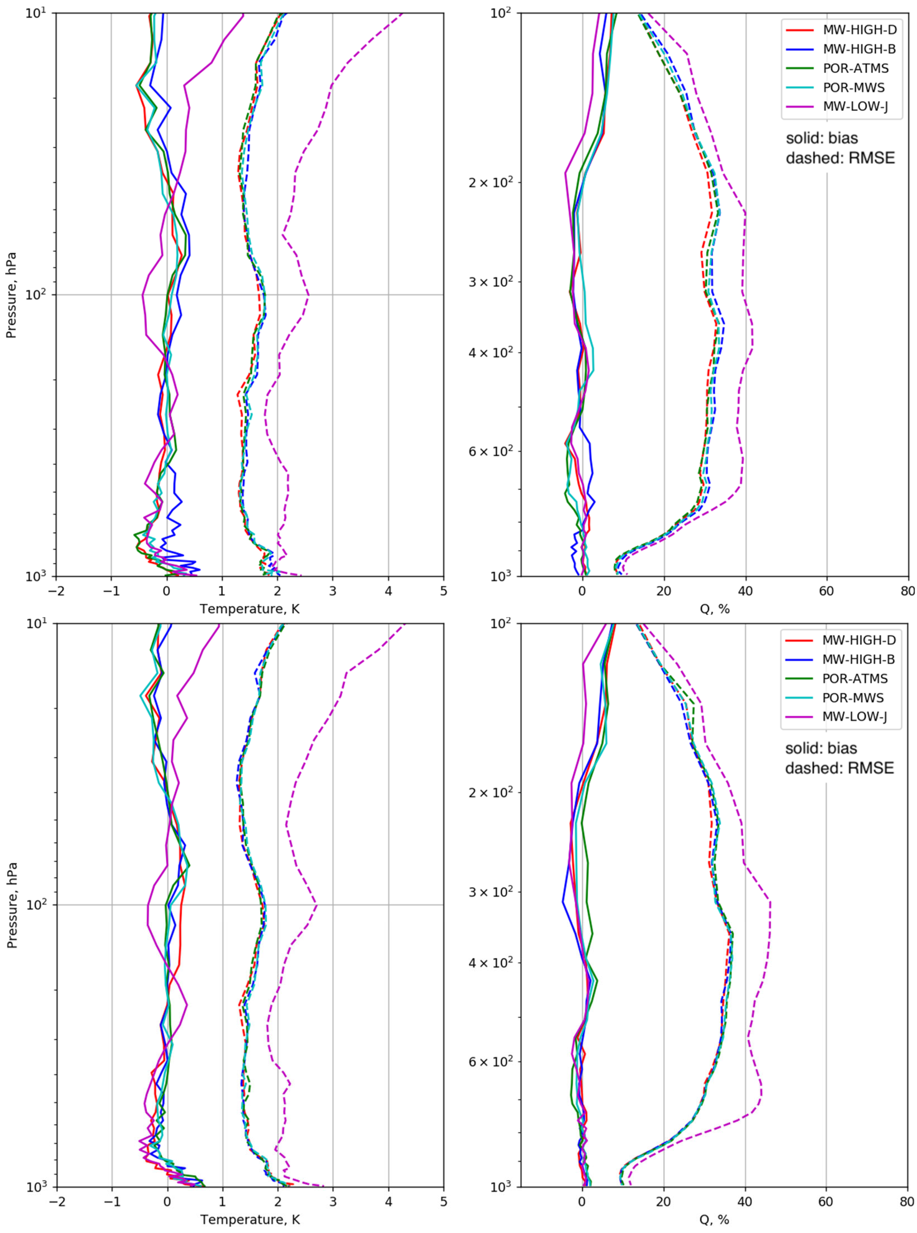
The assessment shown in Figure 4 illustrates that while the vertical resolution computed shows significant deviations for the program of record instruments and MW-HIGH-B/D sensors, the actual performance from a remote sensing algorithm is much more nuanced. In general, the mean biases of MIIDAPS-AI minus G5NR for temperature and moisture are small (less than 0.5K for temperature and a few percent for specific humidity). This is somewhat expected given that the assessment is performed using simulated satellite observations without systematic calibration or forward model errors. Comparing MW-HIGH-D (best performing sensor) to MW-HIGH-B and POR-ATMS/MWS for clear-sky condition, we can conclude that the 10–20% differences in the sensor vertical resolution, represented in the $dfs$, translate to a maximum 0.1K temperature retrieval RMSE and 2–5% water vapor RMSE (see Figure 4). It is difficult to see any differences in these sensors in the all-sky comparisons, indicating that when averaged over a day and over the globe, the information content controlling factors in clear-sky are less important in cloudy and precipitating conditions. Nevertheless, in icy conditions, Figure 3 and Figure 4 show significantly increased water vapor $dfs$ for the MW-HIGH-D compared to other sensors. Offline simulation experiments (not shown) of a MW-HIGH-D sensor with and without higher frequencies suggest that the combination of 50 GHz/118 GHz on the MW-HIGH-D sensor offer unique information which enable the separation of water and ice/graupel spectral signatures and therefore improve the sounding of water in icy conditions.

The impact of the 50% reduction in temperature and moisture $dfs$ for the MW-LOW-J sensor is more apparent in Figure 4. Compared to other sensors assessed, MIIDAPS-AI temperature standard deviations versus G5NR for the MW-LOW-J sensor are 0.5K larger in the troposphere and up to 2K larger in the stratosphere due to the lack of more absorptive channels at 118 GHz. The water statistical assessments show a similar trend in the troposphere with a 10% increased water RMSE in the clear-sky conditions and 15% in all-sky conditions as compared to the other sensors assessed. The reduced number of moisture profiling sounding channels and increased sensitivity to ice at higher frequencies likely explains that behavior.

4. Discussion

The objective of this study was to provide a consistent theoretical and empirical (for MW) assessment of the major driving factors of the information content ($dfs$) for current and potential future MW instruments. The theoretical assessments used well-defined information content analysis based on CRTM simulations, expected instrument and forward model noise, and atmospheric variability based on real geophysical retrievals from MIIDAPS-AI. These assessments were computed for multiple atmospheric conditions at nadir; however, similar conclusions were drawn for other angles (not shown). Empirical considerations used the next generation AI-based 1 dimensional-variational (1DVAR) emulator MIIDAPS-AI applied to global and multi-seasonal noise-added simulations from NASA’s G5NR in clear and cloudy/precipitating conditions.

Our analyses for the MW sounding instruments assessed showed that instrument noise is a major driver of information content, especially at 50 GHz. Nevertheless, empirical assessments of instruments with 50 GHz bands found 10–20% differences in the sensor vertical resolution translated to a maximum 0.1K temperature retrieval RMSE and 2–5% water vapor RMSE; especially in clear-sky conditions. Our assessment was performed using pre-defined sensor bandwidths and channel centers, and most of the sensors we assessed possessed similar sensor characteristics with respect to channel frequencies. Optimization of the selection of the number bands and their bandwidths across the microwave spectrum would be the most significant driver of the information content and performance of sensors possessing 50 GHz sounding channels [20].

Our assessment of a TROPICS-like sensor which utilizes the 118 GHz O₂ line for temperature sounding found a significant degradation in both assessments; especially in icy precipitating atmospheres. These are due to higher noise, wider kernel functions in that sounding band [21], and potentially the higher sensitivity to ice at higher frequencies. Future work should therefore assess sensor performances separately in clear-sky and the different all-sky conditions, i.e., separate empirical assessments for icy-only, rainy-only, and cloudy-only conditions.

While crucially important for many regional and global applications, our analyses do not fully address how sounding density and spatial resolution, cost, temporal refresh, stability/calibration, radiative transfer uncertainties (spectroscopy and cloudy/precipitation parameterizations) affect the benefit (cost/value) of hypothetical instruments and constellations of sensors in the global observing system. Assessment of the value of new sensor or sensor constellations in the global observing system should account not only for the information content of single sensors, but also, their expected benefit to the entire suite of satellite sensors currently flying as well as ground and in situ observations. Authors should discuss the results and how they can be interpreted from the perspective of previous studies and of the working hypotheses. The findings and their implications should be discussed in the broadest context possible. Future research directions may also be highlighted.

References

- Boukabara, S.A.; Garrett, K.; Kumar, V.K. Potential Gaps in the Satellite Observing System Coverage: Assessment of Impact on NOAA’s Numerical Weather Prediction Overall Skills. Mon. Weather. Rev. 2016, 144, 2547–2563. [Google Scholar] [CrossRef]
- Menzel, W.P.; Schmit, T.J.; Zhang, P.; Li, J. Satellite-Based Atmospheric Infrared Sounder Development and Applications. Bull. Am. Meteorol. Soc. 2018, 99, 583–603. [Google Scholar] [CrossRef]
- Li, Z.; Li, J.; Schmit, T.J.; Wang, P.; Lim, A.; Li, J.; Nagle, F.W.; Bai, W.; Otkin, J.A.; Atlas, R.; et al. The alternative of CubeSat-based advanced infrared and microwave sounders for high impact weather forecasting. Atmosp. Ocean. Sci. Lett. 2019, 12, 80–90. [Google Scholar] [CrossRef]
- Pagano, T.S.; Abesamis, C.; Andrade, A.; Aumann, H.; Gunapala, S.; Heneghan, C.; Jarnot, R.; Johnson, D.; Lamborn, A.; Maruyama, Y.; et al. Design and development of the CubeSat Infrared Atmospheric Sounder (CIRAS). In Earth Observing Systems XXII.; Butler, J.J., Xiong, X.J., Gu, X., Eds.; International Society for Optics and Photonics SPIE: Bellingham, WA, USA, 2017; Volume 10402, pp. 85–92. [Google Scholar] [CrossRef]
- Blackwell, W.; Braun, S.A.; Bennartz, R.; Velden, C.S.; DeMaria, M.; Atlas, R.; Dunion, J.P.; Marks, F.D., Jr.; Rogers, R.; Annane, B. The NASA TROPICS Cubesat Constellation Observatory. In Proceedings of the First Conference on Earth Observing SmallSats and the 22nd Conference on Satellite Meteorology and Oceanography, Virtual, 20–24 September 2021; Earth Observing SmallSats: The New Normal. AMS: Austin, TX, USA, 2018. Available online: https://ams.confex.com/ams/98Annual/webprogram/Paper332554.html (accessed on 20 March 2022).
- Shahroudi, N.; Zhou, Y.; Boukabara, S.-A.; Ide, K.; Zhu, T.; Hoffman, R. Global analysis and forecast impact assessment of CubeSat MicroMAS-2 on numerical weather prediction. J. Appl. Remote Sens. 2019, 13, 032511. [Google Scholar] [CrossRef]
- Ali, A.D.S.; Rosenkranz, P.W.; Staelin, D.H. Atmospheric Sounding Near 118 GHz. J. Appl. Meteorol. 1980, 19, 1234–1238. [Google Scholar] [CrossRef] [Green Version]
- Birman, C.; Mahfouf, J.-F.; Milz, M.; Mendrok, J.; Buehler, S.A.; Brath, M. Information content on hydrometeors from millimeter and sub-millimeter wavelengths. Tellus A Dyn. Meteorol. Oceanogr. 2017, 69, 1271562. [Google Scholar] [CrossRef]
- McCarty, W.; National Aeronautics and Space Administration. Personal communication, 2020.
- Chevallier, F.; Bauer, P.; Mahfouf, J.-F.; Morcrette, J.-J. Variational retrieval of cloud profile from ATOVS observations. QJR Meteorol. Soc. 2002, 128, 2511–2525. [Google Scholar] [CrossRef]
- Bauer, P.; Moreau, E.; Chevallier, F.; O’Keeffe, U. Multiple-Scattering Microwave Radiative Transfer for Data Assimilation Applications; Technical Report 486; ECMWF: Reading, UK, 2006; Available online: https://www.ecmwf.int/node/7989 (accessed on 5 October 2021).
- Ding, S.; Yang, P.; Weng, F.; Liu, Q.; Han, Y.; van Delst, P.; Li, J.; Baum, B. Validation of the community radiative transfer model. J. Quant. Spectrosc. Radiat. Transf. 2011, 112, 1050–1064. [Google Scholar] [CrossRef]
- Rodgers, C.D. Inverse Methods for Atmospheric Sounding: Theory and Practice; World Scientific: Singapore; Hackensack, NJ, USA, 2000. [Google Scholar] [CrossRef]
- Maddy, E.S.; Boukabara, S.-A. MIIDAPS-AI: An Explainable Machine-Learning Algorithm for Infrared and Microwave Remote Sensing and Data Assimilation Preprocessing—Application to LEO and GEO Sensors. IEEE J. Sel. Top. Appl. Earth Obs. Remote Sens. 2021, 14, 8566–8576. [Google Scholar] [CrossRef]
- Gelaro, R.; Putman, W.M.; Pawson, S.; Draper, C.; Molod, A.; Norris, P.M.; Ott, L.; Privé, N.; Reale, O.; Achuthavarier, D.; et al. 2015: Evaluation of the 7-km GEOS-5 Nature Run; NASA Technical Memorandum. NASA/TM-2014-104606; Koster, R.D., Ed.; Technical Report Series on Global Modeling and Data Assimilation; National Aeronautics and Space Administration: Greenbelt, MD, USA, 2015; Volume 36, 285p. Available online: http://gmao.gsfc.nasa.gov/pubs/docs/Gelaro736.pdf (accessed on 1 February 2022).
- Boukabara, S.-A.; Moradi, I.; Atlas, R.; Casey, S.P.F.; Cucurull, L.; Hoffman, R.N.; Ide, K.; Kumar, V.K.; Li, R.; Li, Z.; et al. Community Global Observing System Simulation Experiment (OSSE) Package (CGOP): Description and Usage. J. Atmos. Ocean. Technol. 2016, 33, 1759–1777. [Google Scholar] [CrossRef]
- Boukabara, S.; Ide, K.; Shahroudi, N.; Zhou, Y.; Zhu, T.; Li, R.; Cucurull, L.; Atlas, R.; Casey SP, F.; Hoffman, R.N. Community Global Observing System Simulation Experiment (OSSE) Package (CGOP): Perfect Observations Simulation Validation. J. Atmos. Ocean. Technol. 2018, 35, 207–226. [Google Scholar] [CrossRef]
- Mattioli, V.; Accadia, C.; Ackermann, J.; Di Michele, S.; Hans, I.; Schlüssel, P.; Colucci, P.; Canestri, A. The EUMETSAT polar systems Second generation (EPS-SG) passive microwave and Sub-mm wave missions. In Proceedings of the 41st PhotonIcs & Electromagnetics Research Symposium—Spring (PIERS-Spring), Rome, Italy, 17–20 June 2019; pp. 3926–3933. [Google Scholar]
- Blackwell, W.; Allen, G.; Galbraith, C.; Hancock, T.; Leslie, R.; Osaretin, I.; Retherford, L.; Scarito, M.; Semisch, C.; Shields, M.; et al. Nanosatellites for earth environmental monitoring: The micromas project. In Proceedings of the 2012 12th Specialist Meeting on Microwave Radiometry and Remote Sensing of the Environment (MicroRad), Rome, Italy, 5–9 March 2012; pp. 1–4. [Google Scholar]
- Kummerow, C.D.; Poczatek, J.C.; Almond, S.; Berg, W.; Jarrett, O.; Jones, A.; Kantner, M.; Kuo, C.-P. Hyperspectral Microwave Sensors—Advantages and Limitations. IEEE J. Sel. Top. Appl. Earth Obs. Remote Sens. 2022, 15, 764–775. [Google Scholar] [CrossRef]
- Prigent, C.; Pardo, J.R.; Rossow, W.B. Comparisons of the Millimeter and Submillimeter Bands for Atmospheric Temperature and Water Vapor Soundings for Clear and Cloudy Skies. J. Appl. Meteorol. Clim. 2006, 45, 1622–1633. [Google Scholar] [CrossRef] [Green Version]