Optical Design of a Common-Aperture Camera for Infrared Guided Polarization Imaging

Abstract

Polarization and infrared imaging technology have unique advantages for various applications ranging from biology to ocean remote sensing. However, conventional combined polarization camera and infrared camera have limitations because they are constrained to single-band imaging systems with rotating polarizers and cascaded optics. Therefore, we propose a common-aperture mode based on multi-band infrared guided polarization imaging system (IGPIS) in this paper, which consists of infrared wide-area sensing and polarization features acquisition for accurate detection of ship targets. The IGPIS can provide images in visible polarization (0.45–0.76 μm), near-infrared polarization (0.76–0.9 μm), and long-wave infrared (8–12 μm) bands. Satellite attitude parameters and camera optical parameters are accurately calculated by establishing a dynamic imaging model for guidance imaging. We illustrate the imaging principle, sensors specifications and imaging performance analysis and the experimental results show that the MTF is 0.24 for visible and near-infrared, and 0.13 for long-wave infrared. The obtained multi-band images have an average gradient of 12.77 after accurate fusion. These results provide theoretical guidance for the design of common-aperture cameras in remote sensing imaging field.

1. Introduction

Remote sensing technology can quickly provide image data in many accidental ocean disasters such as floods, tsunami rescues, sea ice and territorial invasions [1,2,3,4]. In recent years, infrared imaging can work around the clock and has a good ability to penetrate clouds, which plays a crucial role in ocean remote sensing. However, due to the development of infrared camouflage coating and infrared stealth technologies, as well as the interference of decoys and sea clutter, the contrast between the targets and the background radiation is greatly reduced, which is called isomeric colors. This makes infrared images with low resolution that lack details and texture features, which severely limit the detection effect. The radiation intensity characteristic of infrared imaging is only a branch of the polarized radiation characteristic. Polarization imaging systems provide valuable information about the imaging environment, such as the shape, texture, scattering degree, and metallicity of reflective surfaces. Touzi utilized polarimetric data to verify the application of symmetric phase for wetland classification, in particular [5]. Muhuri et al., analyzed the polarization indicators and tracked their time in satellite imaging, so as to detect target [6]. On the basis of the above, it can be seen that polarization imaging captures particular optical information about imaged environments, which is usually absent in intensity and spectral content. As ocean observations need better spatial resolution and more detailed information, polarization technology is widely used. There are two detection methods that can distinguish the isomeric colors: One is the multi-band imaging system. Topaz et al., designed a near/mid-infrared common-aperture imaging system using the Cassegrain optical system, which was mainly used for large-scale target detection [7]. Levan designed a mid/long-wave infrared common-aperture imaging spectrometer that utilized the beam splitting properties of a flat mirror to obtain spectral images in two fields of view (FOV) [8]. Hiroshi developed an airborne multi-spectral polarization imager, which used four cameras with multi-polarization (MP) and filter wheels to achieve multi-degree polarization imaging [9]. The other is the single-band polarization imaging system. Huang et al., studied the theory of the infrared polarization imaging model, and carried out experiments on infrared polarization targets [10]. The US Air Force Laboratory used the long-wave infrared micro-polarization system to conduct the target tracking experiment. The results showed that the long-wave infrared polarization technology could improve the recognition ability of targets in complex backgrounds [11]. Some studies have established relevant imaging models [12,13,14,15,16,17,18,19] and these systems are limited to single-band cameras with infrared polarization measurement capability. However, there is no mature theoretical framework for multi-band imaging systems in this field. In summary, under the same interference conditions, the infrared polarization imaging system has better detection performance than the traditional infrared imaging system. Aiming at dynamic targets distributed in a wide area on the ocean, the concept of infrared-guided polarization (IGP) is introduced, which is a dual-source collaborative imaging mode that recognizes while sensing. In the IGP imaging mode, system parameters such as material characteristics of targets, the performance of multi-band payloads, satellite attitude, and orbital maneuverability, are considered to solve the problem of on-orbit restrictions. Our system presents IGP imaging mode and calculates the three-axis attitude of the satellite and optical system parameters. In this paper, we propose a common-aperture imaging system that can simultaneously capture infrared and polarization information. The system innovatively utilizes a transflective mirror covered with a high-reflective film to transmit light in the infrared system and reflect light in the polarization system. The spectrum ranges from 450 nm to 900 nm with a spatial resolution of 11.5 m @ at 500 km and 8 μm to 12 μm (long-wave infrared) with a spatial resolution of 115 m at 500 km. Compared with multifunctional satellites which consist of two optical system namely, the directional polarimetric camera and the long-wave infrared camera. Our system possesses the advantages of compactness, light weight, and low cost, although the spatial resolution of infrared system is lower. Furthermore, the outfield imaging experiment is built based on these basic principles and our optical design. According to the weight of the energy factor, dual-source fusion is performed on the target in the infrared and polarized images which are obtained by the experiment. The proposed common-aperture imaging system provides a new possibility for real-time response of ocean remote sensing.

2. Principle and Imaging Mode

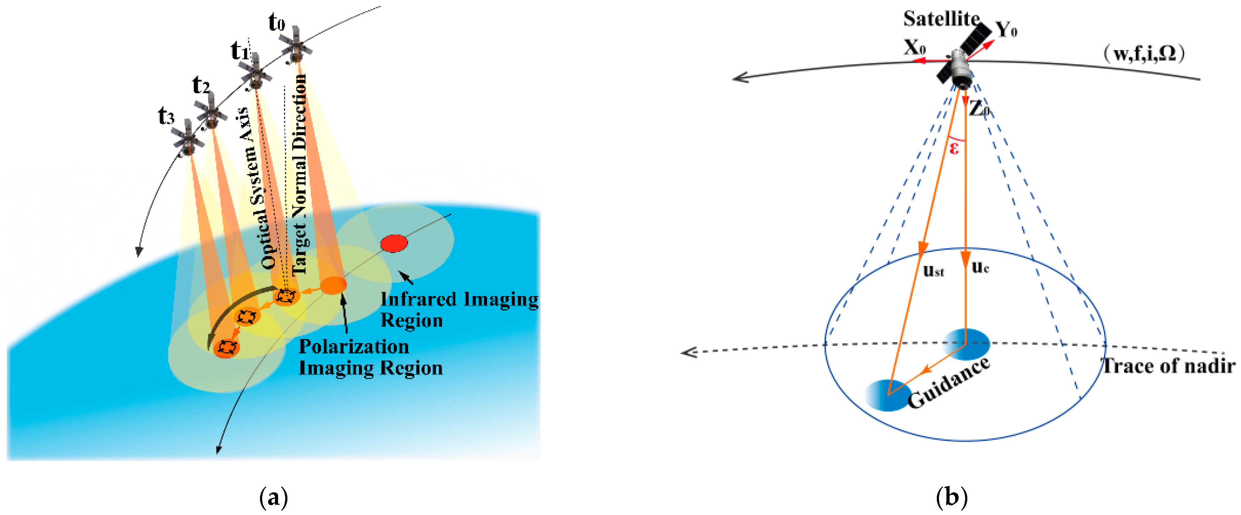
2.1. IGP Imaging Model

A multi-band IGP imaging model based on a common-aperture optical system was used, as shown in Figure 1a. Firstly, we utilize a large field of view of the infrared system to search and locate the target. Then the satellite locks onto the dynamic target to obtain the direction and controls the attitude, thus guiding the polarization system to target the image. Specifically, during the imaging search, the three-axis attitude angle of the satellite is held to achieve stable imaging. When the intended target appears, the optical axis is pointed to the target by changing the satellite’s attitude for accurate polarization imaging. In order to optimally utilize satellite resources, the satellite’s attitude angle is calculated by the quaternion which is the shortest path. The expected quaternion is calculated continuously, so that the optical axis of the camera is coincident with the target observation vector. In the on-orbit attitude control, there are many path options for the guidance. Therefore, it is necessary to optimize the path to achieve the best guidance imaging. As shown in Figure 1b, the satellite has a guidance path for maneuvering from the current attitude to the desired attitude. In the Earth’s inertial coordinate system, the position vectors of the observation satellite and the target can be expressed as $r_s(x_s,y_s,z_s)$ and $r_t(x_t,y_t,z_t)$ at the current time.

The unit observation vector of the target in the satellite orbital coordinate system can be expressed as:

$${\mathit{u}}_{\mathit{s}\mathit{t}}=\frac{M_I^O\cdot ({\mathit{r}}_t-{\mathit{r}}_{\mathit{s}})}{\Vert {\mathit{r}}_t-{\mathit{r}}_{\mathit{s}}\Vert }$$

(1)

where $\Vert {\mathit{r}}_t-{\mathit{r}}_{\mathit{s}}\Vert$ is the distance between the observation satellite and the target, which can be expressed as:

$$\Vert {\mathit{r}}_t-{\mathit{r}}_{\mathit{s}}\Vert =\sqrt{{\left(x_t-x_s\right)}^2+{\left(y_t-y_s\right)}^2+{\left(z_t-z_s\right)}^2}$$

(2)

where $M_I^O$ is the conversion matrix from the earth’s inertial coordinate system to the satellite’s orbit coordinate system, which can be expressed as:

$$M_I^O=B\cdot R_z(\omega +f)\cdot R_x(i)\cdot R_z(\Omega )$$

(3)

where $\omega$ is the argument of perigee, $f$ is the true anomaly, $i$ is the orbital inclination, $\Omega$ is the ascending node right ascension, and $R_x(\cdot ),R_z(\cdot )$ are the rotation matrices of the current coordinate system around the x- and z-axes, respectively, which are expressed as

$$R_x(\cdot )=\left(\begin{array}{ccc}1& 0& 0\\ 0& \cos (\cdot )& -\sin (\cdot )\\ 0& \sin (\cdot )& \cos (\cdot )\end{array}\right),R_z(\cdot )=\left(\begin{array}{ccc}\cos (\cdot )& -\sin (\cdot )& 0\\ \sin (\cdot )& \cos (\cdot )& 0\\ 0& 0& 1\end{array}\right).$$

$B$ is the adjust matrix for the coordinate axis, which can be expressed as $B=\left[\begin{array}{ccc}0& 1& 0\\ 0& 0& -1\\ -1& 0& 0\end{array}\right]$. At the same time, the unit vector ${\mathit{u}}_{\mathit{c}}$ of the optical axis of the camera in the orbital coordinate system can represent ${\mathit{u}}_{\mathit{c}}=(0,0,1)$. The expected quaternion is:

$${\mathit{Q}}_{\mathit{c}}=\left[\begin{array}{cc}\cos \frac{\epsilon }{2}& \mathit{e}\sin \frac{\epsilon }{2}\end{array}\right]=\left[\begin{array}{cccc}{q}_0& q_1& q_2& q_3\end{array}\right]$$

(4)

where $\epsilon$ is the angle between the observation vector and the direction of the optical axis, and $e$ is the Euler axis vector that is perpendicular to the two vectors, which is expressed as follows:

$$\{\begin{array}{l}\epsilon =\arccos ({\mathit{u}}_{\mathit{c}}\cdot {\mathit{u}}_{\mathit{s}\mathit{t}})\\ \mathit{e}={\mathit{u}}_{\mathit{c}}\times {\mathit{u}}_{\mathit{s}\mathit{t}}\end{array}$$

(5)

Since the observation satellite has no angular velocity components in the ${\mathit{u}}_{\mathit{s}\mathit{t}}$ and ${\mathit{u}}_{\mathit{c}}$ directions, the satellite’s optimal steering path is of the shortest angular distance. When the satellite rotates in an order of 3-1-2, according to the expected attitude quaternion Equation (4), the expected yaw angles $\psi$ of the satellite body coordinate system relative to the orbital coordinate system, the roll angle $\phi$ and the pitch angle $\theta$ are calculated as:

$$\{\begin{array}{l}\psi =\arctan [\frac{2(q_1{q}_2+q_3{q}_0)}{-q_1{}^2+q_2{}^2-q_3{}^2+q_0{}^2}]\\ \phi =\arcsin [2(q_0{q}_1-q_2{q}_3)]\\ \theta =\arctan [\frac{2(q_1{q}_3+q_2{q}_0)}{-q_1{}^2-q_2{}^2+q_3{}^2+q_0{}^2}]\end{array}$$

(6)

The expected three-axis rotation Euler angles, $\psi$, $\phi$, $\theta$, allow the satellite to control its attitude to achieve corresponding attitude rotation [20,21]. Real-time iterative calculation is carried out during the rotation process to realize the generation of the speed vector and stable control of attitude. By changing the attitude of the satellite to guide imaging, the optical axis can always point to the target and the IGPIS can be synchronized to take pictures according to a predetermined change in the speed vector. When the satellite has rotated the corresponding angle, the optical axis of the camera is guided to point to the target. The model of IGP allows real-time guided imaging along the orbit and overcomes limitations of traditional single-source camera recognition, in which detection of dynamic targets cannot be achieved effectively.

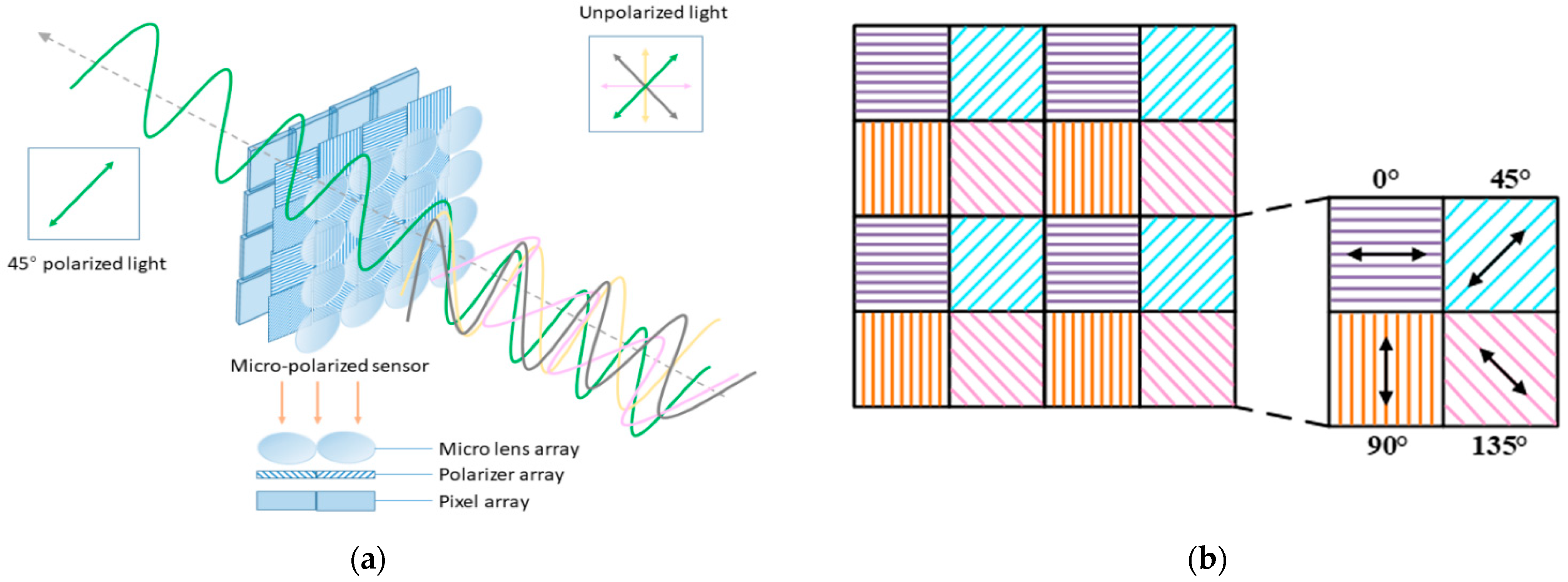
2.2. Pixel-Level Polarization Sensor

Polarization imaging devices are roughly divided into the following four categories: (1) the division of time, (2) the division of amplitude, (3) the division of aperture and (4) the division of focal plane [22,23,24]. If the division of time polarization imaging is performed on ocean targets, most of which are moving, measurement errors will be introduced. The division of amplitude is bulky and not suitable for miniaturized system. The division of aperture existed in complex optical structures and lead to difficult image registration. However, the division of focal plane polarization imaging devices can overcome these limitations as it has the advantages of good real-time performance, being a small size, and having high integration. Therefore, we choose a pixel-level polarization sensor for real-time micro-polarization imaging. Light from the sun or fluorescent lamps vibrate in various directions and are called unpolarized light. As shown in Figure 2a, when unpolarized light is transmitted through a polarizing filter, it emerges as polarized light. The sensor integrates a nanowire polarization filter, which is composed of a lens layer, a polarization information collection layer, and a photosensitive circuit layer. The polarized filter is placed directly between the pixel array and the micro lens array of the sensor. This design, compared with the polarizing filter on top of the micro lens array, reduces the possibility of light, at a polarized angle, being misdirected into an adjacent pixel (crosstalk) and incorrectly detected at the wrong angle. Micro-polarization arrays with different polarization units are the common feature of pixel polarization cameras. To explain how a pixel polarization camera records and extracts polarization information, we present Figure 2b. As shown in Figure 2b, we take $2\times 2$ micro-polarization-pixel arrays to form a super pixel unit as an example to illustrate that the array polarizer contains pixel channels for measurements. Four adjacent pixel channels form a polarization unit. The corresponding channel of each polarization unit has pixels of the nanowire polarization filter with different angles (0°, 45°, 90°, 135°). By obtaining the ratio of light from these four angles of polarization, the polarization intensity at any angle can be calculated.

3. Optical Design and Analysis

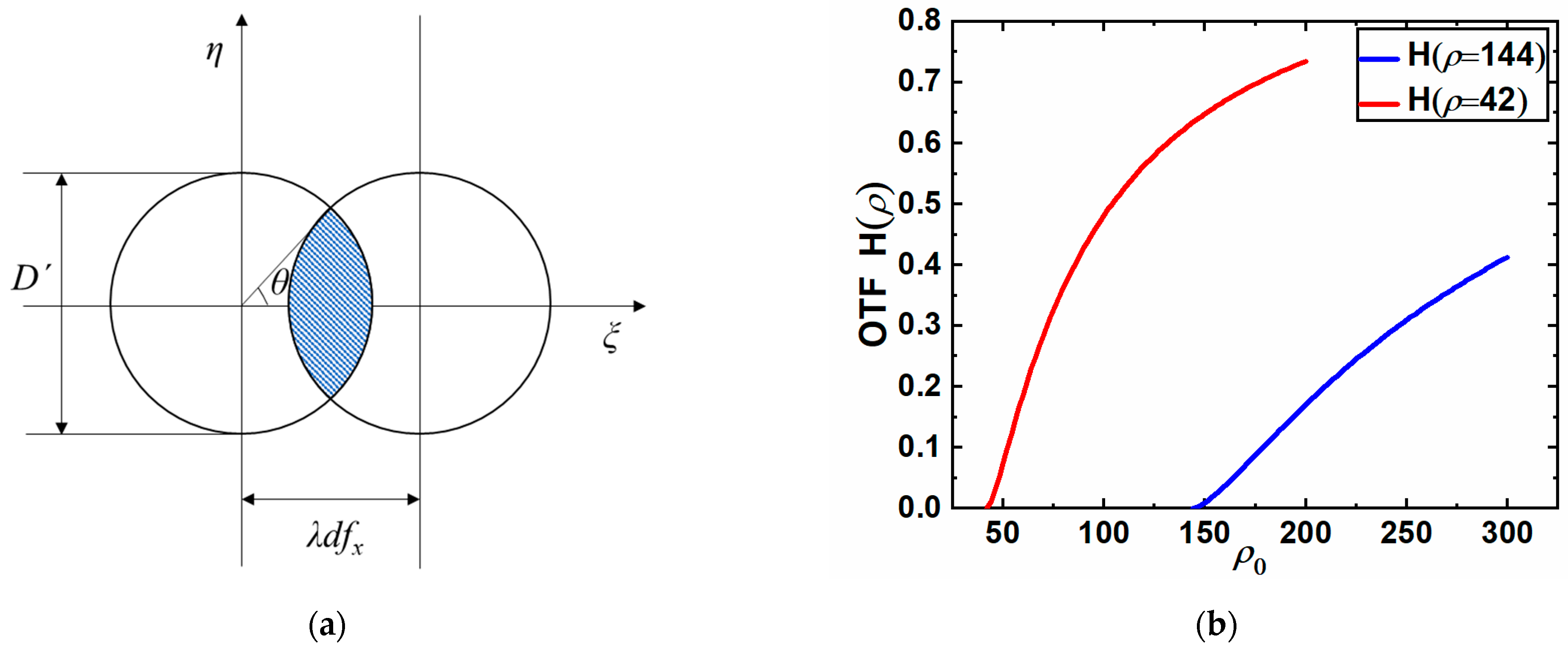
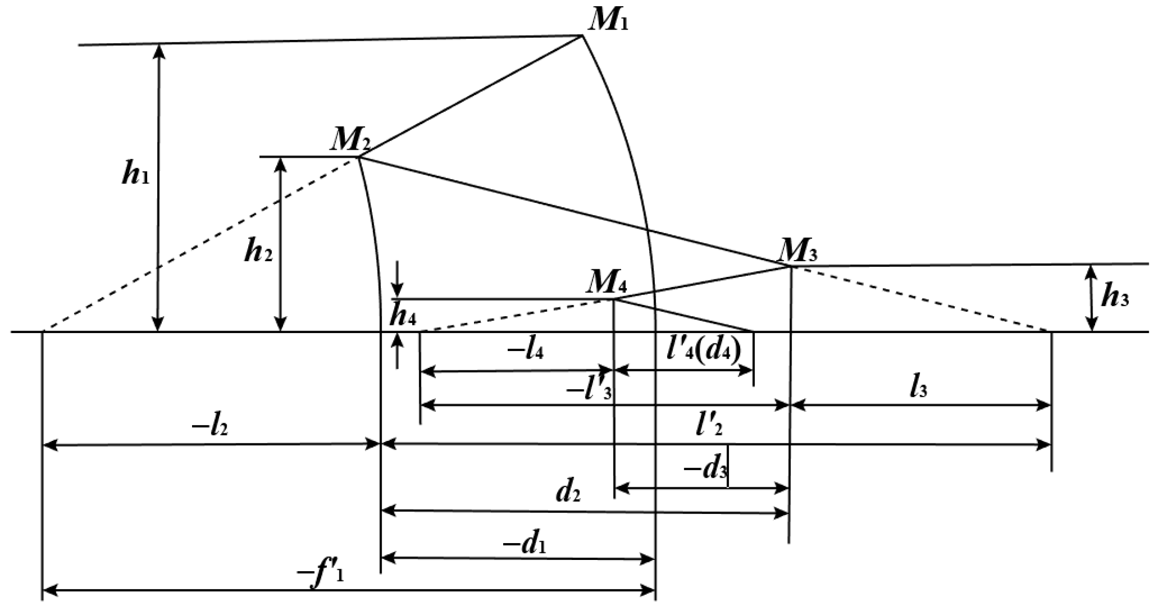
3.1. Calculation of Optical Parameter

During the imaging process of the satellite, it is necessary to ensure that the moving distance of the camera along the track is equal to the maximum coverage width. The multi-band imaging system needs to determine the camera parameters such as ground sampling distance (GSD). The scene setting of the common-aperture camera is that the GSD of the infrared imaging system is 115 m at 500 km; the pixel specification of the infrared image sensor is $p_i=14$ μm; the Polarization imaging system is 11.5 m at 500 km, the pixel specification of the infrared image sensor is $p_v=3.45$ μm; H is the height of the satellite orbit.

According to the formula $GSD/p=\mathrm{H}/f$, where $f$ is the focal length, and the calculated focal lengths of infrared imaging system and polarization imaging system are $f_i$ = 60 mm and $f_v$ = 300 mm, respectively.

According to the camera GSD index, the common-aperture parameter D needs to satisfy $D\ge \frac{1.22\lambda }{\alpha }$, where α is the angular resolution of $\alpha =\frac{p}{f}$, that is, the aperture of the infrared imaging system is $D\ge \frac{1.22{\lambda }_i{f}_i}{p_i}=52.28$ mm, and the aperture of polarization imaging system is $D\ge \frac{1.22{\lambda }_v{f}_v}{2p_v}=47.73$ mm. The above analysis process shows that the minimum value of the optimal solution of D can be obtained as 60 mm. Therefore, the calculated imaging parameters of the camera are shown in

Table 1. Imaging parameters of the camera.

Imaging Parameters	Fore-Infrared System	Rear Polarization System
Full field of view/°	8	2
Focal length/mm	60	300
GSD/m	114	11.5
Width/km	70	9

.

The IGPIS has a wide band range, and the optical system structure is complex. In the process of optimization, to accelerate the convergence speed of approaching the optimal solution, and in addition to various aberration functions, it is necessary to limit the structure function. Under the design index of camera static transfer function, the exit pupil diameter $D^{\prime }$ and exit pupil distance $d_i$ are numerically analyzed based on the scalar diffraction theory. Taking the OTF of the system as the boundary condition, we analyze the frequency characteristics of the optical imaging system. The optical transfer function (OTF) of design indexes is OTF > 0.2 at 42 lp/mm and, OTF > 0.3 at 144 lp/mm, respectively. The relationship serves as the principle to determine the initial structure of the entire system. When the system is a diffraction limited system (without considering aberrations), we can perform OTF calculations on IGPIS. The OTF of the incoherent system in the frequency domain is as follows:

$$H\left(f_x,f_y\right)=\frac{P\left(\lambda d_i{f}_x,\lambda d_i{f}_y\right)★P\left(\lambda d_i{f}_x,\lambda d_i{f}_y\right)}{{\displaystyle \int {\displaystyle {\int }_{-\infty }^{\infty }P\left(\xi ,\eta \right)d\xi d\eta }}}$$

(7)

where $P\left(\xi ,\eta \right)$ is the pupil function, the ★ is the autocorrelation symbol. The geometric interpretation of OTF can be obtained from the above formula. The diffraction limited OTF can be converted into the normalized overlap area calculation, which can be expressed as:

$$H\left(f_x,f_y\right)=\frac{S\left(f_x,f_y\right)}{S}$$

(8)

where the denominator S represents the total area of the pupil, the numerator $S\left(f_x,f_y\right)$ represents the overlapping area between the moved pupil and the original exit pupil. The central coordinate of the moved pupil is $\left(-\lambda d_i{f}_x,-\lambda d_i{f}_y\right)$. The exit pupil function is a circular symmetry function, the overlap area between the moved pupil and the original pupil is shown as the shadow area in the Figure 3a. The exit pupil function of the diffraction limited system is the circ which is obtained as follows in Equation (9). Where the unit of $\theta$ is rad, $\cos \theta =\lambda d_i{f}_x/l$.

$$H\left(f_x,0\right)=\frac{S\left(f_x,0\right)}{S}=\frac{2}{\pi }\left(\theta -\sin \theta \cos \theta \right)$$

(9)

For the radial coordinate $\rho$ in any direction of the frequency plane, there is

$$H\left(\rho \right)=\{\begin{array}{l}\frac{2}{\pi }\left[\arccos \left(\frac{\rho }{{\rho }_0}\right)-\frac{\rho }{{\rho }_0}\sqrt{1-{\left(\frac{\rho }{{\rho }_0}\right)}^2}\right],\rho \le {\rho }_0\\ 0,others\end{array}$$

(10)

where ${\rho }_0=D^{\prime }/\lambda d_i$ represents the diffraction limited. The OTF design index of the polarization branch is OTF > 0.3 @ 144 lp/mm, that is $H\left(\rho =144\right)>0.3$. The blue line represents the relation curve between ${\rho }_0$ and $H\left(\rho =144\right)$ as shown in Figure 3b. If we want $H\left(\rho =144\right)>0.3$, the condition of ${\rho }_0>246$ should be satisfied. By substituting the wavelength into the central wavelength $\lambda =0.675$ μm, the relationship between the exit pupil diameter and the exit pupil distance is $D^{\prime }/d_i>0.167$. According to the above analysis, the OTF of the infrared branch is $H\left(\rho =42\right)>0.2$, ${\rho }_0>62$ should be met as the red line as shown in Figure 3b. Substituting the wavelength into the center wavelength $\lambda =10$ μm, the relationship between the exit pupil diameter and the exit pupil distance is obtained as $D^{\prime }/d_i>0.62$.

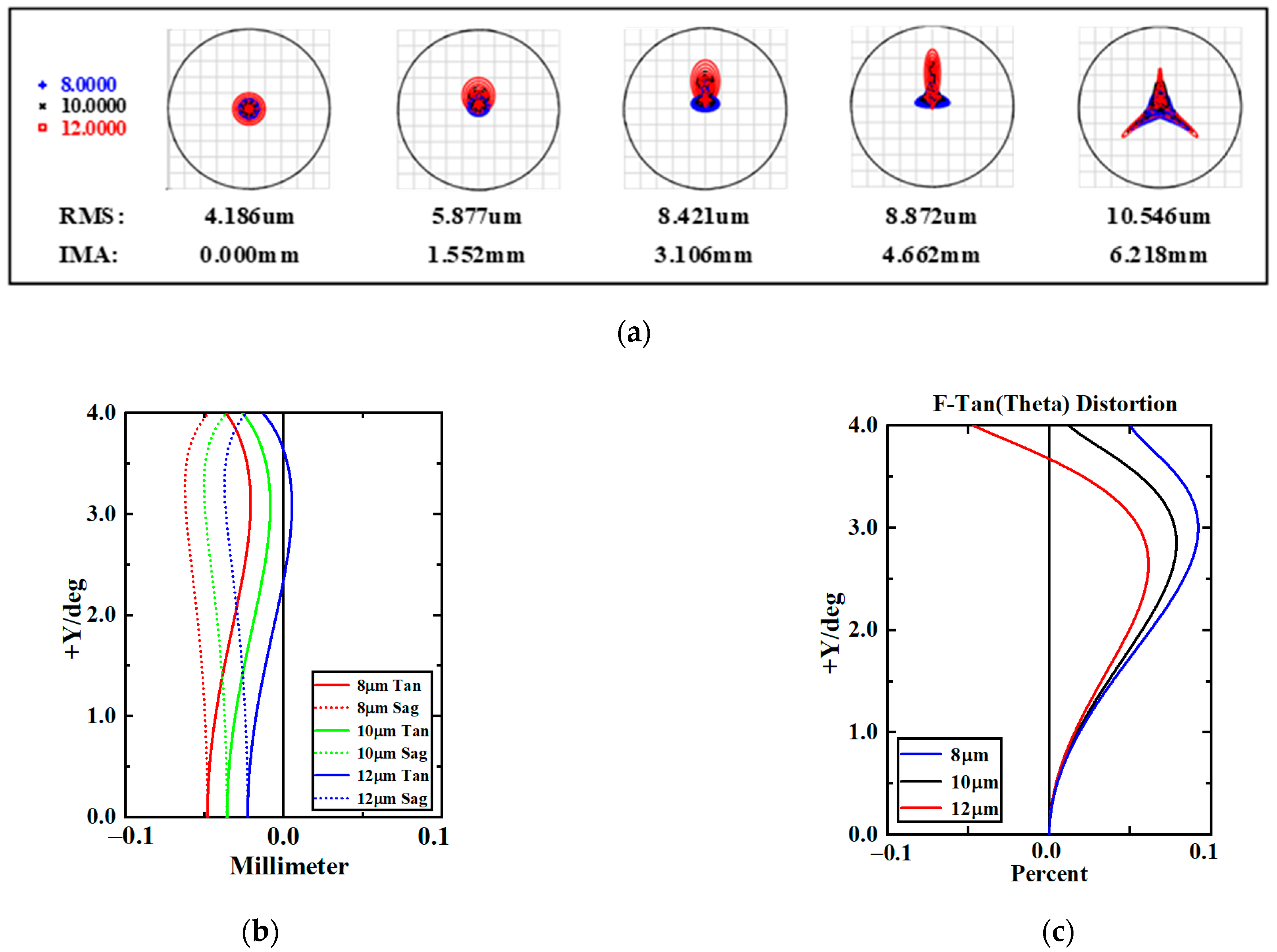
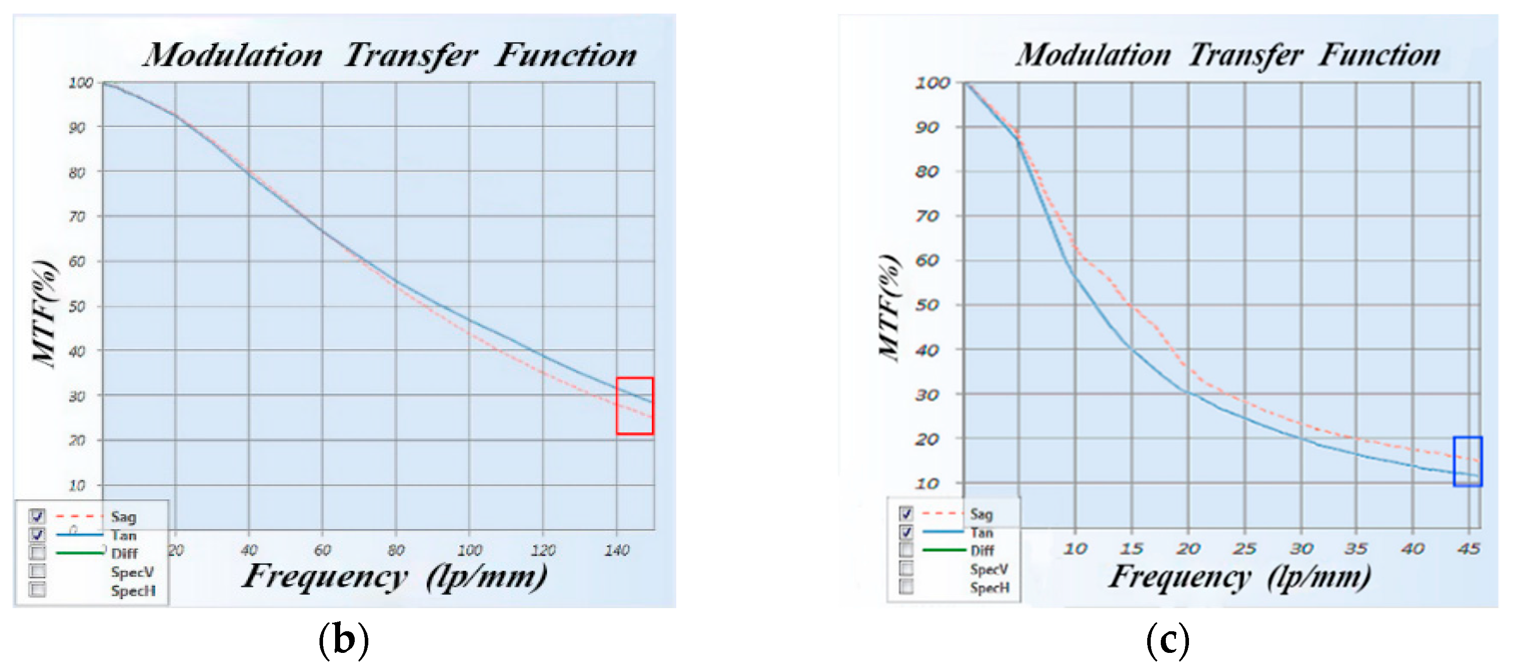
3.2. Fore-Infrared System

The fore-infrared system adopts a catadioptric scheme layout, which uses a combination of the primary mirror and the lens group. This design of the infrared imaging branch cleverly utilizes the characteristics of the large aperture and small focal length of the primary mirror. The light is not reflected by the secondary mirror, but directly enters the long-wave infrared light path after being condensed by the primary mirror, which greatly improves the relative aperture of the infrared system. The system is used for collecting the scene information from the long-wave infrared image and it is necessary to take into account the achromatic of the system. The primary mirror will not cause chromatic aberration. At the same time, the lens group can correct the aberration and enlarge the field of view of the whole optical system. In the optimal design, three types of glasses (GE_LONE, KRSS, and CLEARTRAN) are combined to achieve eliminate partial dispersion and minimize residual chromatic aberrations based on Equations (11) and (12):

$${\displaystyle \sum _{i=1}^n{h}_i^2}({\phi }_i/{\nu }_i)=0$$

(11)

$$\phi =n/f^{\prime }={\displaystyle \sum _{i=1}^n{\phi }_i}$$

(12)

where $h_i$ is the ray height of the i-th lens, ${\phi }_i$ and ${\nu }_i$ are the power and dispersion coefficient of the i-th lens respectively.

Table 2. Initial parameters of the fore-infrared system.

Surface	Radius/mm	Thickness/mm	Conic
Primary mirror	−160.45	67.23	−0.99
1st lens	−28.92	2.21	−1.66
2nd lens	−214.73	5.76	0
3rd lens	18.87	3.90	0
4th lens	−122.87	4.59	0
5th lens	−4.28	3.09	0

shows the initial parameters of the primary mirror and the lens group.

As shown in Figure 4a, the system increases the number of lenses, which is beneficial to multi-degree-of-freedom optimization design. By reducing the absorption of incident radiation, the total thickness of each lens is controlled to maximize the transmission of the long-wavelength infrared band. According to the analysis in Section 3.1, if you want the OTF of the fore-infrared system to converge quickly, set the exit pupil diameter to 16mm based on the sensor size, and set the exit pupil distance to <25.8 mm. In order to obtain the optimal system, we set the range of the exit pupil distance to [15 mm, 25 mm], and the final exit pupil distance is 23.8 mm, as is shown in Figure 4b. It can be seen that modulation transfer function (MTF), at a full field of view, exceeds 0.2 at the Nyquist frequency 42 lp/mm, approaching the diffraction limit.

Figure 5a shows the spot diagram of the whole semi-FOV of the system, from which we can see that the maximum root mean square (RMS) radius is less than one single pixel (12 µm) over the full FOV. As shown in Figure 5b, the maximum field curvature is 0.06 mm, which effectively eliminates field curvature. As shown in Figure 5c, the maximum amount of distortion is less than 0.1%. Overall, all aberrations of the fore-infrared system were corrected.

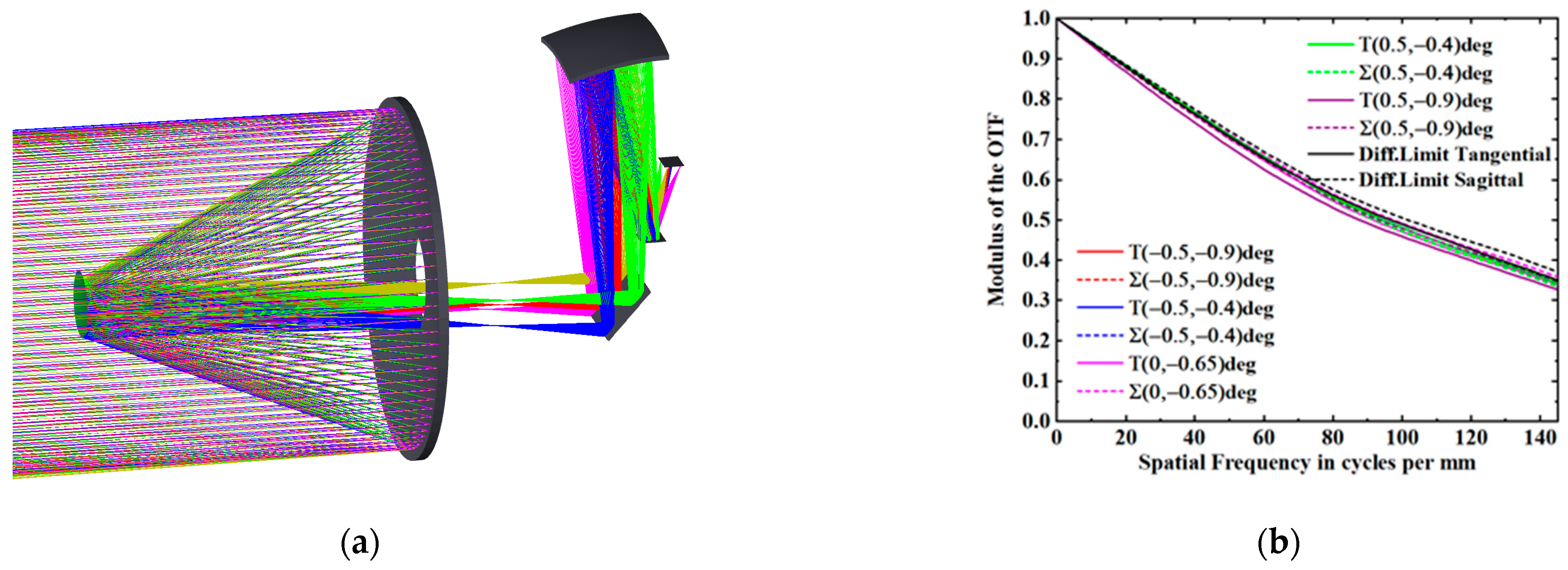
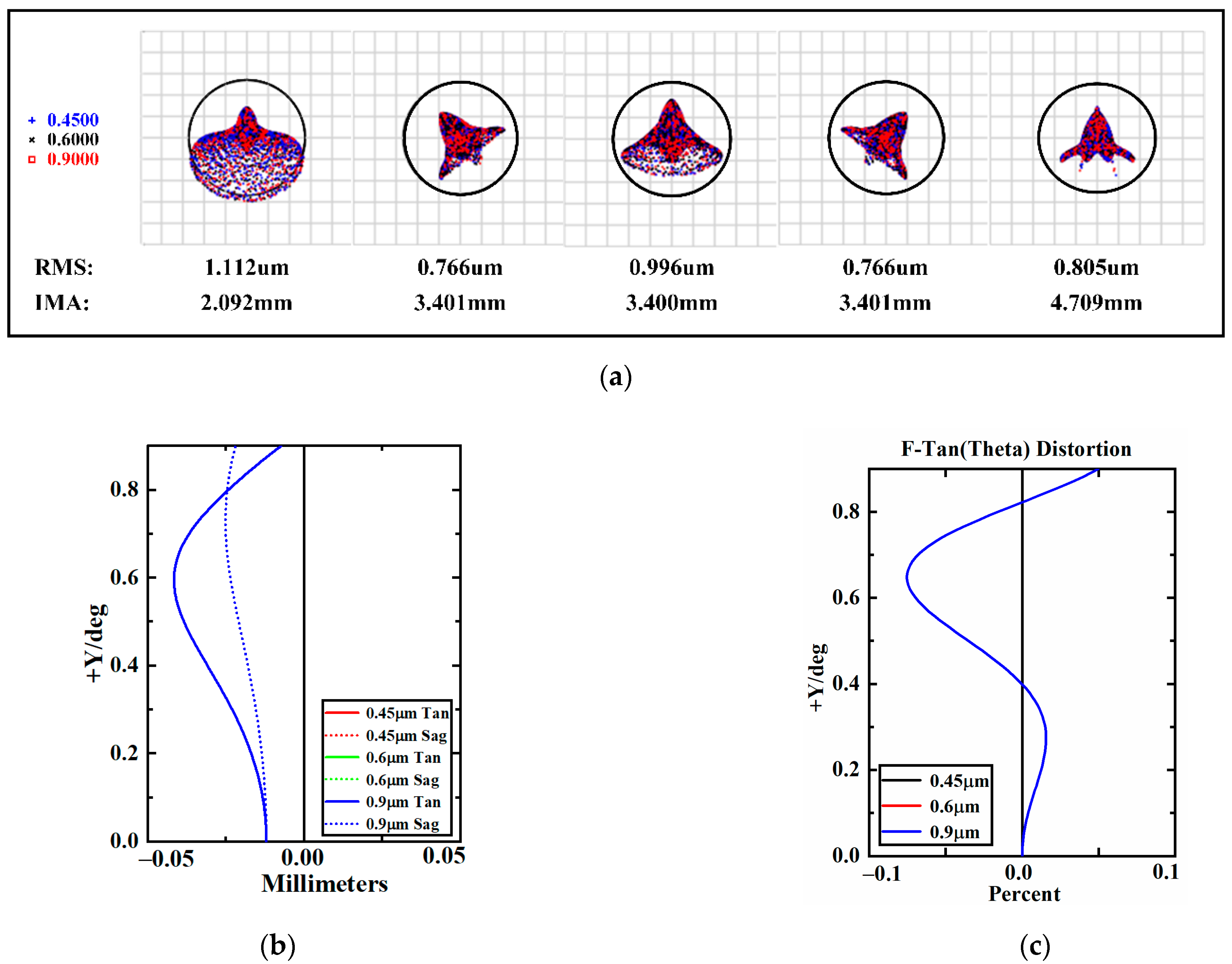
3.3. Rear-Polarization System

When the pixel-level polarization sensor and the fore-infrared system are determined, the rear-polarization system adopts a coaxial four-reflection optical scheme layout. On the principle of paraxial ray tracing basis, the relationship between the aberration coefficient and the optical parameters is established. Figure 6 is the schematic diagram of the initial structure of the four-reflection optical system [25,26,27,28].

Suppose the object is infinite, that is $l_1=-\infty$, $u_1=0$; the diaphragm is located on the primary mirror, that is $y_1=0$; for the reflective system, the radius is, $r_1,r_2,r_3,r_4$, $d_1$, $d_2$ and $d_3$ are the distances between the primary and the tertiary mirror, and the distance between the tertiary mirror and the fourth mirror respectively. $l_4^{\prime }$ is the back intercept, there is, $f^{\prime }$ is the focal length. Through the obstruction ratio ${\alpha }_1$, ${\alpha }_2$, ${\alpha }_3$, the magnification ratio ${\beta }_1$, ${\beta }_2$, ${\beta }_3$, the surface parameters of the system and the distance between the mirrors can be calculated by Equations (13) and (14):

$$\{\begin{array}{l}{r}_1=\frac{2}{{\beta }_1{\beta }_2{\beta }_3}{f}^{\prime },r_1=\frac{2{\alpha }_1}{(1+{\beta }_1){\beta }_2{\beta }_3}{f}^{\prime }\\ r_3=\frac{2{\alpha }_1{\alpha }_2}{(1+{\beta }_2){\beta }_3}{f}^{\prime },r_4=\frac{2{\alpha }_1{\alpha }_2{\alpha }_3}{1+{\beta }_3}{f}^{\prime }\end{array}$$

(13)

$$\{\begin{array}{l}{d}_1=\frac{1-{\alpha }_1}{{\beta }_1{\beta }_2{\beta }_3}{f}^{\prime },d_1=\frac{{\alpha }_1(1-{\alpha }_1)}{{\beta }_2{\beta }_3}{f}^{\prime }\\ d_3=\frac{{\alpha }_1{\alpha }_2(1-{\alpha }_3)}{{\beta }_3}{f}^{\prime },l_4^{\prime }={\alpha }_1{\alpha }_2{\alpha }_3{f}^{\prime }\end{array}$$

(14)

The above solution is brought into the third-order aberration formula to calculate and eliminate the aberration. The initial parameters are shown in

Table 3. Initial parameters of the rear polarization system.

Surface	Radius/mm	Thickness/mm	Conic
Primary mirror	−160.45	67.23	−0.99
Secondary mirror	−28.92	104.16	−1.66
Tertiary mirror	65.41	35.00	−1.48
fourth mirror	−80.25	16.38	1.24

. On this basis, tertiary mirrors and fourth mirrors are off-axis deviated from the pupil and further optimized.

As shown in Figure 7a, the rear-polarization system is the secondary imaging. The final optical structure consists of four reflective mirrors and a 45° direction folding mirror. The folding mirror is added after the main image plane, which makes the optical structure more compact, reducing the difficulty of assembly, and shortening the total length of the system. According to the analysis in Section 3.1, if you want the OTF of the rear-polarization system to converge quickly, set the exit pupil diameter to 4 mm based on the sensor size, and set the exit pupil distance to <23.9 mm. In order to obtain the optimal system, we set the range of the exit pupil distance to [14 mm, 24 mm], and the final exit pupil distance is 20.3 mm, as is shown in Figure 7b. It can be seen that the MTF, at a full field of view, exceeds 0.3 at the Nyquist frequency 144 lp/mm, approaching the diffraction limit.

Figure 8a shows the spot diagram of the whole semi-FOV of the system, from which we can see that the maximum RMS radius is less than one single pixel (3.45 µm) over the full FOV. As shown in Figure 8b, the maximum field curvature is 0.05 mm, which effectively eliminates the field curvature. As shown in Figure 8c, the maximum amount of distortion is less than 0.01%. Overall, all aberrations of the fore-infrared system were corrected.

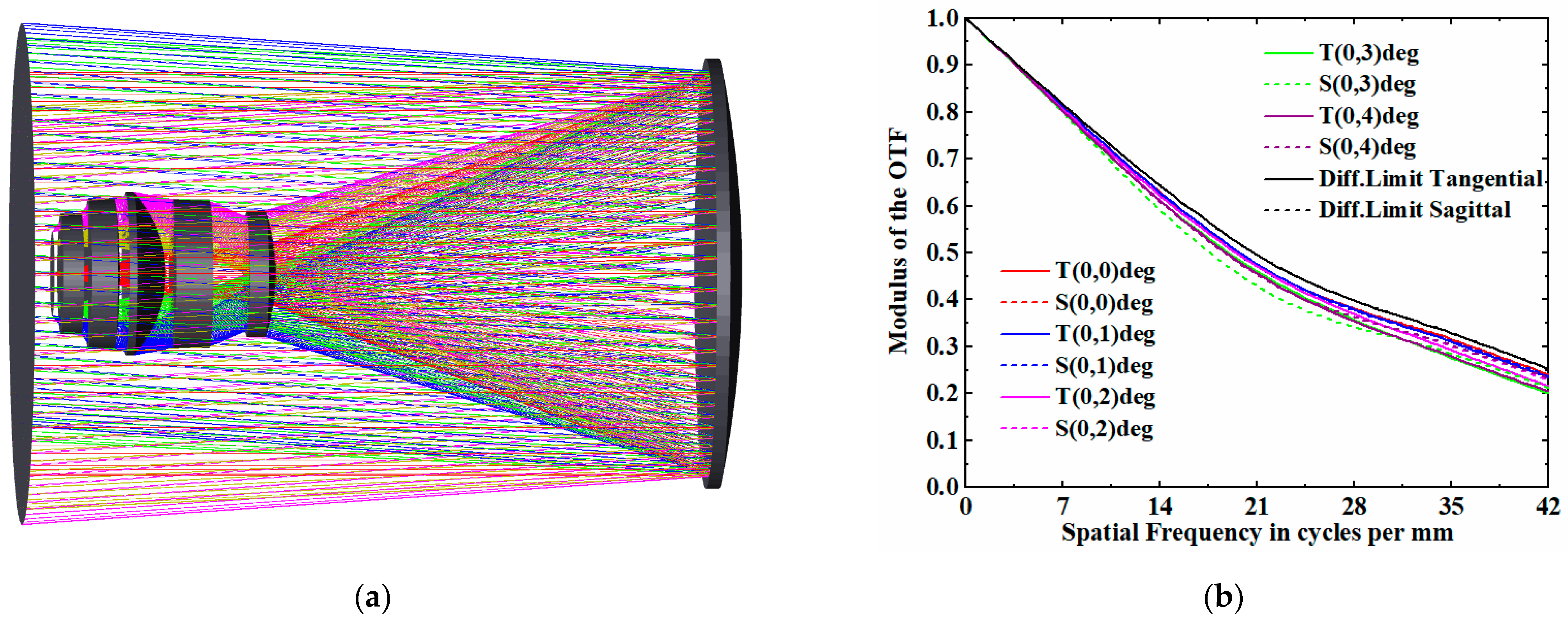
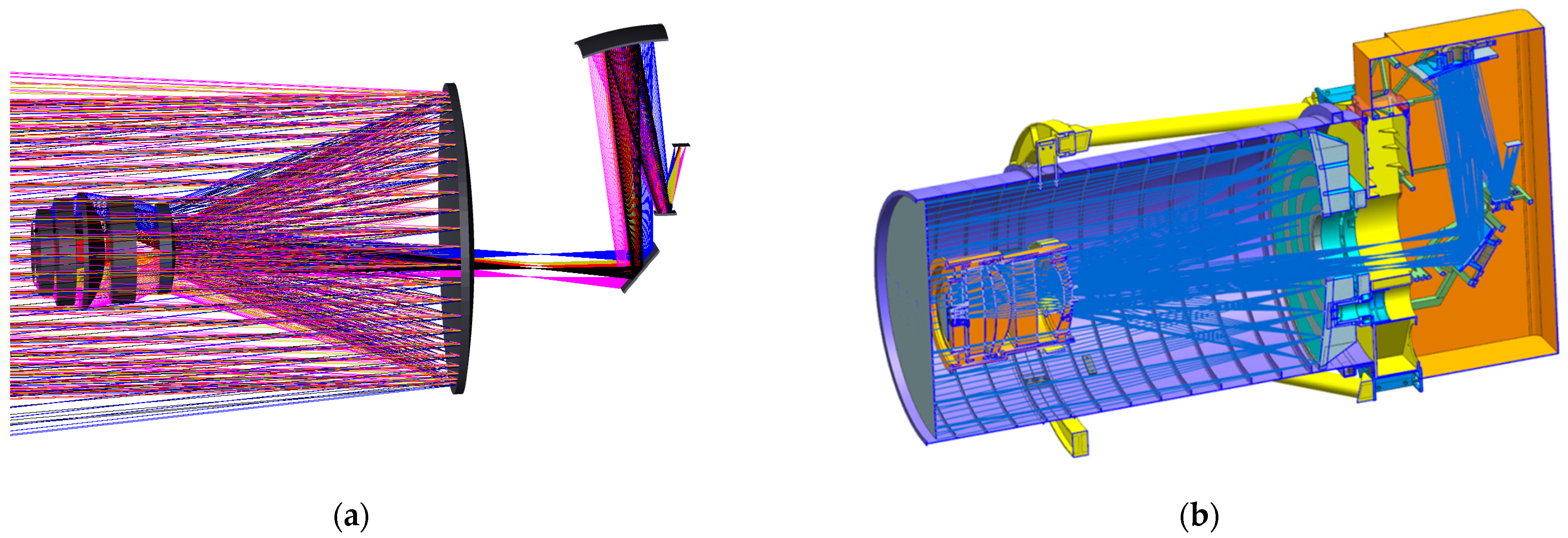
3.4. Overall Optical System

We combined the fore-infrared lens and relayed the germanium mirror and rear-polarization mirror into an overall system, and the optical layout is shown in Figure 9a. The final overall optical imaging system has an intermediate image plane, of which, the whole light paths share a primary mirror. The primary and secondary mirrors make a typical RC optical system, where the primary reflector is the aperture diaphragm of the system, and the primary and secondary mirrors are spherical with conic coefficients. The secondary mirror is set coaxially with the germanium mirror. It is coated with a high-reflectance film designed for a 0.45–0.9 μm band, which transmits long-wave infrared light while reflecting visible and near-infrared light. Moreover, the light path is divided into visible/near-infrared and long-wave infrared branches. The folded common-shared field of view can be divided into two independent fields of view after the view of the optical system is reflected by the secondary mirror, in which the long-wave infrared branch is a symmetrical square field of view, and the visible/near-infrared panchromatic polarization is an off-axis rectangular field of view. In addition, the total axial length of the overall system was about 120 mm. The final opto-mechanical structure is shown in Figure 9b. The layout stop and inner cover are set to effectively eliminate the stray light, and eco-unfriendly materials will be significantly reduced at the same time.

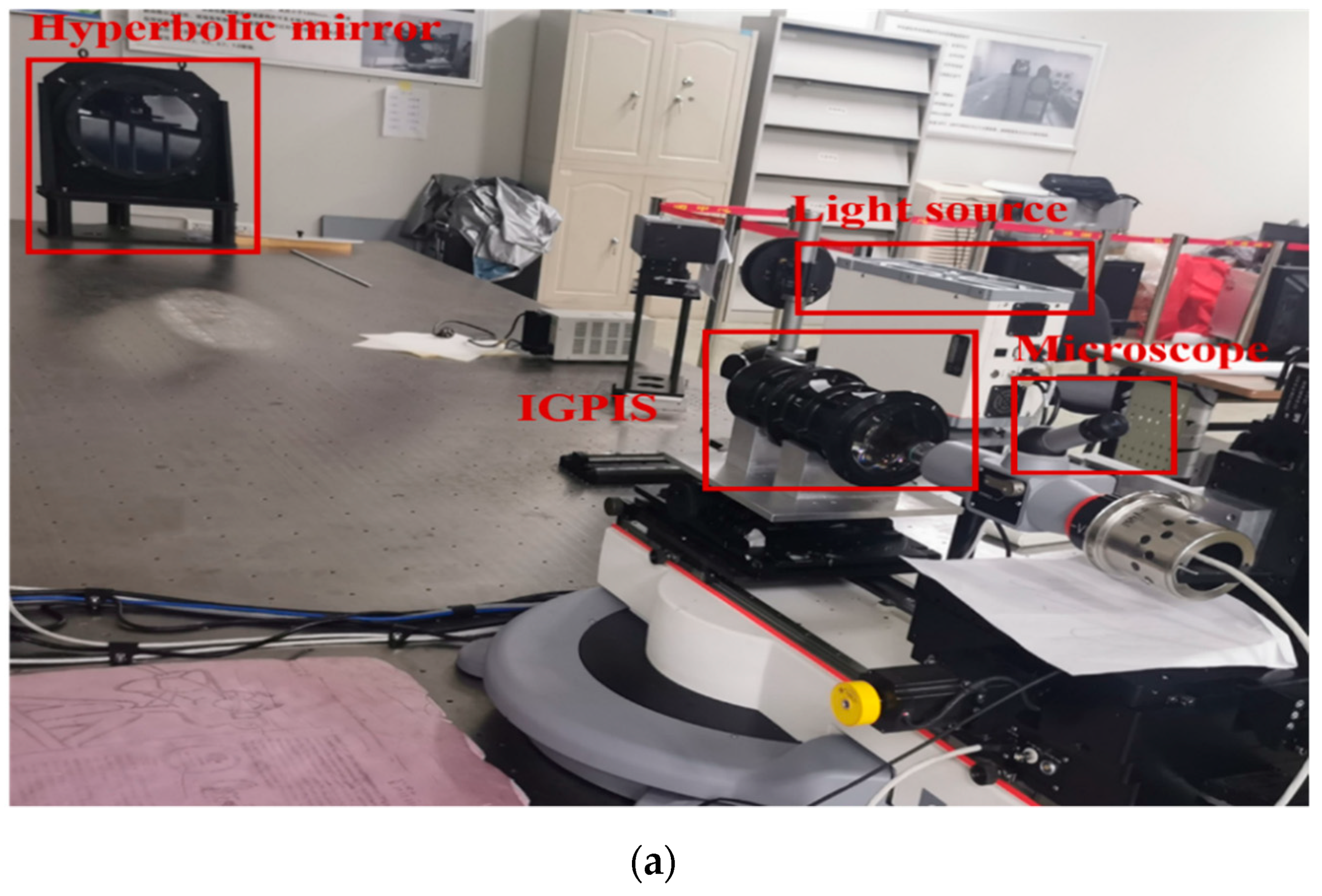
4. Ground Imaging Experiment

The IGIPS system is used for the common-aperture camera, and its imaging ability and image capturing performance need to be further verified. We built a MTF test experiment under laboratory conditions. As shown in Figure 10a, the entire experiment consists of a light source, target, hyperbolic mirror, camera, microscope, image transmitter-receiver and a computer terminal. First of all, we place the IGPIS camera on the optical stage, which is coaxial with the hyperbolic mirror. Then, a hyperbolic mirror is used to provide the camera with an infinite light source target that is imaged on the sensors. The actual spot shape can be observed through a microscope. Finally, a computer terminal will display the MTF value of the system. In fact, MTF > 0.1 is regarded as good imaging quality when a remote sensing camera is used. As shown in Figure 10b, the design MTF value of the rear-polarization system is 0.34, and the measured dynamic MTF value is 0.24; as shown in Figure 10c, the design MTF value of the rear-infrared system is 0.21, and the measured dynamic MTF value is 0.13. Therefore, IGPIS meets the requirements of remote sensing imaging.

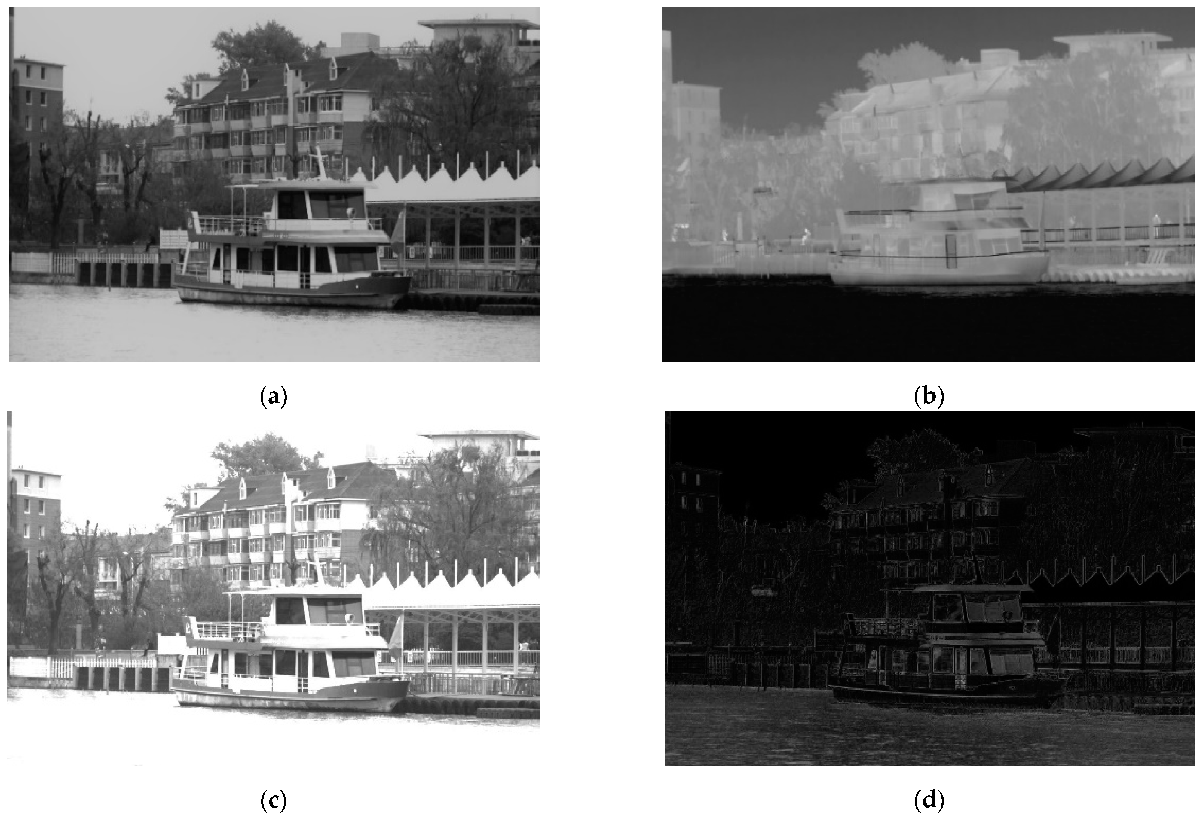
Outfield Imaging Experiment and Image Fusion

In order to verify the image capturing performance, it is necessary to establish an outfield experiment. The experiment was carried out in Nanhu Park, Changchun City, Jilin Province, China. Under the same conditions, the degree of polarization of water surface, glass and smooth wall is higher than that of rough backgrounds such as trees and roofs [29,30,31]. G.G. Stokes proposed the Stokes vector, which consists of four variables, S₀, S₁, S₂, S₃, and is used to describe the polarization state information of light waves [32]. An average Stokes vector can be decomposed into a sum of a completely polarized wave and a completely unpolarized wave. According to the principle, polarization imaging has been widely used in remote sensing imaging, such as synthetic aperture radar, imaging spectrometer, and space camera [33]. These four parameters are arranged into a column vector to measure the average light intensity over the duration, and then the Stokes vector light intensity is as follows:

$$S=\left[\begin{array}{l}{S}_0\\ S_1\\ S_2\\ S_3\end{array}\right]=\left[\begin{array}{l}{I}_0+I_{90}\\ I_0-I_{90}\\ I_{45}-I_{135}\\ I_R-I_L\end{array}\right]$$

(15)

where $S_0$ represents the orthogonal radiation intensity value of the light, $S_1$, $S_2$ and $S_3$ represent the polarization components of the three parameters in each direction, respectively.

Generally, the degree of linear polarization (DOLP) is as follows:

$$P_L=\frac{\sqrt{S_1^2+S_2^2}}{S_0^2}\times 100\%$$

(16)

where $p_L$ represents the percentage of the intensity of linearly polarized light to the total light.

Therefore, based on the polarization characteristics of the target, it is essential to perform polarization image pre-fusion in the transform domain. By extracting DOLP from images with different polarization angles, we establish the intensity coefficient matrix DP, which is utilized in fusion of image $S_0$ and image $S_{12}$ based on a wavelet transform. $S_0$ represents the first Stokes component, and $S_{12}$ is the L2 norm of the second and third stokes components. The core fusion rules of polarization imaging are as follows:

$$\underset{I_V}{\arg \min }DP\cdot \Vert I_V-S_{12}\Vert +(1-DP)\cdot \Vert I_V-S_0\Vert$$

(17)

in which, $I_V$ is a pre-fused image. We divide the image to be fused into four layers. The average weighted fusion is adopted in the low frequency part of the wavelet decomposition, and the fusion law was adopted in the high frequency part in Equation (17). Figure 11a,b are the original polarization and infrared images, respectively. The fused image and the linear polarization image are shown in Figure 11c,d, respectively.

There are some differences between the infrared system and the polarization system in the fields of view and focal lengths, so image registration is very important. Since the fact that the contour features are similar, the algorithm which matches the angular and azimuth features of the contour is adopted to realize the accurate registration of polarization and infrared images. Then the contour transformation matrix from polarization to infrared image is calculated to project. A point-to-point projection can be achieved by transforming the shapes of polarization images. As shown in Figure 12, the fusion rule of the infrared and polarized image are formulated by the weight of the pixel energy factor. A multi-level image decomposition method based on latent low-rank representation (MDLATLRR) is used to resolve the infrared and polarization images into the base and detail layers, respectively. Following this, the infrared base layer is regarded as the basic layer of the fusion image [34,35]. The infrared and polarized detail layers are superimposed on the detail layers of the fusion image by different weighting factors.

5. Discussion

The final fused image is shown in Figure 13. We highlight the IGPIS system ability of acquiring images and integrating multi-source information, and the infrared and polarization information are displayed on the fusion image by pseudo-color. The red section represents the distribution of heat sources, and the blue section represents the objects with polarization characteristics. By observing the whole pseudo-color image, the target with outstanding infrared and polarization features can be quickly found. The water surface, the glass and the roof of the boats that have obvious polarization characteristics are bluish, while the red and yellow thermal colors clearly show the people and the sightseeing boat under distant sunlight. Therefore, the sightseeing boats on the water surface can be accurately and quickly identified based on the multi-band fusion.

The information entropy, contrast and sharpness of the fused image describe the advantages of the fused images more objectively. To test these different aspects of the fused image F, the information entropy (IE), standard deviation (SD) and average gradient (AG) are calculated, and each sub-image before fusion is used as the calculation control group. As shown in

Table 4. List of various indicators of the fusion image.

Parameters	IE	SD	AG
I0	6.03	88.96	6.44
I45	6.70	83.67	7.32
I90	6.62	79.58	7.35
I135	6.70	82.46	7.20
IV	6.82	66.21	6.07
IR	6.08	55.71	4.10
F	7.53	55.03	12.77

, where $I_0$, $I_{45}$, $I_{90}$ and $I_{135}$ are images of polarization degrees of 0°, 45°, 90° and 135°, respectively and where $I_V$ and $I_R$ are the infrared and polarization images, respectively. Compared with each original image, the information entropy and average gradient of the fused image F are greatly improved, indicating that the fused image has richer details and contains more information. The standard deviation is lower, indicating that the brightness of the fusion image is more balanced, and the base layer is closer to the infrared image. These indicators show that the purpose of image fusion has been achieved.

6. Conclusions

In this paper, we presented an IGPIS to simultaneously achieve infrared and polarization detection of targets. On the basis of dynamic imaging theory, an IGP imaging mode is established for the common-aperture camera. The satellite attitude during the real-time guidance imaging process is analyzed by the quaternion method. We designed the overall optical system, which is composed of the fore-infrared, relay germanium, rear-polarization. It is a good attempt and innovation to realize the multi-band channels imaging and the miniaturized instrument by utilizing the transflective characteristic of relay germanium mirror. A principal prototype was built on our design. The results of outfield experiment further show that the infrared intensity information and polarization details information of targets are greatly preserved despite the influence of stray light. Compared with the single imaging instrument, our system can acquire the multi-dimension data cube within a single exposure, so it can be used for identifying dynamic targets, such as ships. The research provides a theoretical basis for a new mode of common-aperture imaging. In addition, IGPIS also has the potential of wide-area high-resolution observation of ground targets, which can be further studied.

References

1. Yang, M.; Xu, W.; Sun, Z.; Wu, H.; Tian, Y.; Li, L. Mid-wave infrared polarization imaging system for detecting moving scene. Opt. Lett. 2020, 45, 5884–5887. [Google Scholar] [CrossRef] [PubMed]
2. Bowles, J.H.; Korwan, D.R.; Montes, M.J.; Gray, D.J.; Gillis, D.B.; Lamela, G.M.; Miller, W.D. Airborne system for multispectral, multiangle polarimetric imaging. Appl. Opt. 2015, 54, F256–F267. [Google Scholar] [CrossRef] [PubMed]
3. Miyata, M.; Nakajima, M.; Hashimoto, T. Compound-eye metasurface optics enabling a high-sensitivity, ultra-thin polarization camera. Opt. Express 2020, 28, 9996–10014. [Google Scholar] [CrossRef] [PubMed]
4. Liu, M.; Yan, R.; Zhang, J.; Xu, Y.; Chen, P.; Shi, L.; Wang, J.; Zhong, S.; Zhang, X. Arctic Sea Ice Classification Based on CFOSAT SWIM Data at Multiple Small Incidence Angles. Remote Sens. 2021, 14, 91. [Google Scholar] [CrossRef]
5. Touzi, R. Target Scattering Decomposition in Terms of Roll-Invariant Target Parameters. IEEE Trans. Geosci. Remote Sens. 2006, 45, 73–84. [Google Scholar] [CrossRef]
6. Muhuri, A.; Manickam, S.; Bhattacharya, A. Scattering Mechanism Based Snow Cover Mapping Using RADARSAT-2 C-Band Polarimetric SAR Data. IEEE J. Sel. Top. Appl. Earth Obs. Remote Sens. 2017, 10, 3213–3224. [Google Scholar] [CrossRef]
7. Mura, A.; Adriani, A.; Sordini, R.; Sindoni, G.; Plainaki, C.; Tosi, F.; Filacchione, G.; Bolton, S.; Zambon, F.; Hansen, C.J.; et al. Infrared Observations of Ganymede from the Jovian InfraRed Auroral Mapper on Juno. J. Geophys. Res. Planets 2020, 125, e2020JE006508. [Google Scholar] [CrossRef]
8. Vizgaitis, J.N.; Hastings, A. Dual band infrared picture-in-picture systems. Opt. Eng. 2013, 52, 061306. [Google Scholar] [CrossRef]
9. Ohno, H. Multi-angle-view monocular camera using a polarization image sensor. Appl. Opt. 2019, 58, 4036–4041. [Google Scholar] [CrossRef]
10. Ding, Z.; Sun, C.; Han, H.; Ma, L.; Zhao, Y. Calibration Method for Division-of-Focal-Plane Polarimeters Using Nonuniform Light. IEEE Photonics J. 2021, 13, 3900309. [Google Scholar] [CrossRef]
11. Ratliff, B.M.; LeMaster, D.A.; Mack, R.T.; Villeneuve, P.V.; Weinheimer, J.J.; Middendorf, J.R. Detection and tracking of RC model aircraft in LWIR microgrid polarimeter data. Proc. SPIE-Int. Soc. Opt. Eng. 2011, 8160, 25–31. [Google Scholar]
12. Baumann, B.; Götzinger, E.; Pircher, M.; Hitzenberger, C.K. Single camera based spectral domain polarization sensitive optical coherence tomography. Opt. Express 2007, 15, 1054–1063. [Google Scholar] [CrossRef] [PubMed] [Green Version]
13. Fei, H.; Li, F.-M.; Chen, W.-C.; Zhang, R.; Chen, C.-S. Calibration method for division of focal plane polarimeters. Appl. Opt. 2018, 57, 4992–4996. [Google Scholar] [CrossRef] [PubMed]
14. Li, N.; Zhao, Y.; Pan, Q.; Kong, S.G. Demosaicking DoFP images using Newton’s polynomial interpolation and polarization difference model. Opt. Express 2019, 27, 1376–1391. [Google Scholar] [CrossRef]
15. Yang, T.; Jin, G.-F.; Zhu, J. Automated design of freeform imaging systems. Light. Sci. Appl. 2017, 6, e17081. [Google Scholar] [CrossRef]
16. Liang, J.; Zhang, W.; Ren, L.; Ju, H.; Qu, E. Polarimetric dehazing method for visibility improvement based on visible and infrared image fusion. Appl. Opt. 2016, 55, 8221. [Google Scholar] [CrossRef]
17. Fang, S.; Xia, X.; Huo, X.; Chen, C. Image dehazing using polarization effects of objects and airlight. Opt. Express 2014, 22, 19523–19537. [Google Scholar] [CrossRef]
18. Lu, H.; Zhao, K.; You, Z.; Huang, K. Real-time polarization imaging algorithm for camera-based polarization navi-gation sensors. Appl. Opt. 2017, 56, 3199–3205. [Google Scholar] [CrossRef]
19. Lu, H.; Zhao, K.; Wang, X.; You, Z.; Huang, K. Real-time Imaging Orientation Determination System to Verify Imaging Polarization Navigation Algorithm. Sensors 2016, 16, 144. [Google Scholar] [CrossRef] [Green Version]
20. Jiang, L.; Yang, X. Study on Enlarging the Searching Scope of Staring Area and Tracking Imaging of Dynamic Targets by Optical Satellites. IEEE Sens. J. 2021, 21, 5349–5358. [Google Scholar] [CrossRef]
21. Tangpattanakul, P.; Jozefowiez, N.; Lopez, P. A multi-objective local search heuristic for scheduling Earth observations taken by an agile satellite. Eur. J. Oper. Res. 2015, 245, 542–554. [Google Scholar] [CrossRef] [Green Version]
22. Huang, C.; Chang, Y.; Xiang, G.; Han, L.; Chen, F.; Luo, D.; Li, S.; Sun, L.; Tu, B.; Meng, B.; et al. Polarization measurement accuracy analysis and improvement methods for the directional polarimetric camera. Opt. Express 2020, 28, 38638–38666. [Google Scholar] [CrossRef] [PubMed]
23. Huang, E.; Ma, Q.; Liu, Z. Ultrafast Imaging using Spectral Resonance Modulation. Sci. Rep. 2016, 6, 25240. [Google Scholar] [CrossRef]
24. Brueckner, A.; Duparré, J.; Leitel, R.; Dannberg, P.; Bräuer, A.; Tünnermann, A. Thin wafer-level camera lenses inspired by insect compound eyes. Opt. Express 2010, 18, 24379–24394. [Google Scholar] [CrossRef]
25. Gong, T.; Jin, G.; Zhu, J. Point-by-point design method for mixed-surface-type off-axis reflective imaging systems with spherical, aspheric, and freeform surfaces. Opt. Express 2017, 25, 10663. [Google Scholar] [CrossRef]
26. Xu, T.; Yang, X.; Xu, C.; Chang, L.; Zhu, L. Study of satellite imaging with pitch motion compensation to increase SNR. Optik 2019, 192, 162933. [Google Scholar] [CrossRef]
27. Nieke, J.; Solbrig, M.; Neumann, A. Noise contributions for imaging spectrometers. Appl. Opt. 1999, 38, 5191–5194. [Google Scholar] [CrossRef]
28. Issa, V.; Daya, Z.A. Modeling the ship white water wake in the midwave infrared. Appl. Opt. 2018, 57, 10125–10134. [Google Scholar] [CrossRef] [PubMed]
29. Shuai, T.; Sun, K.; Wu, X.N.; Zhang, X.; Shi, B.H. A ship target automatic detection method for high-resolution remote sensing. In Proceedings of the IGARSS 2016—2016 IEEE International Geoscience and Remote Sensing Symposium, Beijing, China, 10–15 July 2016; pp. 1258–1261. [Google Scholar]
30. Han, J.; Moradi, S.; Faramarzi, I.; Liu, C.; Zhang, H.; Zhao, Q. A Local Contrast Method for Infrared Small-Target Detection Utilizing a Tri-Layer Window. IEEE Geosci. Remote Sens. Lett. 2020, 17, 1822–1826. [Google Scholar] [CrossRef]
31. Li, G.; Lin, Y.; Qu, X. An infrared and visible image fusion method based on multi-scale transformation and norm optimization. Inf. Fusion 2021, 71, 109–129. [Google Scholar] [CrossRef]
32. Stokes, G.G. On the Composition and Resolution of Streams of Polarized Light from different Sources. Trans. Camb. Philos. Soc. 1851, 9, 399. [Google Scholar]
33. Bhattacharya, A.; De, S.; Muhuri, A.; Surendar, M.; Venkataraman, G.; Das, A. A new compact polarimetric SAR decomposition technique. Remote Sens. Lett. 2015, 6, 914–923. [Google Scholar] [CrossRef]
34. Chen, G.; Li, L.; Jin, W.; Zhu, J.; Shi, F. Weighted sparse representation multi-scale transform fusion algorithm for high dynamic range imaging with a low-light dual-channel camera. Opt. Express 2019, 27, 10564–10579. [Google Scholar] [CrossRef] [PubMed]
35. Chen, Y.; Wang, L.; Sun, Z.B.; Jiang, Y.D.; Zhai, G.J. Fusion of color microscopic images based on bidimensional empirical mode decomposition. Opt. Express 2010, 18, 21757–21769. [Google Scholar] [CrossRef] [PubMed]
Figure 1. Principle diagrams of infrared-guided polarization imaging. (a) schematic diagram of infrared-guided polarization imaging. (b) schematic diagram of the satellite maneuvering path.
Remotesensing 14 01620 g001
Figure 2. Pixel-level polarization sensor. (a) principle and the layered structure within sensor. (b) one example of micro-polarization-pixel arrays.
Remotesensing 14 01620 g002
Figure 3. (a) The overlap area of the moved pupil and the original pupil. (b) the relation curve between the ρ 0 and the H ( ρ = 144 ) and the relation curve between the ρ 0 and the H ( ρ = 42 ) .
Remotesensing 14 01620 g003
Figure 4. (a) Optical layout of the fore-infrared system. (b) modulation transfer function of the fore-infrared system.
Remotesensing 14 01620 g004
Figure 5. (a) Spot diagram of the fore-infrared system. (b) field curvature of the different wavelengths. (c) distortion of the different wavelengths.
Remotesensing 14 01620 g005
Figure 6. The schematic diagram of the initial structure of the four-reflection optical system.
Remotesensing 14 01620 g006
Figure 7. (a) Optical layout of the rear-polarization system (b) modulation transfer function of the rear-polarization system.
Remotesensing 14 01620 g007
Figure 8. (a) Spot diagram of the rear-polarization system. (b) field curvature of the different wavelengths. (c) distortion of the different wavelengths.
Remotesensing 14 01620 g008
Figure 9. (a) The optical system three-dimensional layout of the common-aperture camera. (b) the opto-mechanical layout of the common-aperture camera.
Remotesensing 14 01620 g009
Figure 10. (a) MTF test principle prototype. (b) the MTF result of the rear-polarization system. (c) the MTF result of the fore-infrared system.
Remotesensing 14 01620 g010aRemotesensing 14 01620 g010b
Figure 11. (a) The original polarization image S0. (b) the original infrared image. (c) the polarization fused image. (d) the degree of linear polarization image.
Remotesensing 14 01620 g011
Figure 12. Flow chart of the infrared-polarization fusion imaging.
Remotesensing 14 01620 g012
Figure 13. (a) Fusion grayscale image. (b) pseudo-color enhancement image (red indicates infrared highlighting, blue indicates polarization highlighting).
Remotesensing 14 01620 g013