Enhancing the Accuracy and Temporal Transferability of Irrigated Cropping Field Classification Using Optical Remote Sensing Imagery

Abstract

Mapping irrigated areas using remotely sensed imagery has been widely applied to support agricultural water management; however, accuracy is often compromised by the in-field heterogeneity of and interannual variability in crop conditions. This paper addresses these key issues. Two classification methods were employed to map irrigated fields using normalized difference vegetation index (NDVI) values derived from Landsat 7 and Landsat 8: a dynamic thresholding method (method one) and a random forest method (method two). To improve the representativeness of field-level NDVI aggregates, which are the key inputs in our methods, a Gaussian mixture model (GMM)-based filtering approach was adopted to remove noncrop pixels (e.g., trees and bare soils) and mixed pixels along the field boundary. To improve the temporal transferability of method one we dynamically determined the threshold value to account for the impact of interannual weather variability based on the dynamic range of NDVI values. In method two an innovative training sample pool was designed for the random forest modeling to enable automatic calibration for each season, which contributes to consistent performance across years. The irrigated field mapping was applied to a major irrigation district in Australia from 2011 to 2018, for summer and winter cropping seasons separately. The results showed that using GMM-based filtering can markedly improve field-level data quality and avoid up to 1/3 of omission errors for irrigated fields. Method two showed superior performance, exhibiting consistent and good accuracy (kappa > 0.9) for both seasons. The classified maps in wet winter seasons should be used with caution, because rainfall alone can largely meet plant water requirements, leaving the contribution of irrigation to the surface spectral signature weak. The approaches introduced are transferable to other areas, can support multiyear irrigated area mapping with high accuracy, and significantly reduced model development effort.

1. Introduction

Globally, irrigated agriculture plays an important role in supporting agricultural production; however, water availability in the irrigation sector is limited due to hydrological factors, competing demands and the impact of climate change [1,2]. Water use efficiency is also low, at approximately 50% worldwide [3]. Consequently, good planning and management are of great importance to support sustainable development in irrigated agriculture and secure food supply. Monitoring the performance of irrigation is an important component of efficient irrigation management, which is assisted by accurate irrigated area mapping. An irrigated area map is a fundamental input to understand irrigation water demand, water allocation and efficiency. It is also one of the critical inputs to hydrological modeling, water budgeting and decision making [2,4,5].

Remote sensing is useful for irrigated area mapping over large regions because it provides comprehensive spatial data at relatively affordable costs in addition to global coverage [6]. Many papers have reported that irrigated areas can be successfully mapped using different types of satellite instruments, such as optical sensors [4,7,8], and microwave instruments, such as synthetic aperture radar (SAR) sensors [9,10,11]. When using optical data, irrigated fields can be mapped by using a single representative snapshot at the critical time (e.g., during peak season) or time series of images across the crop growing season [6]. Due to the seasonal nature of cropping practices, many classification methods use time series data to inform the irrigation status of individual fields. Inputs to classifications are commonly raw reflectance bands or multispectral indices that describe the distinctive features of irrigated fields. Normalized difference vegetation index (NDVI) is perhaps the most popular choice because (1) it has a good representation of green biomass that changes with the growth of crops; (2) it is an easily accessible indicator that can be generated from a wide range of optical satellites, including the CubeSats (e.g., PlanetScope constellation), with minimal bands; and (3) it is a normalized indicator that reduces the dependence on atmospheric calibration [12,13]. Numerous papers have proved the effectiveness of using NDVI time series in irrigated area mapping all over the world [7,14,15]. However, most existing irrigated area mapping studies have two key limitations when they are applied to large regions that involve a large number of fields and/or over multiple years: they lack good resampling methods of pixel-scale data to improve field-level data quality and they lack temporally transferable methods to avoid errors due to interannual climatic variability in multiyear classification.

While pixel-scale NDVI values are commonly used in classification, aggregating pixel-scale NDVIs to the field scale can improve classification results. In contrast to pixel-scale classification, which often leads to fragment classification results (known as the “pepper and salts” problem), field-scale analysis delineates field boundaries as a prior step so that irrigated areas can be displayed on “real object” (fields) [16,17,18]. Although there is an increasing trend towards field-scale analyses for practical considerations [19], limited attention has been paid to the potential errors introduced when aggregating pixel-scale data to the field scale. In particular, most studies have used all pixels within a field to calculate field-average data, assuming that agricultural fields are homogenous. In reality, each cropping field is heterogeneous, with multiple types of objects in the field [4,20,21,22]. Subfield-scale variabilities caused by noncrop patches, such as pixels from bare soil patches, trees and buildings, as well as mixed pixels at field boundaries can be included in the field-scale aggregation when all the pixel values within the field boundary are used, leading to representativeness errors in field-scale aggregation. A few papers attempted to minimize the effect of non-representative pixels in individual fields using different filtering approaches [23,24,25]. For example, Conrad et al. [23] evaluated the field boundary quality to avoid the accidental inclusion of pixels from the neighboring areas. De Castro et al. [25] only used pixels that are completely within the fields or pixels that have at least 50% overlapping area with the field for aggregation. However, most existing filtering methods rely on simple thresholds to screen out nonirrigation or noncropping pixels. One exception is Park et al. [26], who used Gaussian mixture modeling to separate tree canopies and intertree spaces (i.e., soil, ground cover) in a horticultural field. Such filtering essentially selects representative pixels for inclusion in canopy-scale or field-scale analyses, but there has been no study in irrigated field classification that used model-based methods to automatically select in-field representative pixels.

Another common challenge in irrigated field mapping is the development of a classification scheme that is robustly applicable to multiple years without manual parameter tuning. Routine irrigated area monitoring is important for supporting multiyear irrigation management due to the highly dynamic nature of irrigated areas in many regions. Most published methods are designed to work over a short period (i.e., a single year or a single season), with limited applicability to mapping dynamic field conditions over multiple years [5,27]. Classification schemes developed under a certain time may not be suitable for other times in the same area due to a variety of factors, such as the changing climate [27]. The district-level mixture of irrigated and nonirrigated areas is particularly variable in response to interannual climate variations, and this can confuse classifiers. Some papers have used a long-term average method to avoid recalibration [28]. Other papers attempted to improve multiyear classification accuracy by developing innovative input variables [27] or by combining training samples from multiple years for the development of a comprehensive method/model [5]. However, there is a general lack of systematic methods for performing automated classification across multiple years/seasons under varying hydroclimatic conditions.

Motivated by the above limitations in irrigated field classification, this work presents a statistical resampling method for field-scale pixel aggregation as well as two dynamic classification methods to enhance the accuracy of irrigated field classification across years. Time series of NDVI data and seasonal summaries of NDVI time series (NDVI metrics) from Landsat were used as the inputs for the classification methods. The two key innovations of this study are developing (1) a Gaussian mixture model (GMM)-based filtering method that can automatically select representative pixels at individual fields to improve the representativeness of input data for classification; (2) two temporally dynamic methods for multiyear classification, both of which outperform a temporally static method used as a comparator. The study was conducted in a modernized irrigation region—Coleambally Irrigation Area (CIA)—in Australia from 2011 to 2018. The GMM-based filtering method is applicable to any field-scale studies to improve the quality of input data, and the temporally dynamic modeling framework is transferred to other irrigation districts to benefit regional irrigation water management.

2. Materials and Methods

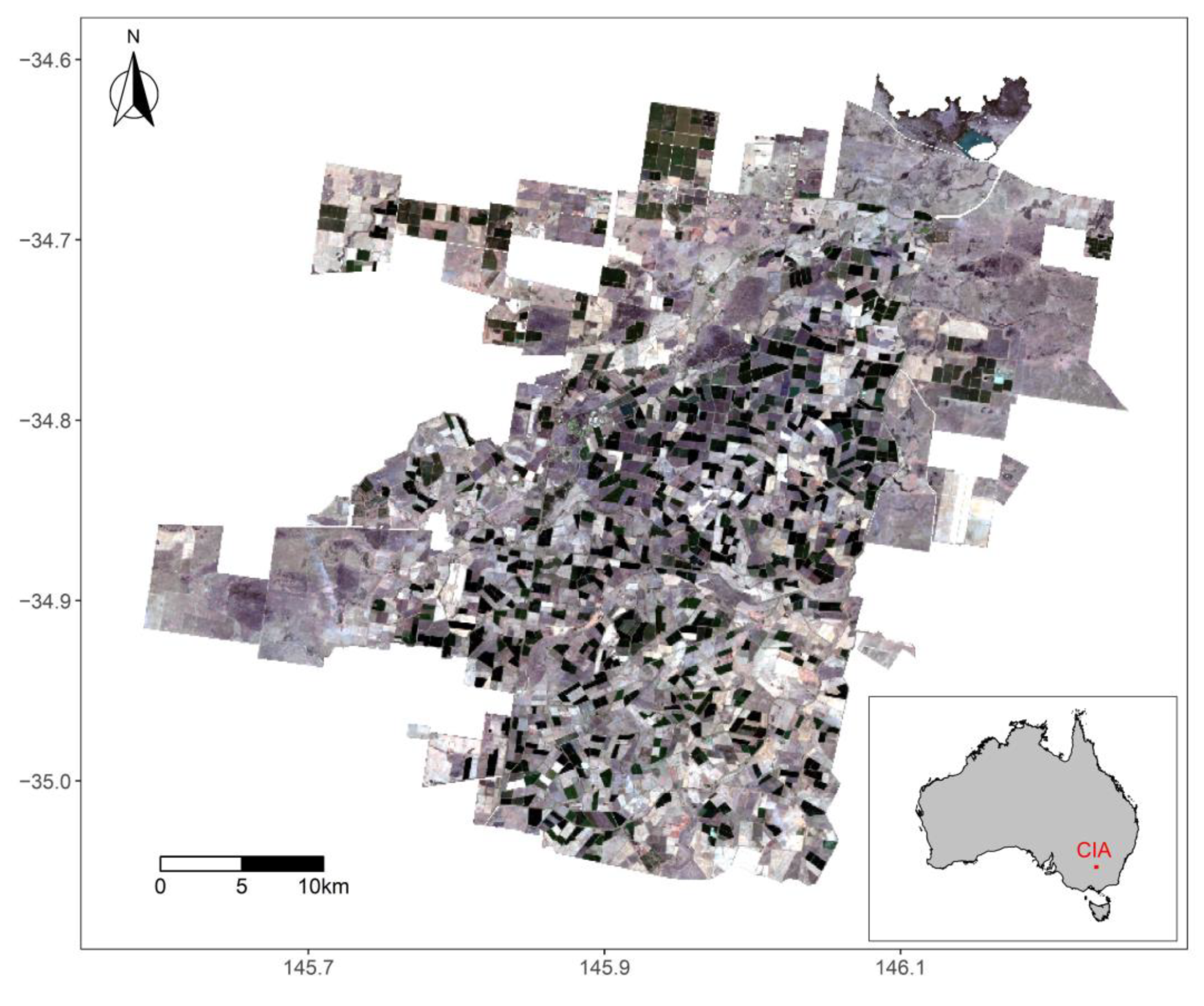
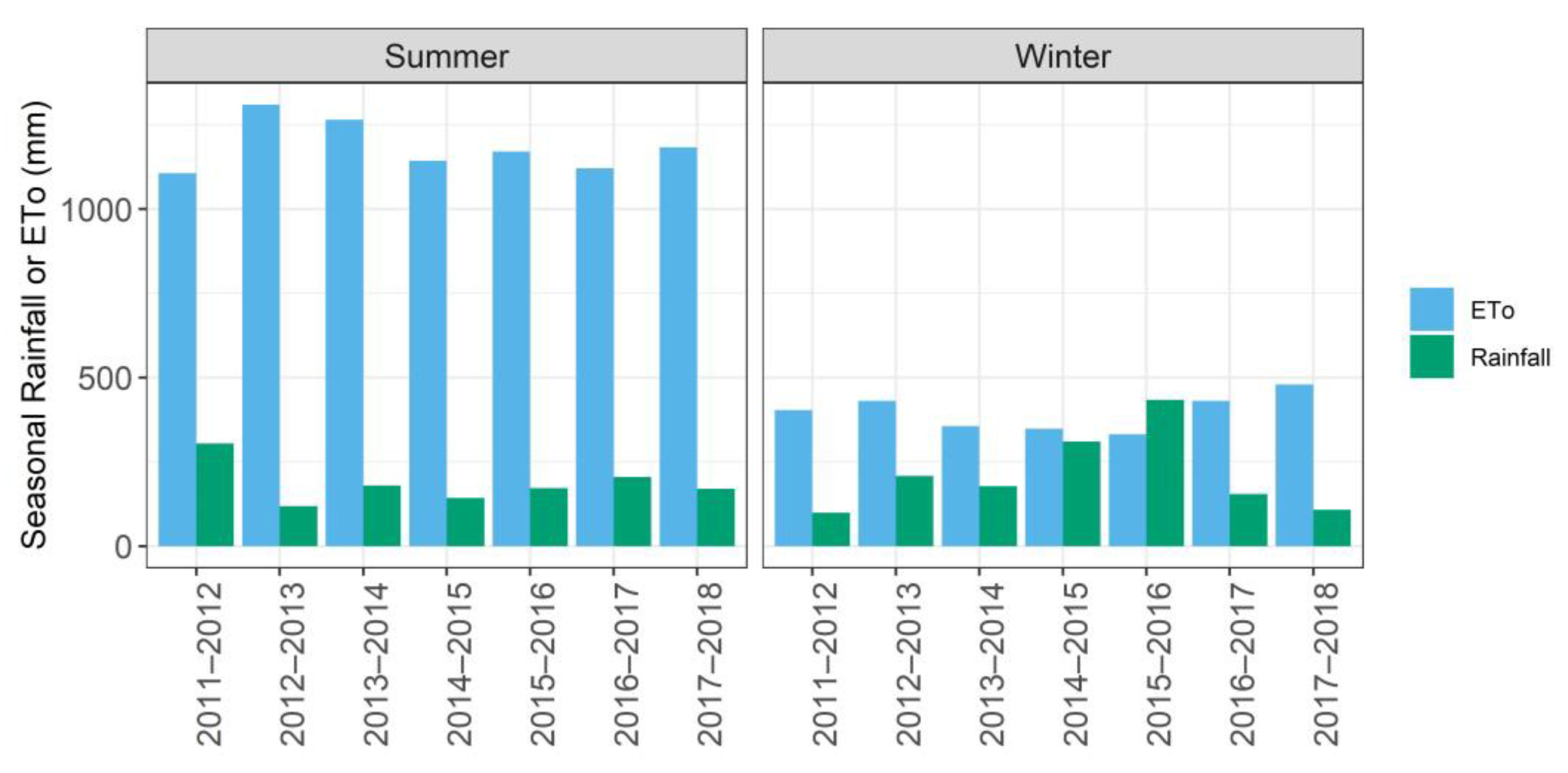
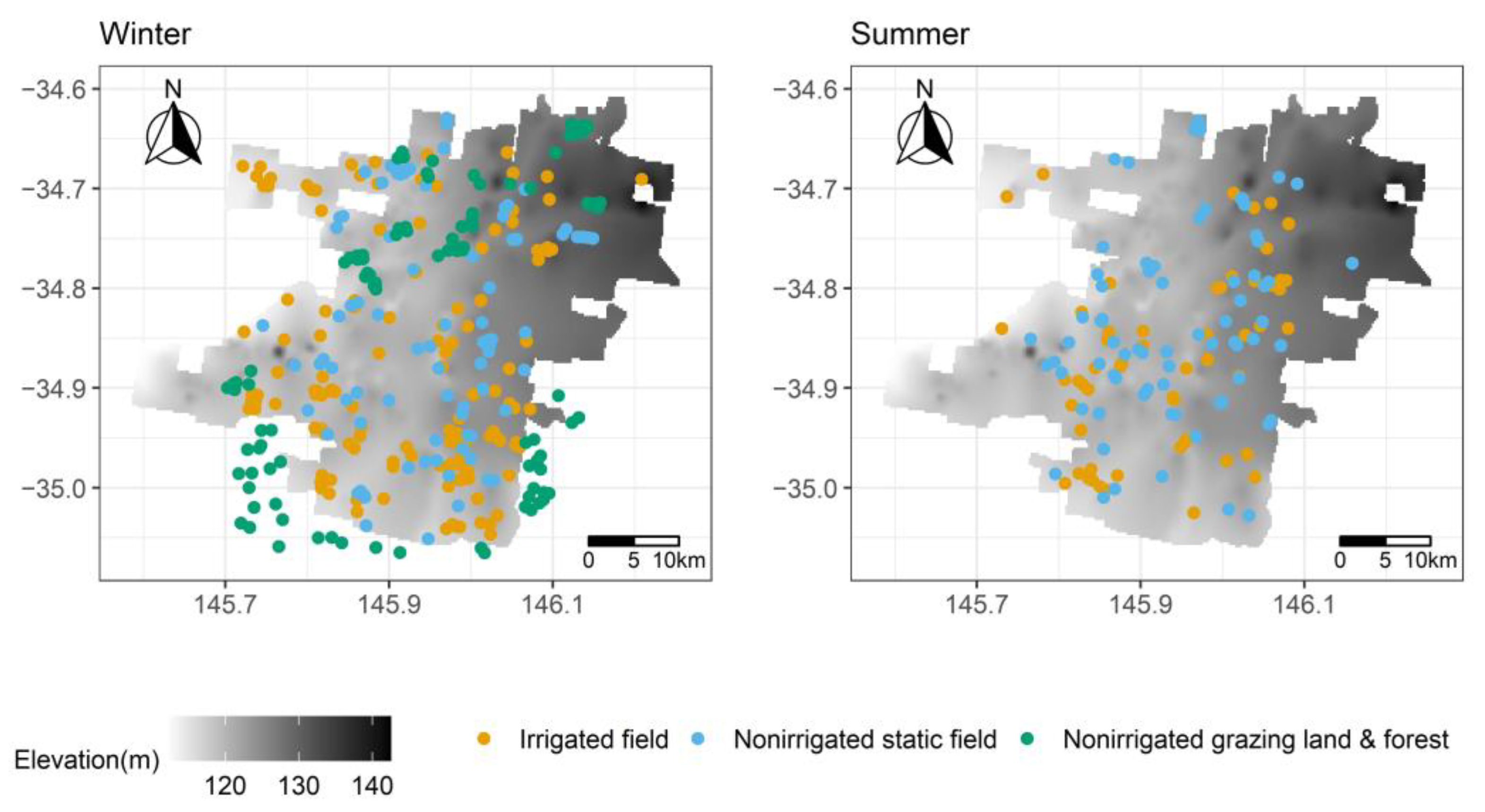
2.1. Study Area

The study area is the Coleambally Irrigation Area (CIA), a district with recently modernized and automated canal-based water delivery infrastructure, located in southern New South Wales, Australia (Figure 1). The district serves 79,000 hectares (ha) of irrigated land with approximately 500 farms, which have an average farm size of 220 ha. The use of dominant irrigated fields is for annual cropping, followed by pasture and irrigated fruit trees. State forests and individual trees are scattered across the region, and there are significant areas of dry-land grazing and cropping intermingled with the irrigated land. The main irrigation season is across spring–summer–autumn from mid-August to mid-May [29].

The cropping year is defined as the duration from the 1st of October to the 30th of September, although the winter cropping season may extend to the end of November. According to the local water utility, Coleambally Irrigation Co-operative Limited (CICL), three dominant types of annual cropping patterns of this region are the following: single summer cropping (October–April), single winter cropping (March–November) and double cropping (October–April, March–November). Typical annual summer crops include corn, cotton and rice, while typical winter crops are wheat, canola and barley. In addition, winter is the typical growing season for rainfed pasture. There are also a small number of farms growing perennial crops, such as almonds, wine grapes and citrus, in the CIA. The proportion of each crop type varies from year to year depending on many factors, such as water availability or crop prices (grower’s return) [30].

Figure 2 shows the seasonal rainfall and reference evapotranspiration (ETo) in the CIA, which were calculated using the daily ETo and rainfall obtained from the nearby Narrandera Airport weather station [31]. The average annual rainfall in the CIA is around 398 mm, with winter rainfall generally higher than summer rainfall, and there is substantial interannual variability [31]. The average summer ETo is 1186 mm, largely exceeding the average winter ETo, which is 397 mm. The long-term average temperature is 24 °C [31]. Due to the nature of the hot and dry summer in addition to the wetter and cool winter, summer crops in the CIA rely heavily on irrigation, while winter crops can be rainfed or supplementally irrigated.

Irrigation water in the CIA is delivered to farms from the Murrumbidgee river through the main channel and supply channels [32]. The actual amount of water delivered to a farm/field in each season is capped by water allocation (allowing for any trading between users), which is determined from the water availability in a given year. Water allocation is affected by streamflows and reservoir storages in the upstream catchments; therefore, water delivered to a farm varies from year to year. Surface irrigation is the most common irrigation method in the CIA [32].

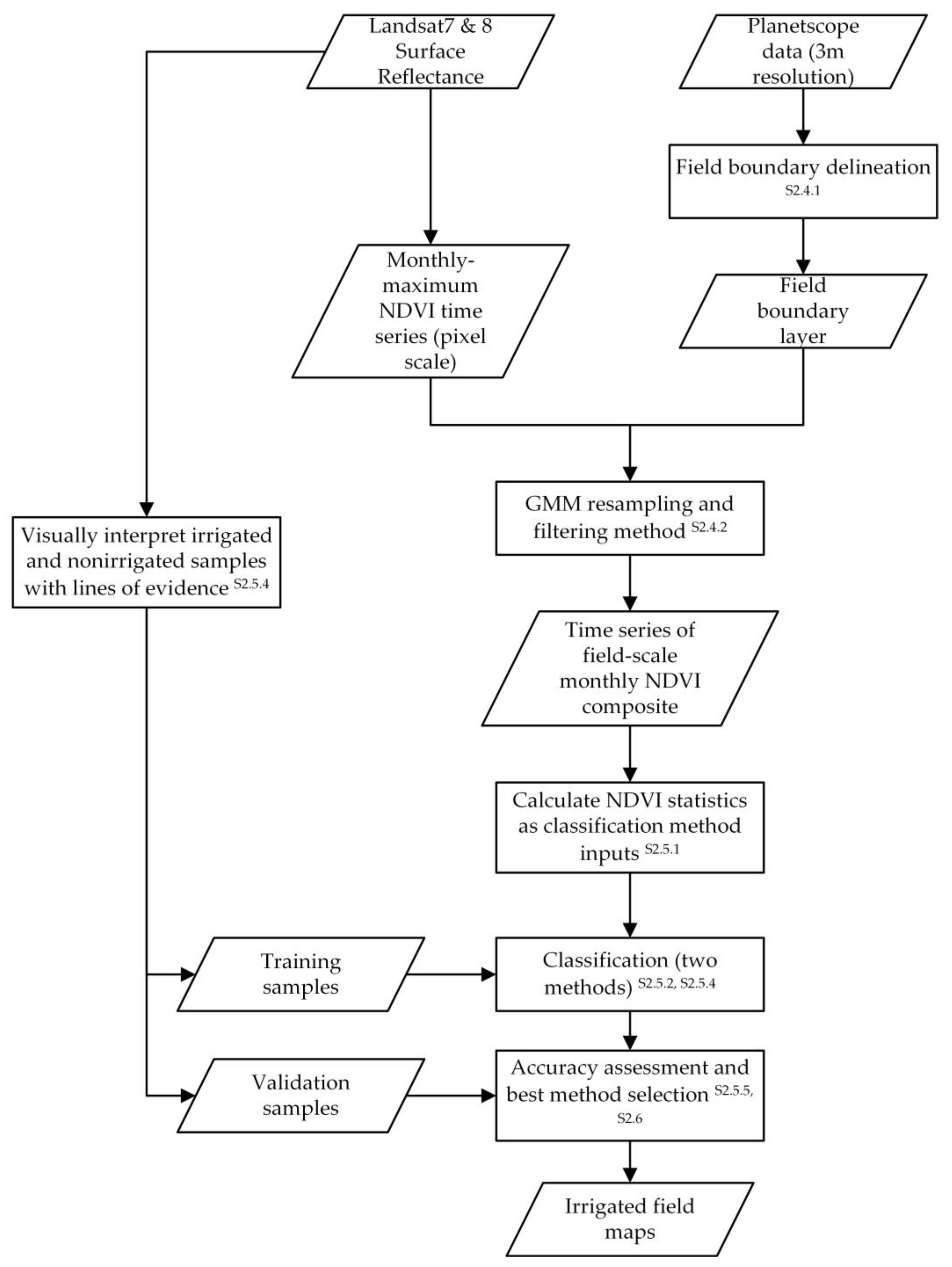
2.2. Research Overview

Figure 3 presents the methodology of this paper. We classified irrigated areas at the field scale—the typical management unit of land used for agricultural purposes with similar crop cultivars and irrigation management. We firstly delineated field boundaries using 3-m-resolution PlanetScope data. Monthly Landsat 7 and 8 data were aggregated by field to reproduce temporal changes in vegetation. Two different classification methods were developed and evaluated, from which the best-performing method was selected to classify fields for the entire study region.

2.3. Data

2.3.1. Satellite Data

We used very-high-resolution satellite imagery (3 m) to delineate field boundaries (Section 2.4.1). The composite image was derived from the Level 3B product of PlanetScope, acquired on 30 August 2019, downloaded from the Planet Labs website [33]. Monthly Landsat NDVI data were extracted at the pixel scale for the period of 2011–2018. These were further filtered and aggregated to the field scale for classification (Section 2.4.2). Both Landsat 7 (USGS Landsat 7 Surface Reflectance Tier 1) and Landsat 8 (USGS Landsat 8 Surface Reflectance Tier 1) images were used to construct false-color composites for the visual inspection of training samples as well as to calculate pixel-scale NDVI data, which was performed using the Google Earth Engine cloud platform [34].

2.3.2. Ancillary Data—Farmer-Reported Cropping Areas

Farmer-reported cropping areas for each irrigated crop type were collected and managed by CICL. These data were used as an independent database with which to validate the satellite-based classified cropping areas.

2.4. Data Preprocessing

2.4.1. Field Boundary Delineation

Delineating field boundaries is a prerequisite for field-scale irrigated area classification. This is typically conducted by using either manual delineation or object-based image analysis (OBIA) methods applied to satellite images [35]. OBIA first transfers the pixels into small objects that are homogenous using image segmentation, and then further clusters these objects by their spectral, geometrical and spatial features [36,37]. The ideal resolution for satellite data for field boundary delineation is <10 m to ensure precision. Hence, we used the Planetscope image which has a 3 m resolution. Field boundaries were assumed to be static over the study period; therefore, the field boundary layer delineated using the Planetscope image on 30 August 2019 was used for all tested years.

The image segmentation was performed using the Feature Extraction (FX) module in ENVI [38], which applies edge-based watershed transform algorithms [39]. It is worth noting that the parameter settings of algorithms have a direct impact on boundary accuracy. Hence, inspired by Xu et al. [40], we used texture information, namely the gray-level cooccurrence matrix (GLCM), to inform the best segmentation parameters for individual fields. The essential idea is to explore the relationship between the GLCM variance and a key segmentation parameter: scale level in the FX module. The GLCM variance can then be used as an indicator to determine the optimal scale level for individual fields. Detailed segmentation procedures are explained in Section S1 (Figures S1 and S2 and Table S1) of the Supplementary Materials.

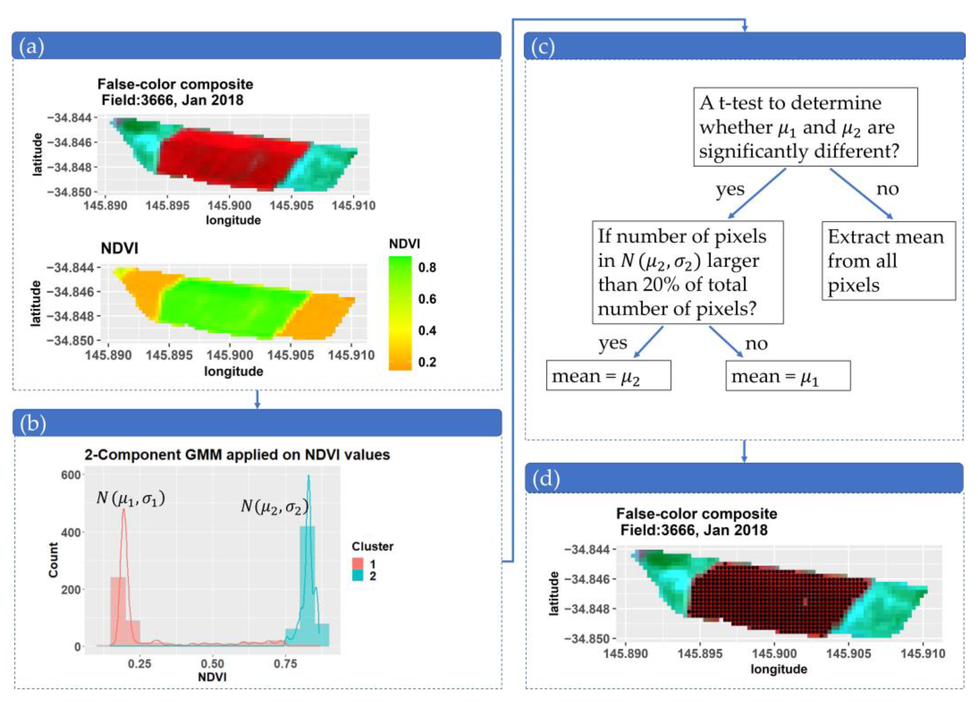
2.4.2. Field-Scale NDVI Filtering Using a Gaussian Mixture Model (GMM)

We used the normalized difference vegetation index (NDVI) [41] to separate irrigated and nonirrigated fields, as recommended by many previous works [4,13,14,15]. A more detailed justification for the use of the NDVI is provided in the Introduction section. The NDVI is calculated using the red and near-infrared bands, and is commonly used to represent green biomass, plant health and photosynthetic activity [42,43]. The assumption is that irrigated fields are covered by a higher level of green biomass once crops are established compared to nonirrigated fields. Landsat data were selected due to their good spatial detail (30 m resolution) and long record duration, which fully cover the study period. The typical 16-day return period of Landsat is halved over our study region, as the CIA is in an overlapping area of two Landsat scenes (row 92 and path 84 in addition to row 93 and path 84). A cloud mask was applied which removed pixels labeled as “Cloud” or “Cloud shadow” in the Land Surface Reflectance Code [44]. To reduce the impact of cloud-contaminated pixels we used the maximum composite values method to extract the maximum monthly NDVI [45]. Any missing data for individual pixels were linearly interpolated using the temporally neighboring monthly NDVI(s).

Field-scale NDVI values were derived by averaging the NDVI of representative pixels selected using a GMM-based filtering method for individual fields. Specifically, this filtering method was developed to select pixels that represent the actual field conditions and remove within-field noncrop pixels, such as bare soil patches and trees. The overall process is to (1) use the GMM to divide pixels into two clusters that hypothetically represent different clusters of objects X and Y (e.g., crop and bare soil patches), (2) determine which cluster is more representative for the field and (3) use pixels of the more representative cluster to calculate the field-average NDVI.

Figure 4 demonstrates the GMM-based filtering method using an example field in January 2018. The false-color composite shows the heterogeneity within the field, as crops only cover the center of the field and the rest is fallow land (Figure 4a). Without filtering, the field-average NDVI would be significantly reduced by the nonirrigated pixels displayed in green in the false-color composite. A two-component Gaussian mixture model (GMM) was thus applied to all NDVI values within the field, and thereby divided them into two distributions (Figure 4b). A GMM is a probabilistic model that automatically assigns observations to a predefined number of clusters (also called “component”, or k), assuming observations in each cluster following the normal distribution [46]. We chose a bimodal distribution (i.e., k = 2) because we assumed that pixels belong to either nonirrigated or irrigated populations.

A t-test was subsequently applied to the two-component GMM with component distributions of $N\left({\mu }_1,{\sigma }_1\right)$ and $N\left({\mu }_2,{\sigma }_2\right)$ to determine how statistically distinct the two populations were (Figure 4c). The null hypothesis was that ${\mu }_1$ = ${\mu }_2$, that is, the pixel values were from a single population. If the null hypothesis (p < 0.05) was rejected we concluded that irrigated and nonirrigated pixels coexist, and GMM-based filtering is required. We then selected the higher mean (${\mu }_2$) as the field-scale NDVI, provided the number of pixels in $N\left({\mu }_2,{\sigma }_2\right)$ exceeds 20% of the total number of pixels. Normally this representative Gaussian distribution has more than 50% of the total pixels, but here we set a lower threshold of 20% to give priority to the distribution with a higher NDVI, while also ensuring that small clusters of trees or weeds and deceptively high NDVIs are not treated as irrigated. If the null hypothesis was accepted we assumed that the field is homogenous, with pixels from one population. In this case, the field-level NDVIs were extracted from all pixels. For the example in Figure 4, the GMM identified two clusters and identified the irrigated pixels, as shown with black dots in Figure 4d, demonstrating the ability of GMM-based filtering to reduce noise in the field-scale data.

2.5. Irrigated Field Classification

Decision-based classification methods are commonly used in irrigated field classification studies [5,7]. We developed two temporally dynamic classification methods to detect irrigated fields, both having the same basic building block—a decision tree—but using different strategies to make decisions. The first method (method one, the dynamic thresholding method) applied threshold-based decision trees with an annually changing threshold to classify irrigated and nonirrigated fields. The threshold was derived from the seasonal maximum NDVIs from all fields using a Gaussian mixture model and a density slicing function. The second method (method two, the random forest method) was developed using the random forest algorithm, which was trained using an innovative training sample pool that allows the classification rules to be updated for individual years. A baseline method (method—baseline) using the same structure of method one but with fixed thresholds was used for comparison. The baseline method is a temporally static model that is commonly applied in existing studies [7,47]. Comparisons against the baseline demonstrate the value of using temporally dynamic models in multiyear classification.

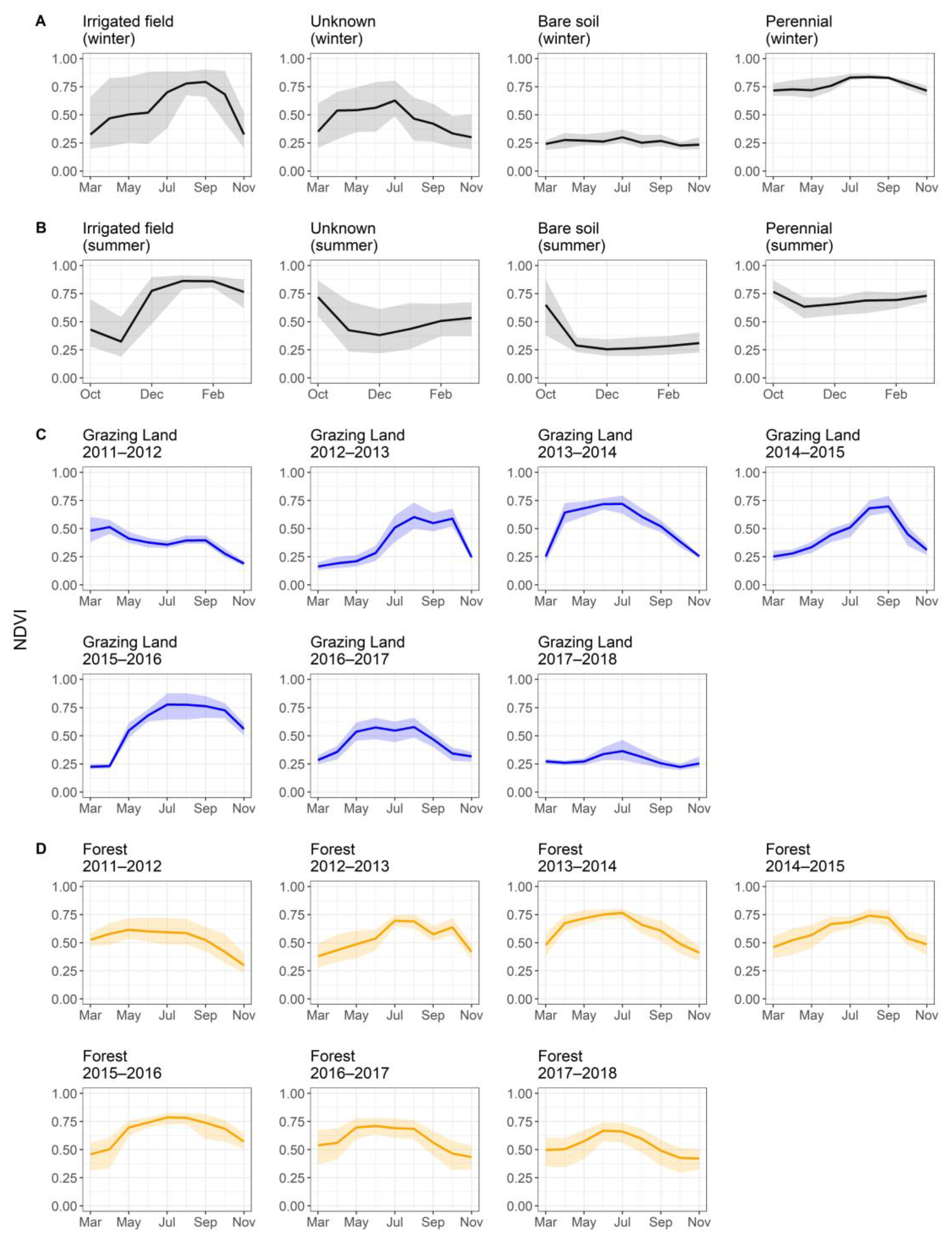
2.5.1. Model Inputs—NDVI Metrics

Selecting an appropriate seasonal summary of NDVI time series (NDVI metrics) is important to distinguish irrigated fields from nonirrigated fields. NDVI metrics were selected based on the premise that (1) irrigated cropping fields exhibit more intense green than nonirrigated fields and (2) irrigated fields have distinctive seasonal characteristics: a low NDVI at sowing and harvesting and a high NDVI at the peak season. Hence, in the thresholding methods (method one and method—baseline) two critical features, namely the seasonal maximum NDVI (abbreviation: MAX) and the NDVI range (abbreviation: RANGE), were used (

Table 1. Two critical NDVI features used in the thresholding methods.

Feature Name	Abbreviation	Description
The seasonal maximum NDVI	MAX	The maximum NDVI value within a season 1.
NDVI range	RANGE	The maximum NDVI minus the minimum NDVI. Note: if the minimum NDVI is less than 0.2, use 0.2.

¹ Maximum NDVI is extracted from December to February for summer and from June to October for winter.

).

We developed a set of NDVI metrics as model inputs for the random forest classification (method two). Method two can handle high dimensional problems [48]; therefore, a total of 14 NDVI inputs were used to help the method better understand the interclass and intraclass variation. These NDVI inputs include raw NDVI values and summaries of NDVI time series, such as the timing of the NDVI reaching a certain value or the maximum rate of increase in the NDVI. Detailed explanations of the 14 NDVI inputs are provided in Table S3 of the Supplementary Materials.

2.5.2. Dynamic Thresholding Method (Method One)

Method one (dynamic thresholding method) used a simple decision tree with thresholds applied to the MAX and RANGE to binarily classify fields (Figure 5). The threshold, α, for the MAX is determined dynamically across years to cater for interannual variations in the best separation point for irrigated and nonirrigated fields. This variation is primarily due to different weather conditions between years. The selection of α is described in detail below (step 1 to step 6). The RANGE threshold checks that the expected dynamic NDVI behavior of irrigated crops is present; that is, that the NDVI increases from near zero to a well-vegetated field before potentially declining. This eliminates fields with a constantly high NDVI, such as areas of trees. This threshold is set at a fixed value of 0.4.

The determination of α is summarized as follows:

Step 1: for a particular year, extract the seasonal maximum NDVI (MAX) for all fields.

Step 2: apply a Gaussian mixture model (GMM) with the number of components (k) selected based on the maximum Bayesian inference criteria (BIC) for models with k ranging from 2 to 9.

Step 3: resample all MAX values (all fields) into k components, with each component distributed as N(µ_i, σ_i), where i is the component number.

Step 4: calculate the 5% quantile of each cluster (left tail) and combine clusters whose 5% quantiles are above and below 0.6, respectively. The comparison with 0.6 is to further divide clusters into two populations to represent irrigated and nonirrigated fields. The use of the 5% quantile within each cluster assumes that if more than 95% of pixels in a cluster are above 0.6 (i.e., most of the fields in this cluster have reached a high NDVI within the season), the cluster represents irrigated fields.

Step 5: calculate the mean and standard deviation for the two groups from step 4 (µ_l,σ_l, µ_h,σ_h, where the subscripts l and h represent clusters’ 5% quantiles < 0.6 and >0.6, respectively).

Step 6: calculate the dynamic threshold using the density slicing function (1):

$$\alpha =\frac{{\mu }_l\cdot {\sigma }_h+{\mu }_h\cdot {\sigma }_l}{{\sigma }_l+{\sigma }_h}$$

(1)

2.5.3. The Baseline Method (Method—Baseline)

We also generated a baseline model (method—baseline) that inherits the same structure of method one but with fixed thresholds of both the MAX and RANGE. The method—baseline serves as a control test, whose performance is thus compared with method one to demonstrate the merit of using dynamic thresholds. The MAX and RANGE were set as 0.6 and 0.4, respectively, based on the manual inspection of arbitrarily chosen samples. This means that any field that has a seasonal maximum NDVI larger than 0.6 and an NDVI range larger than 0.4 was considered as an irrigated field.

2.5.4. The Random Forest Method (Method Two)

Method two used a popular machine learning algorithm—a random forest for classification. The random forest algorithm has been increasingly used in irrigated land classification due to its ability to handle high-dimensional data with good accuracy and efficiency [48,49]. The innovation in method two, compared to existing random forest classification methods, is that it was retrained each year using a training sample pool constructed to account for the impacts of changing weather conditions across years. Method two was implemented using the R package “randomforest” [50].

Training Samples

Method two, as a supervised classification, requires the selection of training samples for model development. Irrigated and nonirrigated samples were selected via the visual interpretation of satellite imageries. Visual interpretation is an efficient sample collection method compared to on-field collection, but the irrigation status requires verification using robust lines of evidence [5]. The auxiliary data used for visual interpretation included Landsat 8 false-color composites, monthly NDVI time series, very-high-resolution images on Google Earth and fieldtrip information. The overall procedures of sample selection were summarized as follows, and the detailed processes are provided in Section S2 in the Supplementary Materials.

This paper created a novel training sample pool, aiming to minimize the effort involved in sample collection while maintaining method two′s transferability across multiple years. One concern in multiyear classification is that the crop phenology (NDVI time series) for some samples varies dramatically across time, which makes a model trained in one year inapplicable for another [51]. One possible solution is to recalibrate the model using samples from different years, but the sample recollection and model recalibration is a time-consuming process. To solve this problem we first inspected the NDVI time series of samples from different classes to determine which class(es) have high variation between NDVI profiles across years. The classes that have consistent NDVI time series across years are called “static” classes, and they can be kept unchanged in the training sample pool. The classes for which NDVI time series change dramatically across years are called “dynamic” classes, and samples in these classes need to be updated when model training is applied in different years.

This paper designed 4 static classes (i.e., “irrigated cropping and pasture”, “unknown”, “bare soil” and “perennial plantation” (Figure 6A,B)) and two dynamic classes (i.e., “nonirrigated grazing land” and “forest” (Figure 6C,D)) based on observations of field-level NDVI time series and expert knowledge. It is worth noting that dynamic samples are only used for winter classification when nonirrigated grazing land and forest fields show irrigated-like features and could be potentially misclassified as irrigated fields. In summer, nonirrigated grazing land and forest fields are very similar to “bare soil” or “unknown”, so their samples were merged into these two classes rather than being established as separated classes.

Samples from the static classes, once collected within the CIA, were kept unchanged in the sampling pool. Samples from the dynamic classes were collected from around the CIA region or predefined state forest areas. We collected dynamic samples from the surrounding CIA region because the functions of these fields are permanent (e.g., nonirrigated grazing lands often maintain the same land use across years). We used the same locations every year to obtain the dynamic samples and thus we only needed to update the data, which is easily automated. All training samples were collected from a climatic normal year (2013–14) and a dry year (2011–12) for the summer and winter seasons, respectively (Figure 7), in which yellow as well as blue points represent static samples and green points represent dynamic samples. The training sample numbers are summarized in

Table 2. The number of training samples in each class.

	Irrigated Cropping Fields	Bare Soil	Nonirrigated Grazing Land	Forest	Perennial Plantations	Unknown
Summer	55	25	-	-	13	40
Winter	147	35	47	52	4	48

Notes: The percentage of irrigated and nonirrigated classes in the training samples are controlled to roughly match the actual percentage across space.

.

Validation Samples

The validation sample pool is structurally similar to the training sample pool, except that samples are collected independently for each year. The numbers of samples in each class are summarized in Table S2 in the Supplementary Materials.

2.5.5. Model Accuracy Assessment

A confusion matrix (CM) was used for validation in method one and method—baseline (unsupervised methods), as well as for both training and validation in method two. An N × N confusion matrix is a table used to evaluate the classification model performance (N is the number of classes), which shows the number of correctly classified targets on the main diagonal and the erroneously classified targets on the off-diagonal elements. The CM for summer is a 4 × 4 matrix (i.e., irrigated fields, unknown, bare soil and perennial); for winter it is a 6 × 6 matrix (i.e., irrigated fields, unknown, bare soil, perennial, nonirrigated grazing land and forest). The CM was further merged into a 2 × 2 matrix, in which all classes were assigned into either irrigated or nonirrigated groups.

The kappa coefficient is a widely used index to evaluate classification accuracy. It is considered as a more advanced metric than the overall accuracy because it takes agreement by chance into account [49,52]. Kappa coefficients for the various methods across years were calculated using the 2 × 2 validation CM. The best-performing method (highest kappa coefficients across years) was selected as the final method for irrigation field mapping.

2.6. Independent Accuracy Evaluation

When the best-performing method was selected based on kappa coefficients, the final classified irrigated cropping fields for both seasons could be extracted. The total areas of classified fields were aggregated over the district and locations of irrigated fields were shown on maps. To draw a concrete conclusion on classification accuracy we also used the farm-level reported cropping areas (Section 2.3.2) to independently evaluate classification results. Independent evaluation is useful to avoid issues such as deceptive accuracy led by dependency between training and validation samples drawn from the same heuristic rules [52]. In this study the farmer-reported areas were aggregated over the district for each season across 2011 to 2018, and then compared with the total classified cropping areas. Weather conditions for each season were also added to facilitate the interpretation of the comparison. Specifically, we calculated the ratio of seasonal rainfall over the seasonal ETo as the weather index (Figure 2), which indicates crop water availability from rainfall and irrigation requirements in different seasons. A higher rainfall/ETo ratio means that rainfall is able to supply a greater proportion of crop water requirement, and thus irrigation might be reduced or ceased. In that case, rainfed cropping fields may not be subject to significant water stress and are likely to exhibit irrigated-like NDVI time series as well as be misclassified as irrigated fields.

2.7. Evaluating the Value of GMM-Based Filtering

We conducted classifications with and without GMM-based filtering to determine the value of the GMM-based filtering method. We kept the trained best-performance model unchanged and used it to repredict fields with nonfiltered data. The original classification results from the best-performing model were set as Reference, and the new classification results that were derived using nonfiltered data were set as Target. The differences between Reference and Target were considered as the errors raised by nonfiltered field-scale data, which were quantified using a 2 × 2 confusion matrix (CM). In calculating commission/omission errors any irrigated fields in Reference that were classified as nonirrigated in Target were considered as omission errors, and any nonirrigated fields in Reference that were classified as irrigated in Target were considered as commission errors.

3. Results

The results are presented in the following order:

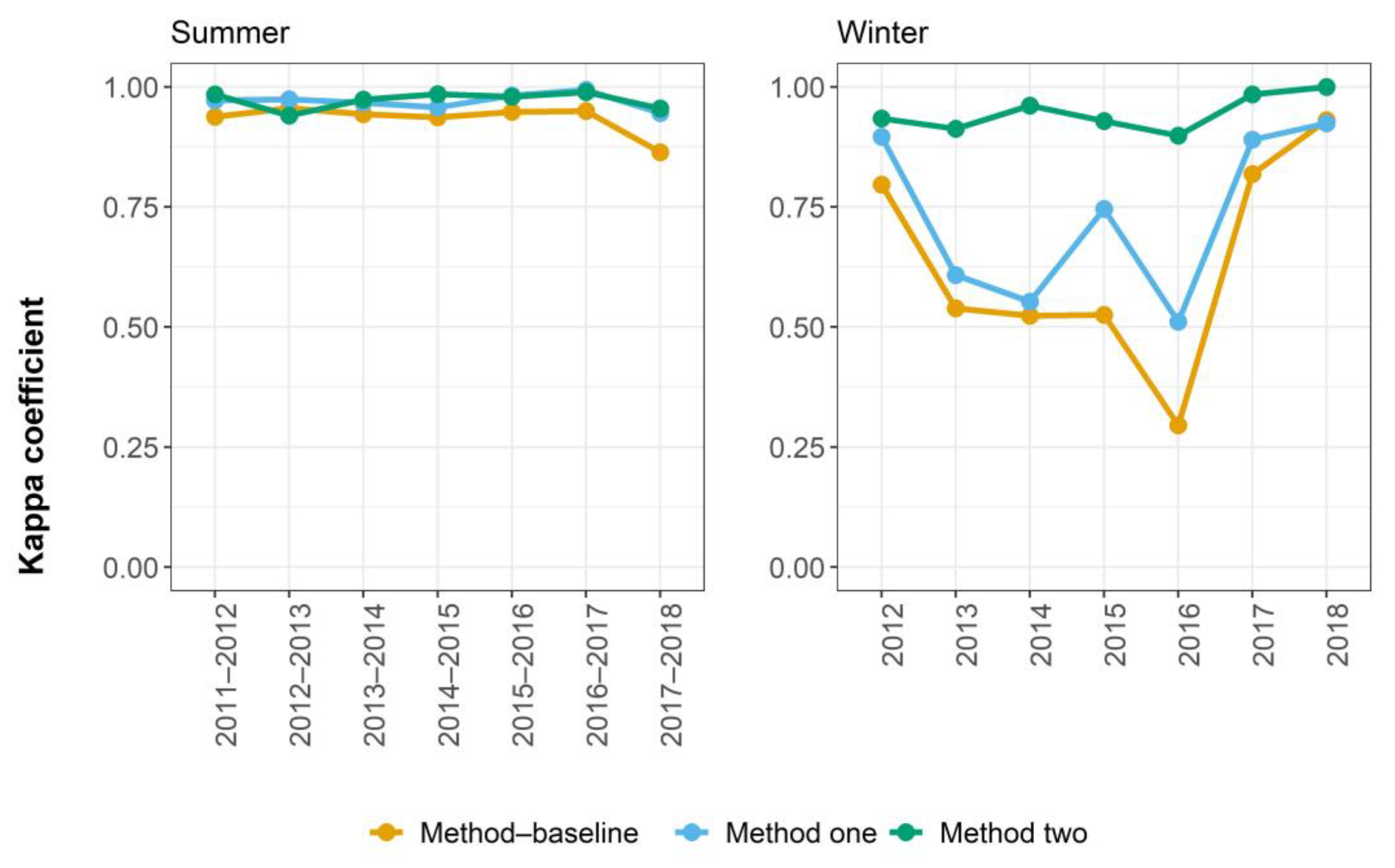
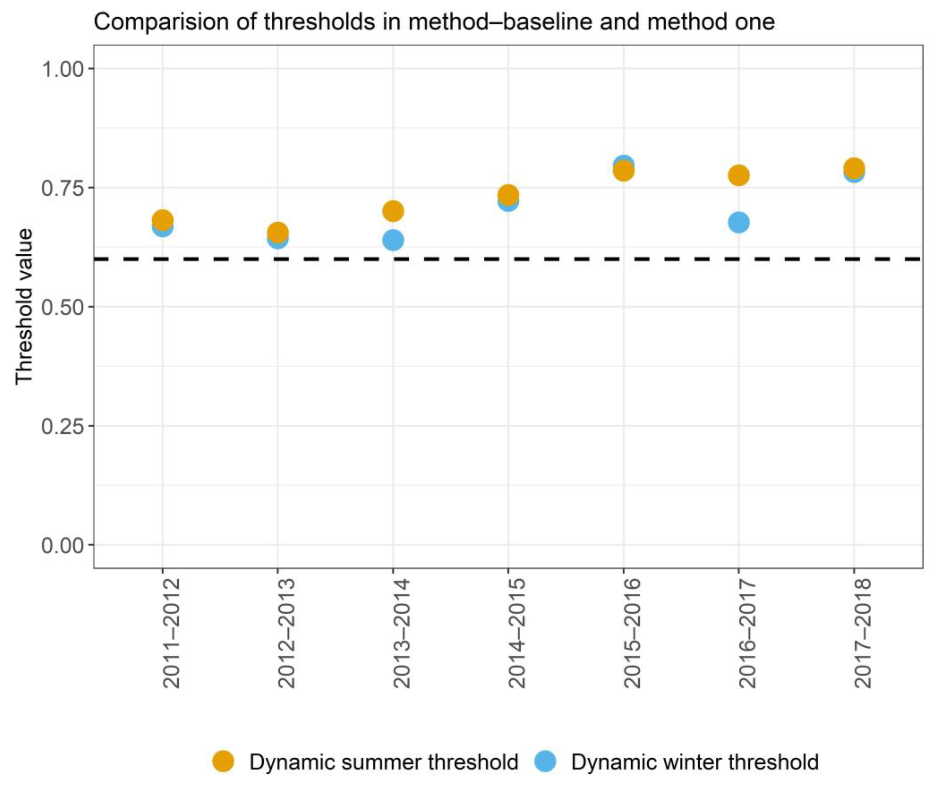
• In Section 3.1. we first compared the kappa coefficients for method one, method two and method—baseline for winter and summer classification and selected the best-performing method. A comparison between method one and method—baseline was also presented to demonstrate the importance of using dynamic thresholds.
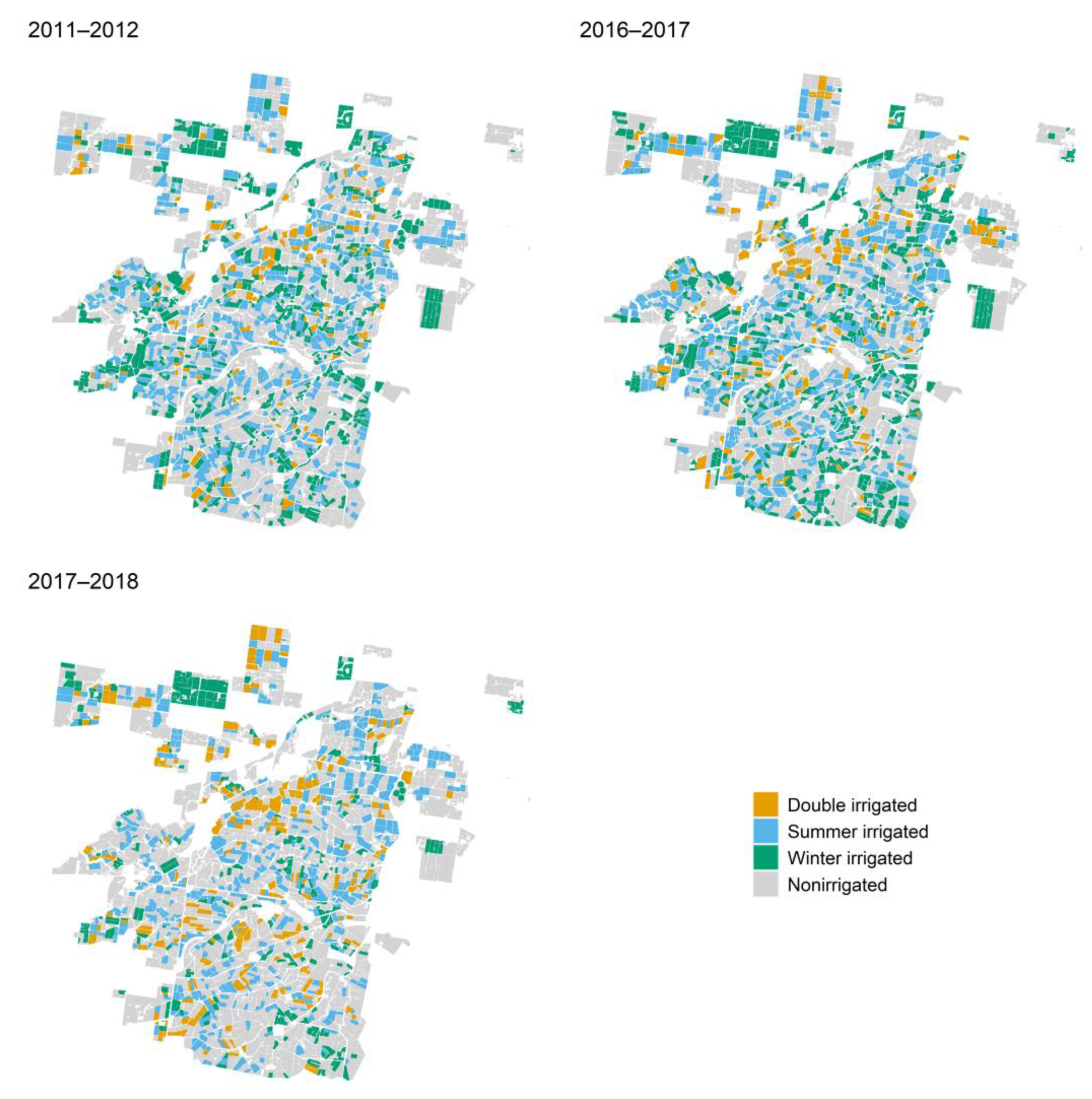
• In Section 3.2. we summarized the total classified irrigated area from the best-performing model and their comparisons with the farmer-reported areas (independent evaluation). Classified irrigated cropping maps were also presented.
• In Section 3.3. we demonstrated the improvement in classification using the GMM-based filtering method.

3.1. The Comparison of Method Performances

Figure 8 shows the validation accuracy (kappa coefficient) for the three methods in each year. We found that method two had the best accuracy, with kappa coefficients exceeding 0.9 in all tested years for both the summer and winter classifications. Method one performs well in summer, but its performance is less satisfactory in winter (i.e., 2013–2016, Figure 8). Nevertheless, method one still outperforms method—baseline for almost all years, indicating the importance of using a dynamic threshold in multiyear classification. The performance of method—baseline is limited by the static decision rules, which do not respond to different weather conditions and therefore lead to very low performance in some years (e.g., winter in 2016).

Figure 9 shows the comparison of the thresholds (MAX) used in method one and method—baseline, which suggests that the difference between the dynamic and static thresholds for both winter and summer are changing year to year. All dynamic thresholds in both seasons are larger than 0.6, suggesting the potential underestimation of the fixed threshold used in method—baseline. Furthermore, the importance of interannual variability is demonstrated by the dynamic thresholds varying over a considerable range (0.65 to 0.79 for summer and 0.64 to 0.80 for winter). This suggests that a higher static threshold would only partially address the lower performance of a static method. The detailed results for method one are shown in Figures S4 and S5 of the Supplementary Materials.

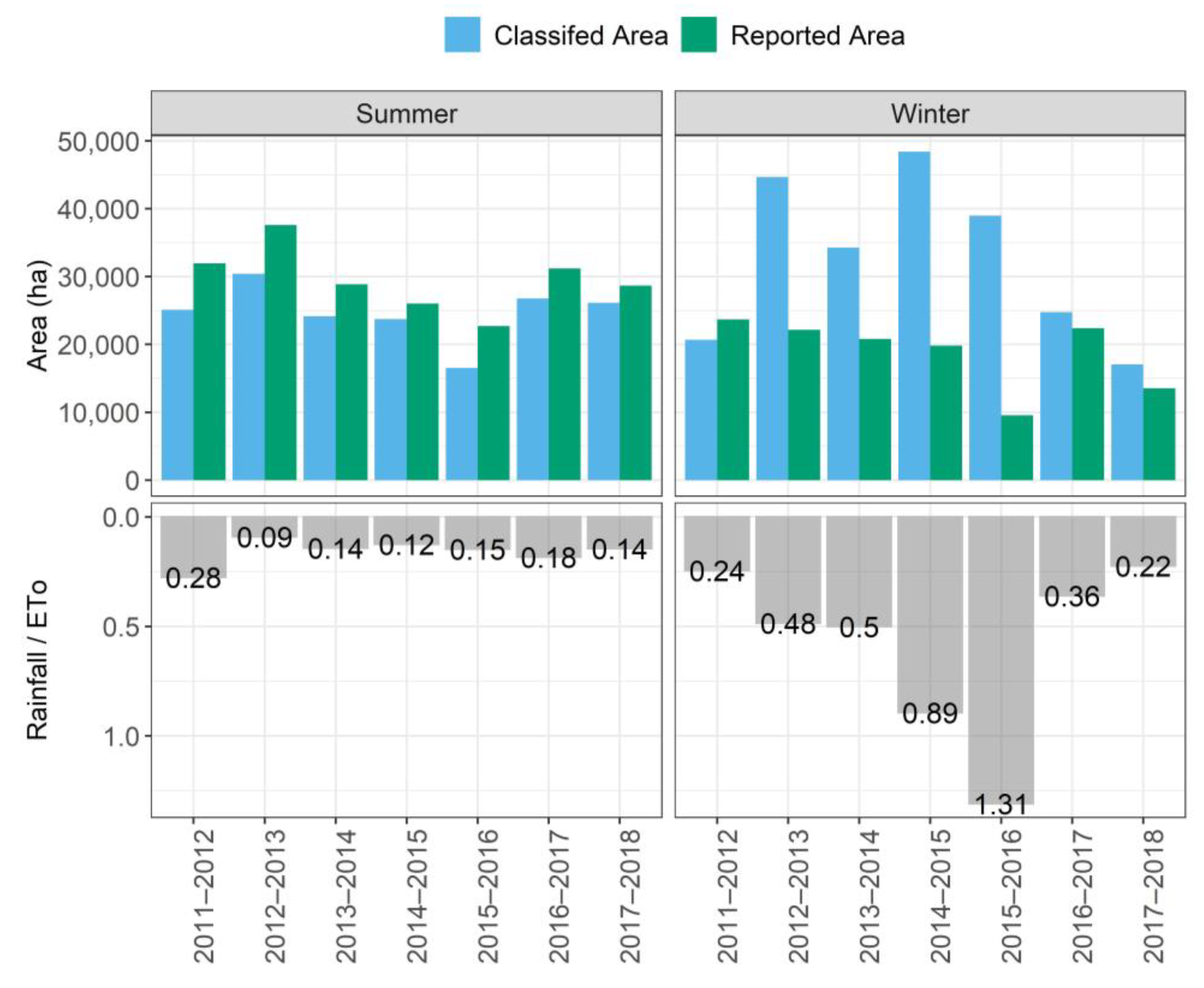
3.2. Irrigated Area Estimation Using the Best Method (Method Two) and Independent Evaluation

Method two was selected as the final method based on its consistently good performance across years and seasons. The total irrigated areas in the CIA estimated using method two across years are summarized in Figure 10, in comparison with the farmer-reported areas in the same season. The ratios of seasonal rainfall over the seasonal ETo are also shown as weather indicators. We found that when the ratio is lower than approximately 0.4 the classified and reported areas have good agreement. When the ratio is above 0.4 the discrepancy between the reported and classified areas becomes clear. This discrepancy reaches its maximum in winter 2015–16, which also has the maximum rainfall/ETo ratio of 1.31, and large numbers of rainfed cropping fields were included as irrigated in the classified maps, which reduces the accuracy of classification.

Figure 11 presents the irrigated maps for 2011–2012, 2016–2017 and 2017–2018 because these maps were considered the most reliable based on their comparison with farmer-reported areas (Figure 10). The classified maps for the remaining years are shown in Figure S6 in Section S4 of the Supplementary Materials. Overall, the summer and winter fields are scatted across the region without systematic spatial patterns of change from year to year. Besides, the locations of the summer and winter irrigated fields change from year to year.

3.3. Benefit of GMM-Based NDVI Filtering

The classification results using nonfiltered data (Target) were compared with the classification results using filtered data (Reference) to show the value of the GMM-based filtering method. The omission and commission errors are summarized in

Table 3. The commission and omission errors calculated by comparing classifications using filtered and nonfiltered data.

	Summer		Winter
Year	Omission Error	Commission Error	Omission Error	Commission Error
2011–2012	32.30%	0%	32.10%	0.20%
2012–2013	22.70%	0%	17%	0.50%
2013–2014	11.90%	0%	14.70%	0.20%
2014–2015	10%	0%	13.10%	1.10%
2015–2016	11.90%	0%	14.20%	5.10%
2016–2017	7.30%	0%	17.20%	0.50%
2017–2018	6.70%	0%	9.40%	0.30%

. We found that irrigated fields were more likely to be classified as nonirrigated fields (omission errors) using nonfiltered data. Omission error is generally higher at the start of the study period, for both summer and winter. This is most likely due to changes in field boundaries across time, indicating that the use of static field boundary layers without an innovative filtering method could lead to the loss of detection of irrigated fields. The change in field boundaries was also visualized using an example farm in two different years (Figure 12), from which we can see a clear boundary change at the left-bottom of the farm. Detailed discussions of Table 3 are presented in Section 4.1.2.

4. Discussion

4.1. Classification Methods and Recommendations

4.1.1. Selection of Classification Method

We find that the overall classification accuracy is higher for summer than winter for both method one and method two (Figure 8). Identifying irrigated areas in summer (dry season) in this semiarid region is relatively easy, as high evaporative demand combined with somewhat lower rainfall makes irrigated fields distinct from nonirrigated fields (Figure 2). This is evident in the high accuracy (kappa coefficient > 0.85, Figure 8) for all methods including method—baseline in summer, compared with kappa values often below 0.8 in winter for method one and method—baseline. Since summer is the main irrigation season, our results show a promising future for the routine monitoring of irrigated areas in the CIA using remote sensing data and classification methods. Our results suggest that summer irrigation area mapping in the CIA using any methods proposed in this study will reach good accuracy with kappa > 0.85 (Figure 8).

In contrast, identifying winter irrigated areas is more challenging, as the low ETo and high rainfall makes water no longer limited (Figure 2). In this case, simply relying on one or two key features, such as the peak seasonal NDVI used in thresholding methods, is not sufficient to differentiate the irrigated fields with nonirrigated grazing lands and forests. For example, the seasonal peak NDVI for nonirrigated grazing land in winter 2016 reached 0.7–0.8 (Figure 6), which is similar to irrigated fields. We therefore need to use multiple metrics from the time series of NDVI data to capture the minor differences between irrigated and nonirrigated fields. A sophisticated model, such as random forest, is more capable of handling large numbers of inputs than simple threshold-based decision tree models in this case. More importantly, we develop an innovative training sample pool for method two that allows for the classification rules to be automatically updated season-by-season, leading to much more consistent performance in multiyear classification, as opposed to method one, which shows relatively low performances in the winters of 2013–2016 (Figure 8).

Comparing the two thresholding methods, we find that the accuracy for method one is generally higher than for method—baseline (Figure 8). While both rely on thresholds to make decisions, the improved performance in method one comes from the implementation of the dynamic threshold. When field conditions, such as the peak season NDVI, change in response to interannual weather variability, the threshold changes correspondingly. For example, a higher threshold is given in wet winters (2016) compared to that in dry winters (2013) (Figure 2 and Figure 9). In this study, all dynamic thresholds for both summer and winter are higher than the static value of 0.6 used in method—baseline (Figure 9). With an underestimated threshold, method—baseline can misclassify some nonirrigated fields as irrigated, thus leading to overestimates of irrigated areas and lower accuracies. The improvement of method one compared to method—baseline indicates the importance of using a dynamic threshold in the classification method to support multiyear irrigated mapping. This is particularly important if the study region has large interannual variability in weather.

To summarize, method two is the most appropriate classification method for both wet and dry seasons, while method one is more appliable for the dry season but still under-performs compared with method two. Method one has a simple model structure with fewer input requirements and no requirement for training samples; however, it is less accurate in winter due to its simple model structure, which fails to distinguish the differences between nonirrigated and irrigated fields. In contrast, method two uses advanced machine learning techniques, which shows better classification performance in complex situations. Nevertheless, the performance of method two should not be exaggerated, as our independent evaluation indicates that some rainfed cropping fields may still be misclassified into irrigated fields in wet winters (high rainfall/ETo ratio, Figure 10). This is because rainfed and irrigated fields exhibit highly similar land features when water stress is low, making classification challenging.

4.1.2. Improvement in Classification Results with GMM-Based Filtered Data

By comparing the classification results predicted by method two using GMM-filtered and nonfiltered data, we conclude that the GMM-based filtering method can effectively reduce omission errors for irrigated cropping fields (Table 3). These errors are attributed to the difference in field-scale data quality. When noncrop pixels are included in pixel-to-field aggregation the NDVI profiles for cropping fields are distorted, leading to less detection of cropping fields and the underestimation of cropping areas. The maximum omission error is 32.3% (Table 3), indicating that up to approximately 1/3 of irrigated fields could be missed with nonfiltered data. Interestingly, we find smaller omission errors when the tested year is closer to the year that field boundaries were delineated (i.e., field boundaries were delineated in 2019 and omission errors follow a generally increasing trend back to 2011, Table 3). This probably indicates the impact of changing field boundaries across time (Figure 12) on classification. This error trend also indicates that the assumption of static field boundaries may not be reliable, and that the frequent updating of satellite images and field delineation is required. However, the costs of boundary delineation should also be taken into account as the delineation process requires costly very-high-resolution satellite images. Based on the results from this study, we consider regular updates of field boundary as necessary for long-term analysis. At the same time, GMM-based filtering is an effective filtering method that can improve field-level data quality and improve the quality of the classification outputs.

4.2. Multiyear Irrigated Area Monitoring and Water Management

Overall, the annual summer irrigated area in the CIA is relatively stable compared with the winter irrigated area (Figure 10). The is probably because summer and winter irrigations are subject to different controlling factors. Since the CIA has a hot and dry summer, rainfall plays a smaller role to compensate for crop evapotranspiration; summer crops rely mainly on irrigation. In this case, the total irrigation area in the district is determined by the district-level water allocation in that particular year. If water allocation is maintained at a medium-to-high level, a change in the annual irrigation area is expected to be small. When water availability is low summer irrigation areas reduce markedly, as observed in the 2015–2016 summer, which is the lowest water allocation year in the study period (37%) [53]. In contrast, winter irrigation areas are more uncertain as they are determined by both rainfall and water allocation. If rainfall is high the amount of irrigation is reduced to a small proportion to act as a supplementary to support crop growth, and if water allocations are low (and thus water prices high) winter irrigation cropping is less viable. Due to the mixture of water sources that are dominated by rainfall, winter irrigated areas change dramatically across years and are less predictable than summer irrigation areas (Figure 10).

The variation in irrigated areas across years in the CIA also highlights the importance of routine irrigation area monitoring in irrigation districts. The extent and locations of irrigated fields change very dynamically from year to year, under the influence of complex factors such as water availability, short-term weather conditions, commodity prices, long-term climate changes and changing management practices [7,8,28]. Currently, irrigation area monitoring systems are lacking in many irrigation districts, not to mention the availability of continuous and consistent high-resolution irrigated area maps [2,8]. Many parts of the world still rely on static mapping of irrigated areas. The utilization of such static maps may lead to unreliable analyses of water and food security management, irrigation performance, irrigation allocation estimates and crop yield prediction.

Remote-sensing-based classification provides a good tool to support multiyear irrigated area monitoring. However, one difficulty is that the phenology of some plants changes with annual weather, which makes a well-calibrated classification model inaccurate when transferred across years [6]. Conversely, recalibrating or redeveloping models for individual years is time-consuming and impractical. This paper provides two temporally dynamic methods to fill this gap. Method one is an unsupervised method that utilizes a statistical summary of NDVI indices of all fields and generates a dynamic threshold to better separate irrigated and nonirrigated fields in different years. Method two improves its multiyear performance by using innovative combinations of training samples that allow its classification rules to be automatically updated every year. Once trained for a district, both models are fully automatic and computationally efficient. The approaches to method development used here are highly transferable to other districts and to support long-term irrigated area monitoring.

4.3. Study Limitation

We found the performance of method two in wet winters to be less reliable due to the high vegetation cover on rainfed cropping fields. Future work could focus on establishing a separate rainfed cropping class and involving more features than NDVI and NDVI metrics that better capture the differences between rainfed and irrigated cropping fields. Another limit relates to perennial crops, which have different seasonal NDVI profiles to annual irrigated crops. These crops may be classified into the “perennial” or “unknown” classes in method two, which were further marked as nonirrigated fields. Nevertheless, perennial crops can be either rainfed or irrigated, but we lack ground samples in this study to explicitly identify perennial crops. Despite the fact that perennial crops are not common in the CIA, future studies could collect more information on ground samples of perennial crops to obtain more complete classification classes in method two, which may further improve classification results.

5. Conclusions

This paper focuses on developing field-scale data processing methods and temporally transferable classification methods to support multiyear irrigated area mapping. We solved two questions arising from current limitations in irrigated area mapping: (1) how to reduce the impact of within-field noise when converting pixel-level satellite data to the field-level, and (2) how to develop classification models that can support multiyear irrigated area classification with good accuracy by adapting between years. Key conclusions are summarized as follows:

(1) The Gaussian mixture model (GMM)-based filtering method developed in this study can automatically reduce within-field noises in individual fields, which reduces misclassification errors by up to 1/3 for both summer and winter seasons.

(2) Two temporally dynamic methods based on field-level NDVI metrics proved to be efficient in multiyear irrigated field classification. The random forest method (method two) consistently demonstrated the best performance (kappa > 0.9 in validation) for both summer and winter seasons in the study period (2011–2018), although classification errors increase in wet winters (ratio of seasonal rainfall over the seasonal ETo > 0.4).

6. Patents

This study is part of a patent that has already been filed (application No. 2021904049).

References

1. Aleksandrova, M.; Lamers, J.P.; Martius, C.; Tischbein, B. Rural vulnerability to environmental change in the irrigated lowlands of Central Asia and options for policy-makers: A review. Environ. Sci. Policy 2014, 41, 77–88. [Google Scholar] [CrossRef]
2. McAllister, A.; Whitfield, D.; Abuzar, M. Mapping irrigated farmlands using vegetation and thermal thresholds derived from Landsat and ASTER data in an irrigation district of Australia. Photogramm. Eng. Remote Sens. 2015, 81, 229–238. [Google Scholar] [CrossRef]
3. Alexandratos, N.; Bruinsma, J. World Agriculture towards 2030/2050, The 2012 Revision; Food and Agriculture Organization of the United Nations: Rome, Italy, 2012. [Google Scholar] [CrossRef]
4. Biggs, T.W.; Thenkabail, P.S.; Gumma, M.K.; Scott, C.A.; Parthasaradhi, G.R.; Turral, H.N. Irrigated area mapping in heterogeneous landscapes with MODIS time series, ground truth and census data, Krishna Basin, India. Int. J. Remote Sens. 2006, 27, 4245–4266. [Google Scholar] [CrossRef]
5. Deines, J.M.; Kendall, A.D.; Hyndman, D.W. Annual irrigation dynamics in the US Northern High Plains derived from Landsat satellite data. Geophys. Res. Lett. 2017, 44, 9350–9360. [Google Scholar] [CrossRef]
6. Ozdogan, M.; Yang, Y.; Allez, G.; Cervantes, C. Remote sensing of irrigated agriculture: Opportunities and challenges. Remote Sens. 2010, 2, 2274–2304. [Google Scholar] [CrossRef] [Green Version]
7. Pervez, M.S.; Budde, M.; Rowland, J. Mapping irrigated areas in Afghanistan over the past decade using MODIS NDVI. Remote Sens. Environ. 2014, 149, 155–165. [Google Scholar] [CrossRef] [Green Version]
8. Deines, J.M.; Kendall, A.D.; Crowley, M.A.; Rapp, J.; Cardille, J.A.; Hyndman, D.W. Mapping three decades of annual irrigation across the US High Plains Aquifer using Landsat and Google Earth Engine. Remote Sens. Environ. 2019, 233, 111400. [Google Scholar] [CrossRef]
9. Bazzi, H.; Baghdadi, N.; Ienco, D.; El Hajj, M.; Zribi, M.; Belhouchette, H.; Escorihuela, M.J.; Demarez, V. Mapping irrigated areas using Sentinel-1 Time series in Catalonia, Spain. Remote Sens. 2019, 11, 1836. [Google Scholar] [CrossRef] [Green Version]
10. Gao, Q.; Zribi, M.; Escorihuela, M.J.; Baghdadi, N.; Segui, P.Q. Irrigation mapping using Sentinel-1 time series at field scale. Remote Sens. 2018, 10, 1495. [Google Scholar] [CrossRef] [Green Version]
11. Bousbih, S.; Zribi, M.; El Hajj, M.; Baghdadi, N.; Lili-Chabaane, Z.; Gao, Q.; Fanise, P. Soil moisture and irrigation mapping in A semi-arid region, based on the synergetic use of Sentinel-1 and Sentinel-2 data. Remote Sens. 2018, 10, 1953. [Google Scholar] [CrossRef] [Green Version]
12. Holben, B.; Fraser, R.S. Red and near-infrared sensor response to off-nadiir viewing. Int. J. Remote Sens. 1984, 5, 145–160. [Google Scholar] [CrossRef]
13. Massey, R.; Sankey, T.T.; Congalton, R.G.; Yadav, K.; Thenkabail, P.S.; Ozdogan, M.; Meador, A.J.S. MODIS phenology-derived, multi-year distribution of conterminous US crop types. Remote Sens. Environ. 2017, 198, 490–503. [Google Scholar] [CrossRef]
14. Saadi, S.; Simonneaux, V.; Boulet, G.; Raimbault, B.; Mougenot, B.; Fanise, P.; Ayari, H.; Lili-Chabaane, Z. Monitoring irrigation consumption using high resolution NDVI image time series: Calibration and validation in the Kairouan Plain (Tunisia). Remote Sens. 2015, 7, 13005–13028. [Google Scholar] [CrossRef] [Green Version]
15. Zheng, B.; Myint, S.W.; Thenkabail, P.S.; Aggarwal, R.M. A support vector machine to identify irrigated crop types using time-series Landsat NDVI data. Int. J. Appl. Earth Obs. Geoinf. 2015, 34, 103–112. [Google Scholar] [CrossRef]
16. Esch, T.; Metz, A.; Marconcini, M.; Keil, M. Combined use of multi-seasonal high and medium resolution satellite imagery for parcel-related mapping of cropland and grassland. Int. J. Appl. Earth Obs. Geoinf. 2014, 28, 230–237. [Google Scholar] [CrossRef]
17. Watkins, B.; Van Niekerk, A. A comparison of object-based image analysis approaches for field boundary delineation using multi-temporal Sentinel-2 imagery. Comput. Electron. Agric. 2019, 158, 294–302. [Google Scholar] [CrossRef]
18. Chen, G.; Weng, Q.; Hay, G.J.; He, Y. Geographic Object-based Image Analysis (GEOBIA): Emerging trends and future opportunities. GISci. Remote Sens. 2018, 55, 159–182. [Google Scholar] [CrossRef]
19. Hossain, M.D.; Chen, D. Segmentation for Object-Based Image Analysis (OBIA): A review of algorithms and challenges from remote sensing perspective. ISPRS J. Photogramm. Remote Sens. 2019, 150, 115–134. [Google Scholar] [CrossRef]
20. Asgarian, A.; Soffianian, A.; Pourmanafi, S. Crop type mapping in a highly fragmented and heterogeneous agricultural landscape: A case of central Iran using multi-temporal Landsat 8 imagery. Comput. Electron. Agric. 2016, 127, 531–540. [Google Scholar] [CrossRef]
21. Debats, S.R.; Luo, D.; Estes, L.D.; Fuchs, T.J.; Caylor, K.K. A generalized computer vision approach to mapping crop fields in heterogeneous agricultural landscapes. Remote Sens. Environ. 2016, 179, 210–221. [Google Scholar] [CrossRef] [Green Version]
22. Wu, B.; Li, Q. Crop planting and type proportion method for crop acreage estimation of complex agricultural landscapes. Int. J. Appl. Earth Obs. Geoinf. 2012, 16, 101–112. [Google Scholar] [CrossRef]
23. Conrad, C.; Fritsch, S.; Zeidler, J.; Rücker, G.; Dech, S. Per-field irrigated crop classification in arid Central Asia using SPOT and ASTER data. Remote Sens. 2010, 2, 1035–1056. [Google Scholar] [CrossRef] [Green Version]
24. Cai, Y.; Guan, K.; Peng, J.; Wang, S.; Seifert, C.; Wardlow, B.; Li, Z. A high-performance and in-season classification system of field-level crop types using time-series Landsat data and a machine learning approach. Remote Sens. Environ. 2018, 210, 35–47. [Google Scholar] [CrossRef]
25. De Castro, A.I.; Six, J.; Plant, R.E.; Peña, J.M. Mapping crop calendar events and phenology-related metrics at the parcel level by object-based image analysis (OBIA) of MODIS-NDVI time-series: A case study in central California. Remote Sens. 2018, 10, 1745. [Google Scholar] [CrossRef] [Green Version]
26. Park, S.; Ryu, D.; Fuentes, S.; Chung, H.; Hernández-Montes, E.; O’Connell, M. Adaptive estimation of crop water stress in nectarine and peach orchards using high-resolution imagery from an unmanned aerial vehicle (UAV). Remote Sens. 2017, 9, 828. [Google Scholar] [CrossRef] [Green Version]
27. Zhong, L.; Gong, P.; Biging, G.S. Efficient corn and soybean mapping with temporal extendability: A multi-year experiment using Landsat imagery. Remote Sens. Environ. 2014, 140, 1–13. [Google Scholar] [CrossRef]
28. Ambika, A.K.; Wardlow, B.; Mishra, V. Remotely sensed high resolution irrigated area mapping in India for 2000 to 2015. Sci. Data 2016, 3, 160118. [Google Scholar] [CrossRef] [Green Version]
29. Brief Overview of CICL. Available online: https://www.colyirr.com.au/brief-overview (accessed on 4 January 2022).
30. Annual Compliance Report; Coleambally Irrigation Co-Operative Limited (CICL): Coleambally, NSW, Australia, 2020; p. 23. Available online: https://static1.squarespace.com/static/5af3b1ae70e8023a6ac7a10b/t/5b04dca38a922da81bbf74c8/1527045455569/ACR+2016.pdf (accessed on 20 December 2021).
31. Evapotranspiration Calculations. Available online: http://www.bom.gov.au/watl/eto/tables/nsw/narrabri_airport/narrabri_airport.shtml (accessed on 4 December 2021).
32. Jackson, T.M.; Khan, S.; Hafeez, M. A comparative analysis of water application and energy consumption at the irrigated field level. Agric. Water Manag. 2010, 97, 1477–1485. [Google Scholar] [CrossRef]
33. Education and Research Program. Available online: https://www.planet.com/markets/education-and-research/ (accessed on 15 January 2020).
34. Gorelick, N.; Hancher, M.; Dixon, M.; Ilyushchenko, S.; Thau, D.; Moore, R. Google Earth Engine: Planetary-scale geospatial analysis for everyone. Remote Sens. Environ. 2017, 202, 18–27. [Google Scholar] [CrossRef]
35. Blaschke, T. Object based image analysis for remote sensing. ISPRS J. Photogramm. Remote Sens. 2010, 65, 2–16. [Google Scholar] [CrossRef] [Green Version]
36. Laliberte, A.; Rango, A.; Herrick, J.; Fredrickson, E.L.; Burkett, L. An object-based image analysis approach for determining fractional cover of senescent and green vegetation with digital plot photography. J. Arid Environ. 2007, 69, 1–14. [Google Scholar] [CrossRef]
37. Ryherd, S.; Woodcock, C. Combining spectral and texture data in the segmentation of remotely sensed images. Photogramm. Eng. Remote Sens. 1996, 62, 181–194. [Google Scholar]
38. Extract Segments Only. Available online: https://www.l3harrisgeospatial.com/docs/segmentonly.html (accessed on 4 January 2022).
39. Jin, X. Segmentation-Based Image Processing System. U.S. Patent US20090123070A1, 14 May 2009. [Google Scholar]
40. Xu, L.; Ming, D.; Zhou, W.; Bao, H.; Chen, Y.; Ling, X. Farmland Extraction from High Spatial Resolution Remote Sensing Images Based on Stratified Scale Pre-Estimation. Remote Sens. 2019, 11, 108. [Google Scholar] [CrossRef] [Green Version]
41. Carlson, T.N.; Gillies, R.R.; Perry, E.M. A method to make use of thermal infrared temperature and NDVI measurements to infer surface soil water content and fractional vegetation cover. Remote Sens. Rev. 1994, 9, 161–173. [Google Scholar] [CrossRef]
42. Ozelkan, E.; Chen, G.; Ustundag, B.B. Multiscale object-based drought monitoring and comparison in rainfed and irrigated agriculture from Landsat 8 OLI imagery. Int. J. Appl. Earth Obs. Geoinf. 2016, 44, 159–170. [Google Scholar] [CrossRef]
43. Tucker, C.J. Red and photographic infrared linear combinations for monitoring vegetation. Remote Sens. Environ. 1979, 8, 127–150. [Google Scholar] [CrossRef] [Green Version]
44. Sayler, K. Landsat 8 Collection 1 (C1) Land Surface Reflectance Code (LaSRC) Product Guide. Available online: https://prd-wret.s3.us-west-2.amazonaws.com/assets/palladium/production/atoms/files/LSDS-1368_L8_C1-LandSurfaceReflectanceCode-LASRC_ProductGuide-v3.pdf (accessed on 12 December 2021).
45. Zeng, L.; Wardlow, B.D.; Xiang, D.; Hu, S.; Li, D. A review of vegetation phenological metrics extraction using time-series, multispectral satellite data. Remote Sens. Environ. 2020, 237, 111511. [Google Scholar] [CrossRef]
46. Fraley, C.; Raftery, A.E.; Murphy, T.B.; Scrucca, L. Mclust Version 4 for R: Normal Mixture Modeling for Model-Based Clustering, Classification, and Density Estimation; Technical Report 597; Department of Statistics, University of Washington: Seattle, WA, USA, 2012. [Google Scholar]
47. Senturk, S.; Bagis, S.; Ustundag, B.B. Application of remote sensing techniques in locating dry and irrigated farmland parcels. In Proceedings of the 2014 the Third International Conference on Agro-Geoinformatics, Beijing, China, 11–14 August 2014; pp. 1–4. [Google Scholar]
48. Rodriguez-Galiano, V.F.; Ghimire, B.; Rogan, J.; Chica-Olmo, M.; Rigol-Sanchez, J.P.; Sensing, R. An assessment of the effectiveness of a random forest classifier for land-cover classification. ISPRS J. Photogramm. Remote Sens. 2012, 67, 93–104. [Google Scholar] [CrossRef]
49. Lebourgeois, V.; Dupuy, S.; Vintrou, É.; Ameline, M.; Butler, S.; Bégué, A. A combined random forest and OBIA classification scheme for mapping smallholder agriculture at different nomenclature levels using multisource data (simulated Sentinel-2 time series, VHRS and DEM). Remote Sens. 2017, 9, 259. [Google Scholar] [CrossRef] [Green Version]
50. RColorBrewer, S.; Liaw, M.A. Package ‘randomForest’; University of California, Berkeley: Berkeley, CA, USA, 2018. [Google Scholar]
51. Konduri, V.S.; Kumar, J.; Hargrove, W.W.; Hoffman, F.M.; Ganguly, A.R. Mapping crops within the growing season across the United States. Remote Sens. Environ. 2020, 251, 112048. [Google Scholar] [CrossRef]
52. Peña-Arancibia, J.L.; McVicar, T.R.; Paydar, Z.; Li, L.; Guerschman, J.P.; Donohue, R.J.; Dutta, D.; Podger, G.M.; van Dijk, A.I.; Chiew, F.H. Dynamic identification of summer cropping irrigated areas in a large basin experiencing extreme climatic variability. Remote Sens. Environ. 2014, 154, 139–152. [Google Scholar] [CrossRef]
53. Annual Compliance Report; Coleambally Irrigation Co-Operative Limited (CICL): Coleambally, NSW, Australia, 2016; p. 4. Available online: https://static1.squarespace.com/static/5af3b1ae70e8023a6ac7a10b/t/5b04dca38a922da81bbf74c8/1527045455569/ACR+2016.pdf (accessed on 20 December 2021).
Figure 1. The study area—Coleambally Irrigation Area (CIA). The background image comes from the true-color Landsat composite obtained in summer 2013–2014. The inserted map at the bottom-right corner shows the location of the CIA in Australia.
Remotesensing 14 00997 g001
Figure 2. Summer and winter rainfall as well as the ETo from 2011 to 2018 in the CIA. The summer ETo and rainfall were the accumulation of the daily ETo and rainfall from October to March, respectively, and the winter ETo and rainfall were the accumulation of the daily ETo and rainfall from April to September, respectively.
Remotesensing 14 00997 g002
Figure 3. The flow diagram of the methodology. Section 2.4.1, Section 2.4.2, Section 2.5.1, Section 2.5.2, Section 2.5.4, Section 2.5.5 and Section 6.
Remotesensing 14 00997 g003
Figure 4. The flowchart of the GMM-based filtering method. (a) Field conditions; (b) applying 2-component GMM on NDVI values; (c) the GMM decision tree; and (d) final results (the representative pixels were shown with black dots).
Remotesensing 14 00997 g004
Figure 5. The decision tree for method one.
Remotesensing 14 00997 g005
Figure 6. (A) Examples of static fields in winter; (B) examples of static fields in summer; (C) nonirrigated grazing land samples collected via Google Earth; and (D) forest samples collected via Google Earth. Images for nonirrigated grazing land and forests from Google Earth are displayed in Section S3 of the Supplementary Materials (Figure S3).
Remotesensing 14 00997 g006
Figure 7. Training samples for winter and summer classification. Each point represents a field. The nonirrigated grazing samples were collected at the surrounding area of the CIA.
Remotesensing 14 00997 g007
Figure 8. Method validation accuracies for winter and summer irrigated field classification, respectively.
Remotesensing 14 00997 g008
Figure 9. The comparison of the threshold (MAX) used in method—baseline and method one. The black, dashed line indicates the fixed value of the MAX (0.6) used in method—baseline.
Remotesensing 14 00997 g009
Figure 10. The classified irrigated areas (unit: ha) and their comparisons with the farmer-reported areas. The ratio of rainfall over the ETo was presented as a weather indicator, showing the crop water availability and irrigation requirement in each season.
Remotesensing 14 00997 g010
Figure 11. The irrigated area maps for 2011–2012, 2016–2017 and 2017–2018. The class “Double irrigated” represents fields that are classified as both summer and winter irrigated fields in one cropping year.
Remotesensing 14 00997 g011
Figure 12. The change in field boundaries shown by Landsat 8 false-color composite (band 5-4-3) in an example farm in two different years.
Remotesensing 14 00997 g012