Article

Can Multi-Mission Altimeter Datasets Accurately Measure Long-Term Trends in Wave Height?

1
Department of Infrastructure Engineering, The University of Melbourne, Parkville, VIC 3010, Australia
2
Department of Mathematics, Faculty of Mathematics and Natural Sciences, Hasanuddin University, Makassar 90245, Indonesia
*
Author to whom correspondence should be addressed.
Remote Sens. 2022, 14(4), 974; https://doi.org/10.3390/rs14040974
Submission received: 5 January 2022 / Revised: 7 February 2022 / Accepted: 13 February 2022 / Published: 16 February 2022

Abstract

:
A long-duration, multi-mission altimeter dataset is analyzed to determine its accuracy in determining long-term trends in significant wave height. Two calibration methods are investigated: “altimeter–buoy” calibration and “altimeter–altimeter” calibration. The “altimeter–altimeter” approach shows larger positive trends globally, but both approaches are subject to temporal non-homogeneity between altimeter missions. This limits the accuracy of such datasets to approximately ±0.2 cm/year in determining trends in significant wave height. The sampling pattern of the altimeters is also investigated to determine if under-sampling impacts the ability of altimeters to measure trends for higher percentiles. It is concluded that, at the 99th percentile level, sampling issues result in a positive bias in values of trend. At lower percentiles (90th and mean), the sampling issues do not bias the trend estimates significantly.

1. Introduction

Over recent decades, significant research has focused on the temporal variability of global ocean surface wave climate. This includes studies of both long-term trends, potentially as a result of anthropogenic climate change, and the impact of multi-year atmospheric modes on the significant wave height, H s . Changes in global ocean wave climate are potentially important for a range of reasons, including engineering design and operation of vessels and facilities [1], the impacts on coastal erosion [2] and flooding [3,4], the breakup of polar sea-ice [5], and the dynamics of marine ecosystems [6].
Such studies are demanding, as they aim to identify relatively small trends or changes in multi-decadal records in the presence of large seasonal variations. Studies have used a variety of data sources, including buoy measurements, ship visual observations, microseisms, satellite altimeter measurements, and model hindcasts and projections. In situ buoy observations are the most obvious data source for such studies and have been extensively used [7,8,9,10]. Wave buoys, which measure the acceleration of the floating buoy, have been the mainstay of ocean wave monitoring for decades and are regarded as a highly reliable source of wave data. When applied to the determination of changes in wave climate, however, they have a number of limitations. Deployment at locations where there is near-continuous data for more than 25 years is still limited. Most importantly, however, differences in buoy hull types, instrumentation, and analysis methods over time mean that long-duration records from individual buoys are seldom homogeneous. The non-homogeneity manifests as discontinuities over time, which results in unacceptable bias in trend estimation [11,12,13].
By far the longest record of measurements to assess trends in significant wave height comes from Voluntary Observing Ships (VOS). Quality controlled VOS data date from the 1950s and have been extensively used to assess trends in wave height [14,15]. Despite the long temporal duration of such data, VOS observations suffer from a number of limitations, including the non-homogeneous spatial distribution of data (limited to shipping routes), bias introduced by ship size, and the nature of visual estimates. Despite careful analysis to address such issues [16], reliable estimates of relatively small values of trends are challenging from such data.
Seismic records span long durations (more than 100 years), and it is well known that interacting ocean waves generate noise signatures in such records (microseisms) [17,18,19]. Despite the obvious potential of such long duration records for the investigation of wave climate change, microseisms still represent a research field that is too immature to yield results of the accuracy required [20].
As with other fields of climate science, numerical modelling has represented a core component of wave climate research. Third generation global wave models, such as WAM and Wavewatch III [21,22], have shown an ability to model historical wave climates accurately [23,24,25]. As such, these models have been extensively used for studies of changes in wave climate over the historical period [26,27,28,29,30,31,32,33,34,35,36,37,38]. In addition, they have been forced with winds from climate models to project future changes in wave climate [39,40,41,42,43,44]. Long-duration wave model simulations fall into two categories: hindcasts, in which the model is driven by a given wind field [25,45], and reanalyzes, where they also include satellite data assimilation [23,26]. The application of reanalysis models to determine long-term trends in wave height has been questioned due to the non-homogeneity introduced with the commencement of satellite assimilation in the early 1990s [20]. However, even hindcasts are not completely free of such non-homogeneities as the wind fields which drive such hindcasts are generated by atmospheric circulation models, which include assimilated data from buoys, ship observations, and satellites. The density of these assimilated data has changed significantly over time, impacting the wind fields and hence the resulting wave conditions [46].
In order to assess the performance of models in reproducing long-term trends in wave climate, validation or ground-truth data are required. Noting the limitations of buoys, VOS, and microseismic data, satellite altimeter data have filled this need. Satellite altimeters have been in operation since the launch of GEOSAT in 1985. With the exception of the gap from 1989 to 1991, when ERS1 became operational, there has been a continuous global altimeter record from multiple satellites [47]. Altimeters relate the leading edge of the return signal from the altimeter to H s . The accurate determination of this relationship requires careful calibration against buoys, particularly if data from multiple altimeters are to be pooled to determine long-term changes in wave climate [20,47,48,49,50,51]. As a total of 14 altimeters have been operational over this period, care must be taken to ensure they are consistently calibrated and free from drift and discontinuities if they are to be used to determine long-term changes in wave climate. Two such multi-mission altimeter databases have been developed [47,51]. Ribal and Young [47] calibrated each of the altimeters independently against a large number of offshore buoys from the U.S. National Data Buoy Center (NDBC) buoy archive. We subsequently term this process “altimeter–buoy” calibration. The dataset of Dodet et al. [51] builds on the earlier GlobWave project [52], which also used “altimeter–buoy” calibration. A number of more recent missions were then added. Dodet et al. [51] adopted the GlobWave [52] “altimeter–buoy” calibrations for the earlier missions but calibrated JASON1, JASON3, CRYOSAT, and SARAL against the JASON2 altimeter at cross-over points between the satellites. We subsequently term this process of calibrating one altimeter against another mission as “altimeter–altimeter” calibration. This approach of calibrating one satellite mission against another has also been adopted to develop long-term datasets of wind speed from multi-mission radiometer data [53].
Timmermans et al. [20] determined long-term trends in mean H s and compared these trends against both the ERA5 reanalysis [24] and the CY46R1 hindcast [54]. Both altimeter datasets showed results similar to the model trends, but the Dodet et al. [51] dataset showed stronger positive trends than that of Ribal and Young [47]. Timmermans et al. [20] speculated that the differences may be a result of the different calibration processes adopted. Liu et al. [25] showed that compared to their hindcast model results, global averages of the Ribal and Young [47] altimeter data showed non-homogeneity between missions. This suggests that the “altimeter–buoy” calibration process may not produce the long-term stability desired for determining small trends in wave climate.
A further issue concerning altimeter data is the potential for under-sampling due to the orbit parameters and footprint of the altimeters. Altimeters measure over a footprint size of between 5 and 8 km in diameter. When radar returns are averaged at 1 Hz (normal period for data), they record a value of H s approximately every 8 km along the track. Altimeters are typically placed in near-polar orbits with exact repeat missions (time between orbits repeating the same ground track) between 3 and 30 days. This means that the cross-track separation between ground tracks can be hundreds of kilometers. This has raised the question of whether altimeters potentially miss the peaks of storms and hence under-sample the wave field, particularly at the extremes [20,49,50,55].
This paper aims to investigate these issues of calibration method and sampling density for long-duration, multi-mission altimeter data. Based on this analysis, the limitations of this data source can be understood when used to assess changes in global wave climate. Section 2 outlines the analysis used. The altimeter dataset used [47] is described, and two calibration methods are applied to the data, “altimeter–buoy” and “altimeter–altimeter”. The details of these calibration methods are described. In Section 3.1 and Section 3.2, global trend analysis is undertaken for both calibration methods and the differences investigated. The impacts of sampling density of altimeters on resulting trends in mean and extreme values are assessed in Section 3.3. Section 4 discusses the suitability of multi-mission altimeter data for the determination of long-term trends in significant wave height based on the analysis.

2. Materials and Methods
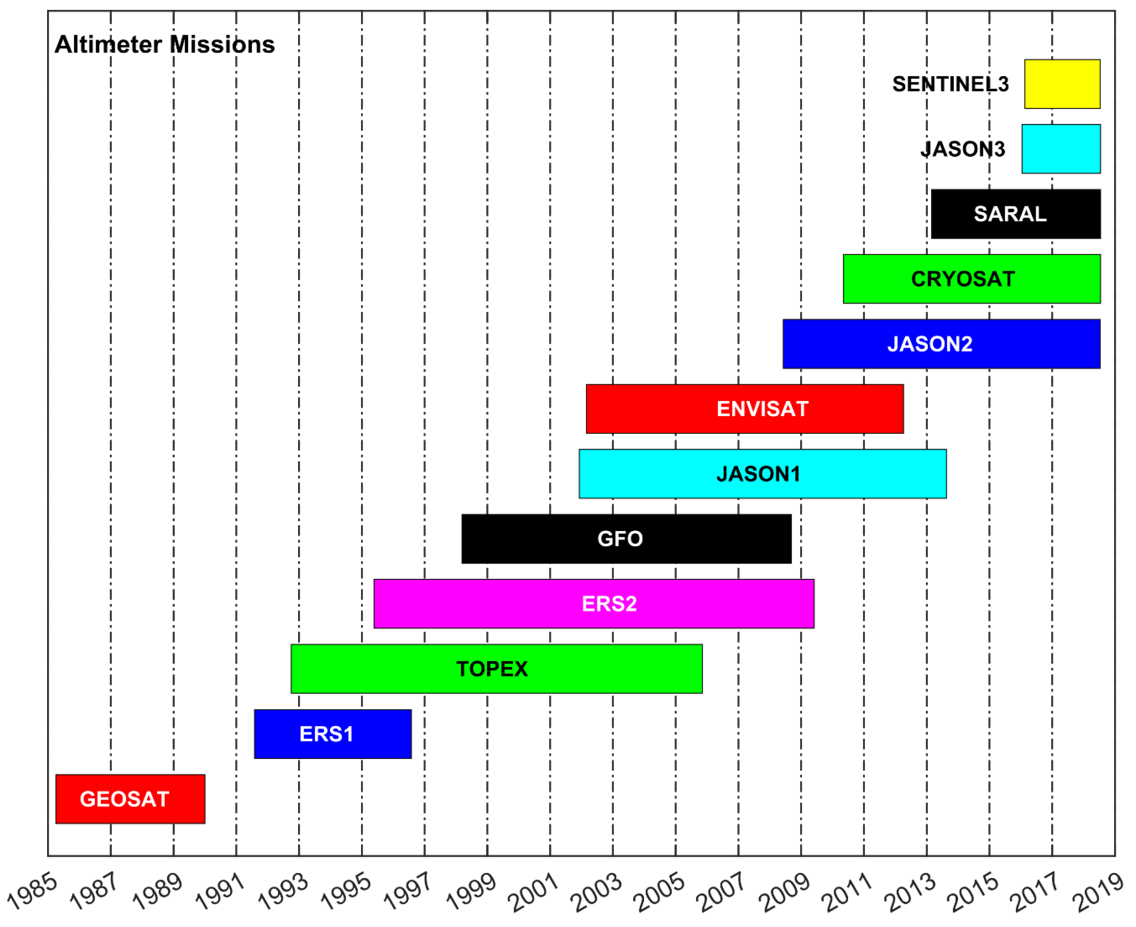
2.1. Altimeter Data

The multi-mission altimeter dataset of Ribal and Young [47], archived on the Australian Ocean Data Network (AODN) (https://portal.aodn.org.au/ (16 March 2020)), was chosen as the reference dataset for the analysis. The following 12 altimeter missions, in order of launch, were used in the analysis: GEOSAT, ERS1, TOPEX, ERS2, GFO, JASON1, ENVISAT, JASON2, CRYOSAT, SARAL, JASON3, and SENTINEL3 (note SENTINEL3 is actually SENTINEL3A but is defined in this manner as SENTINEL3B was not operational during this period). The duration of each mission is shown in Figure 1.
The AODN altimeter data records contain both the uncalibrated values of H s and the data as calibrated by Ribal and Young [47]. The 1 Hz data for both quantities from each of the altimeters above were used in the analysis below.

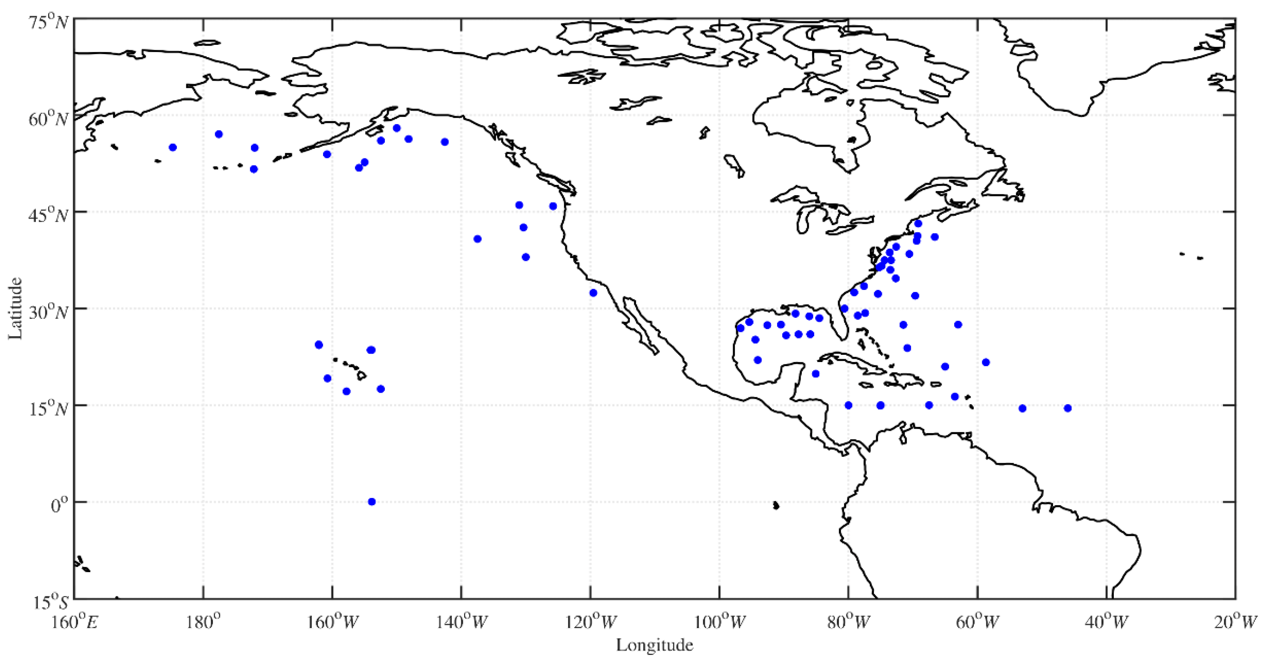
2.2. Altimeter–Buoy Calibration

Following Ribal and Young [47], a matchup between a buoy and altimeter was defined if the altimeter ground track was within 50 km of the buoy location and the time of the satellite pass was within 30 min of the buoy recording. A linear Reduced Major Axis (RMA) regression [56] was then applied to calibrate the altimeter values based on the buoy observations (“altimeter–buoy” calibration). Outliers were detected and removed before calibration using robust regression [57]. The final calibration results are given in Ribal and Young [47] (their Online Table 1). The NDBC buoy dataset was used for this calibration, with the buoy locations shown in Figure 2.

2.3. Altimeter–Altimeter Calibration

As shown in Figure 1, for the period 1991 to the present, there have been multiple altimeters in orbit at the same time. This allows comparisons to be made between these altimeters at matchup points. The same matchup criteria as used for the “altimeter–buoy” calibration were adopted: 50 km and 30 min. JASON2 was firstly calibrated against buoys. JASON1, CRYOSAT, SARAL, JASON3, and SENTINEL3 were then calibrated against JASON2 (“altimeter–altimeter” calibration). To calibrate the earlier missions which were not in operation at the same time as JASON2, the JASON1 (“altimeter–altimeter” calibration) was taken as reference and ENVISAT, GFO, and ERS2 were calibrated against JASON1. TOPEX was then calibrated against ERS2, and ERS1 was calibrated against TOPEX.
The aim of the calibration is to “correct” the raw significant wave height measurements based on the previously calibrated/corrected altimeter mission. This was undertaken using linear regression. However, both the previously calibrated altimeter and the altimeter being calibrated will contain both sampling and calibration errors [58]. As a consequence, a conventional regression analysis is not appropriate. In such cases, however, a Reduced Major Axis (RMA) regression can be used [56]. This regression minimizes the triangular area bounded by the vertical and horizontal offsets between the data point and the regression line and the cord of the regression line. This is in contrast to a conventional regression which minimizes the vertical axis offset from the regression line. In addition, standard least squares regression analysis is highly sensitive to outliers. Such outliers can be removed by the use of robust regression [57]. Robust regression assigns a weight to each point, with values between 0 and 1. Points with a value less than 0.01 were designated as outliers and removed from the analysis before applying the RMA regression analysis. The results of the RMA regression, as outlined above, for the “altimeter–altimeter” calibration for all altimeters are shown in Table A1 (Appendix A). This is the same process used for the “altimeter–buoy” calibrations [47].
As shown in Table A1, the number of matchups ranges between 1631 (SENTINEL3–JASON2) and 49,264 (JASON1–JASON2). Although matchups typically are distributed across the globe, they are concentrated at high latitudes, as shown in the examples in Figure 3.

3. Results

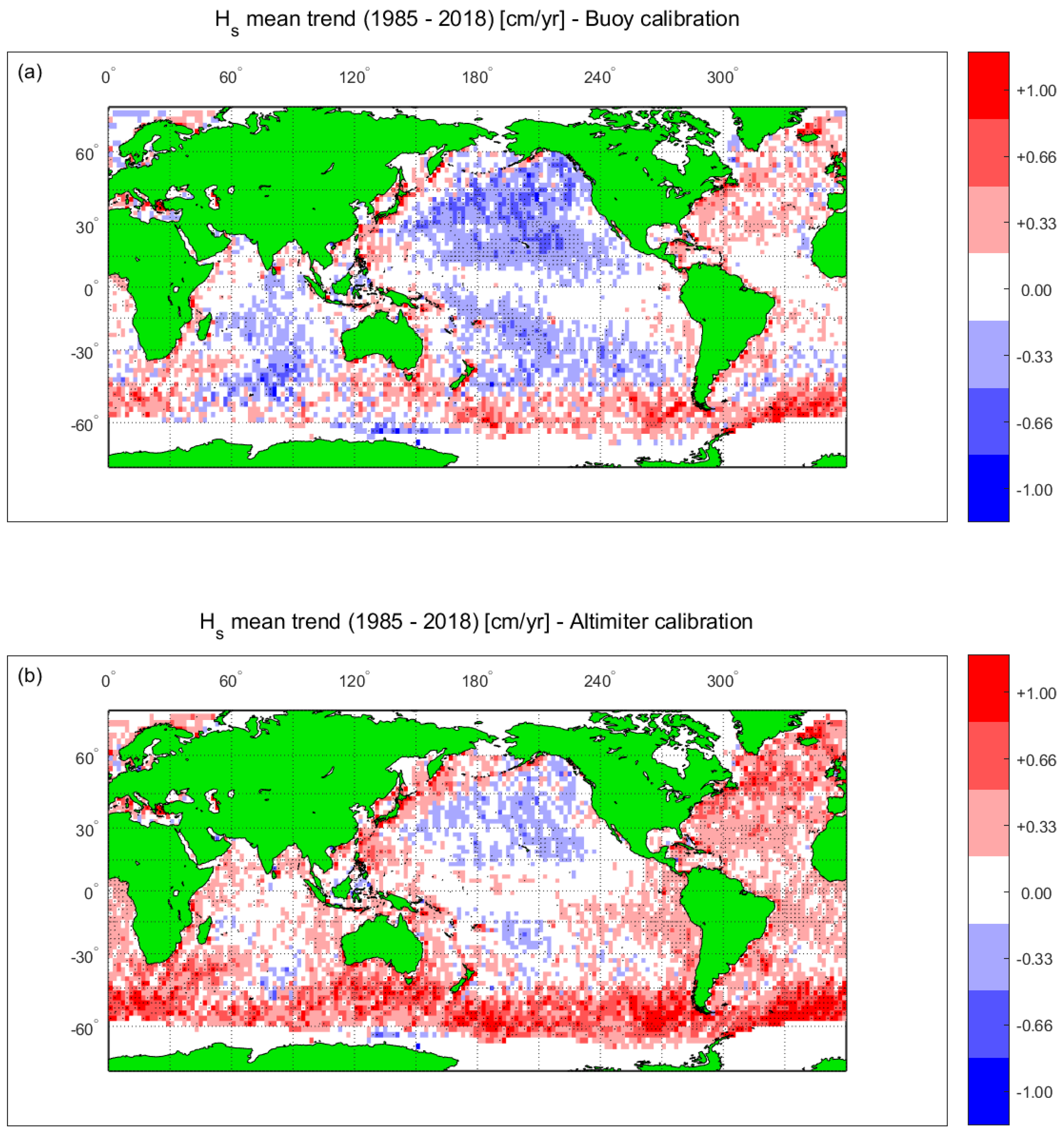
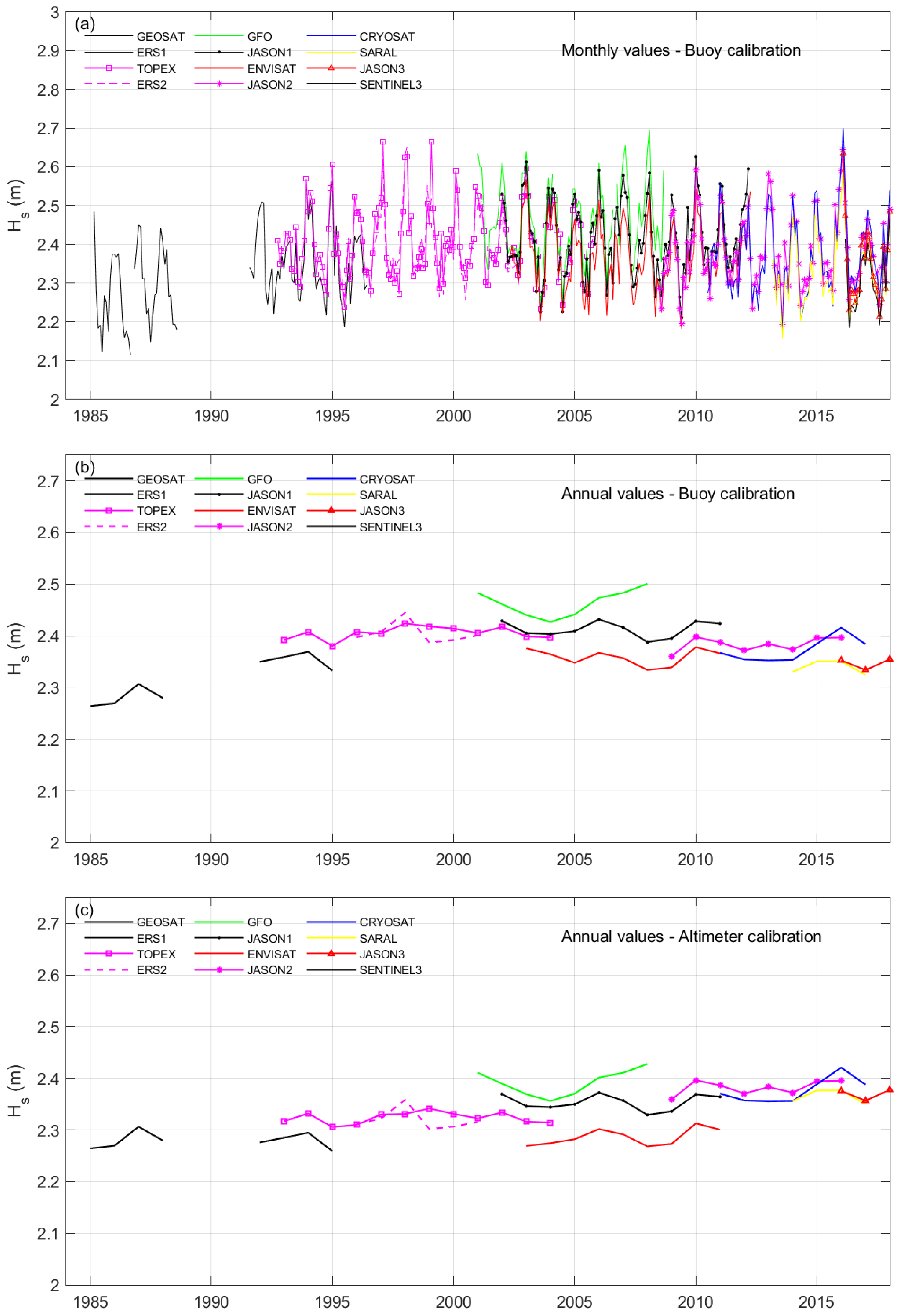
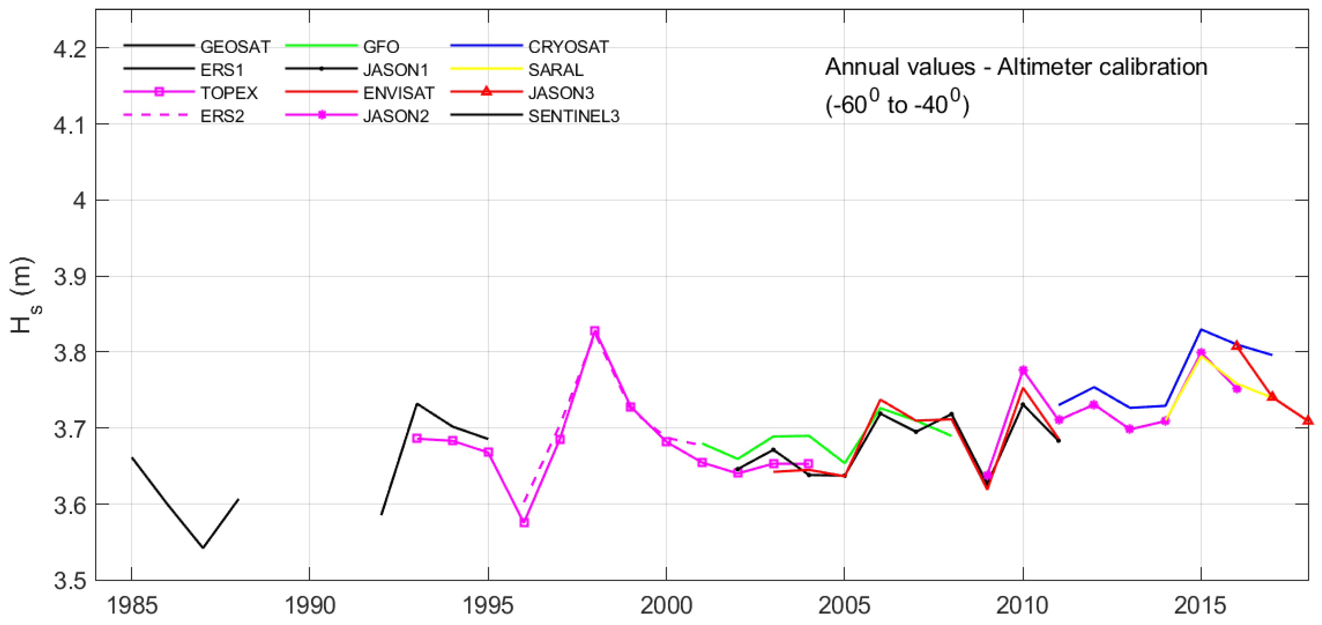
3.1. Global Trend in Mean Significant Wave Height

Following the approach of Young and Ribal [50], the data were pooled into 2° by 2° bins and mean monthly values of H s determined for each bin. The trend was then determined as the Sen slope [59,60,61]. Figure 4 shows the global distribution of trends for the “altimeter–buoy” calibration (Figure 4a) and the “altimeter–altimeter” calibration (Figure 4b). Both approaches show a band of increasing H s across the Southern Ocean. Consistent with the results of Timmermans et al. [20], the “altimeter–altimeter” calibration generally shows more positive trends than the “altimeter–buoy” calibration. The “altimeter–altimeter” calibration shows positive trends across the Southern Ocean of up to 1 cm/year. Smaller positive trends also extend across both the North and South Atlantic (0.3 cm/year). The Indian Ocean shows no clear trend, and the North Pacific shows a small negative trend (−0.3 cm/year). In contrast, the “altimeter–buoy” calibration shows a generally positive trend across the Southern Ocean of approximately 0.3 cm/year. The South Atlantic shows no clear trend, and the North Atlantic has a positive trend of less than 0.3 cm/year. The North and South Pacific show a negative trend of approximately −0.6 cm/year, and the Indian Ocean shows a negative trend of less than −0.6 cm/year. Overall, the “altimeter–buoy” calibration results are approximately 0.2 cm/year smaller than the “altimeter–altimeter” results.
Based on the results in Figure 4, it is clear that the calibration approach has impacted the values of the trend. In order to investigate how the calibration differs for each altimeter globally, mean values were determined over each altimeter mission for each 2° bin. Values of the global distributions of differences were then formed as: Δ H ¯ s = H ¯ s a l t b u o y H ¯ s a l t a l t , where H ¯ s a l t b u o y and H ¯ s a l t a l t are mean values of H s for the “altimeter–buoy” and “altimeter–altimeter” calibrations, respectively. As JASON2 was only calibrated against buoys in both approaches, it is taken as the reference, with all values being zero. Figure 5 shows the values of Δ H ¯ s for each altimeter. It is clear from this figure that for all altimeters earlier than JASON2, Δ H ¯ s is negative and for all altimeters later than JASON2, Δ H ¯ s is positive. That is, for each of the altimeters in operation after JASON2, the “altimeter–altimeter” calibration yields globally a higher wave climate than the corresponding “altimeter–buoy” calibration for that altimeter. For altimeters in operation before JASON2, the opposite occurs. Hence, it is not surprising that the “altimeter–altimeter” calibration results in a globally more positive trend (see Figure 4).
For the majority of the altimeter missions shown in Figure 5, the difference between the “altimeter–altimeter” and “altimeter–buoy” calibrations are relatively constant across the globe. However, for both CRYOSAT and SENTINEL3, there are larger differences at higher latitudes, compared to equatorial regions. The reason for this is not entirely clear and may be a subject for further research. However, it is interesting to note that these instruments are both Delay Doppler or SAR mode altimeters [62]. It may be that the calibrations of SAR-mode altimeters differ geographically compared to conventional Low-Resolution Mode (LRM) altimeters. This issue of geographic variation in calibration is explored for all altimeters in Section 3.2.

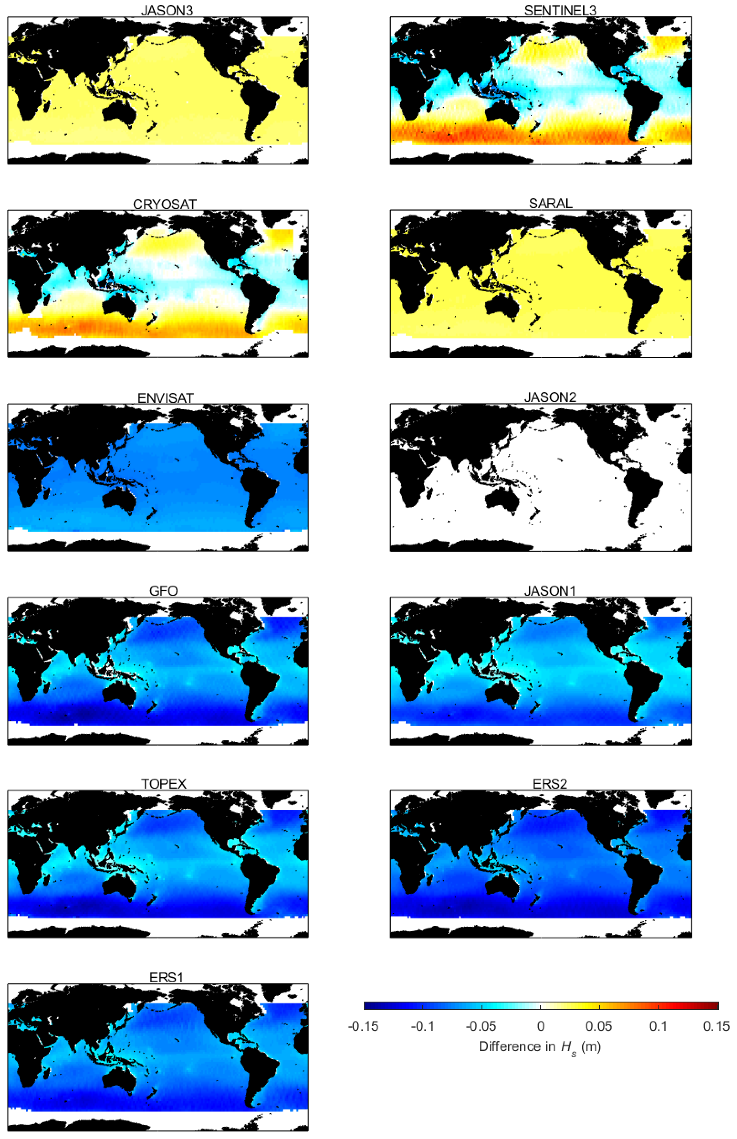
3.2. Homogeneity of Calibrated Multi-Mission Altimeter Data

As shown by Figure 4 and Figure 5, there are clearly differences in the trend as a result of the calibration method used for the multi-mission altimeter dataset. It has also previously been suggested that the “altimeter–buoy” calibration approach can result in a non-homogeneous record (i.e., inconsistencies in values of H s between altimeter missions operating at the same time) [20,25]. These issues were investigated by considering the globally averaged monthly and annual values of H s as determined by each mission, as a function of time. Data between latitudes of ± 60 were averaged, the latitude limits ensuring issues with variability in the extent of sea-ice were excluded. Figure 6 shows the monthly and annual globally averaged values of H s for each altimeter, as a function of time.
Figure 6a shows the monthly values for each altimeter mission for the “altimeter–buoy” calibration. As the data used in the analysis were on a 2° grid, the different surface areas of each grid square were accounted for in the averaging by weighting each grid square by the cosine of the latitude of that square. The significant seasonal (annual) variation in the globally averaged mean H s is clear in this figure. Because of the much larger seasonal cycle in the wave climate of the Northern Hemisphere [63,64,65] compared to the South, this seasonal cycle follows that of the Northern Hemisphere, with the maximum values of mean H s occurring in the Boreal winter (January). The seasonal cycle is clearly reproduced by each of the altimeters, and there is consistency between altimeters operational at the same time. However, the seasonal cycle is so large that it obscures any systematic calibration differences between missions.
The seasonal cycle can be removed by considering annual means, as shown in Figure 6b (“altimeter–buoy” calibration) and Figure 6c (“altimeter–altimeter” calibration). The stronger positive trend in the “altimeter–altimeter” calibration is clearly visible (i.e., a stronger trend in Figure 6c than Figure 6b). It is also clear that for the “altimeter–buoy” calibration, there are inconsistencies (non-homogeneities) between altimeters operational at the same time, which are as large as the total trend. Surprisingly, however, similar non-homogeneities also exist for the “altimeter–altimeter” calibration (Figure 6c), despite the fact that, in this case, the altimeters were calibrated against each other.
As seen in Figure 3, the matchup locations used for the “altimeter–altimeter” calibrations are not uniformly spread across all latitudes. Rather, they are concentrated at high latitudes, particularly in the Southern Hemisphere. There is also some evidence from Young and Donelan [64] (their Figure 9) that calibrations of altimeters against buoys may change at high latitudes. The differences [64] may be as large as 5%, consistent with the differences in Figure 6c. In order to test this possibility, the annual average values of H s shown in Figure 6c were recalculated but only averaged over latitudes from −40°S to −60°S. That is, the average is performed over the latitudes where the majority of the “altimeter–altimeter” matchups are located. The averages of these Southern Ocean latitudes are shown in Figure 7 for each of the altimeters. Comparing Figure 7 with Figure 6c, it is clear that the inconsistencies between the altimeters are much reduced when the averaging occurs over similar latitudes to where the majority of the matchups are located. Not surprisingly, there is greater year-to-year variability in Figure 7 than in Figure 6c, as the averaging occurs over a much smaller geographical region of the Earth.
The results in Figure 6 and Figure 7 indicate that the different calibration approaches clearly result in different values of long-term trends. However, both approaches tend to be impacted by non-homogeneity between altimeter missions.

3.3. Altimeter Sampling Patterns

As noted above, altimeters have a sampling pattern whereby they have a relatively high along-track resolution (~8 km) but a relatively sparse across-track resolution (300 km to 500 km). In addition, ground tracks are repeated only every 3 to 10 days. Moreover, as shown in Figure 1, the number of altimeter missions operating at the same time has increased over time, meaning a greater density of observation in recent years compared to earlier times. To address these sampling issues, previous estimates of trends from altimeters have aggregated all data into relatively large, 2° × 2° spatial regions, as also used here. A number of studies have investigated the potential impact of sampling issues on trend estimation for both mean quantities and higher percentiles [49,50,55]. Young et al. [49] and Young and Ribal [50] resampled the altimeter data to investigate the impact on trend estimation from both monthly and annual values. They concluded that mean and 90th percentile values were not significantly impacted but that 99th percentile values of trend were biased, largely due to the increase in altimeter measurement density over time.
The basic issue is that extremes, by their nature, occur infrequently. Whereas low density of altimeter observations may be able to accurately determine mean conditions, higher sampling rates are required to accurately define extremes, as often represented by higher percentiles (e.g., the 90th or 99th percentile values of significant wave height). In addition, if the sampling density increases over time (as is the case for the altimeter record, see Figure 1), then more extremes may be observed in recent years, where more satellites have been operational compared to earlier years. This would potentially result in a spurious positive trend in values of extreme wave height (e.g., 90th or 99th percentiles). Thus, the nature of the historical altimeter record may limit its ability to accurately determine long-term significant wave height trends, particularly for the upper percentiles.
Jiang [55] investigated these issues by adopting a “virtual observation”, VO, approach, in which a numerical model was used as ground truth and satellite tracks were superimposed on this to simulate the altimeter sampling pattern. The model output used was on a 1° × 1° grid with output every 1 h. The altimeter observations were taken as the closest 1° model location and hourly output, and the virtual observations were binned at 2° resolution. As noted by Jiang [55], the 1 Hz data from the altimeter mean that multiple altimeter measurements will be associated with the same model value under this approach (i.e., altimeter pass is almost instantaneous and there could be up to 10 values across a 1° grid region). Jiang [55] therefore collapsed these values to just a single observation. Effectively, this reduces the along-track resolution of the virtual altimeter to approximately 100 km (from the actual 8 km). This appears a significant difference from the approach which has been used in altimeter trend studies, where all 1 Hz data have been aggregated in each 2° square. Such an approach reflects the advantages of the high-density along-track data. These high-density along-track data have the potential to observe storm peaks at a resolution that is actually higher than, for example, a 0.5° resolution numerical model. The VO approach has potential, but to accurately reflect the true situation, the model being used would need to have a spatial resolution comparable to the along-track sampling density of the altimeter (~8 km). Moreover, the wind fields used to force the wave model would need to have spatial and temporal densities consistent with such a spatial resolution. Otherwise, the wave model will produce wave fields with spatial scales much larger than the wave model spatial resolution. That is, small-scale events will be missed. Global wave modelling at this spatial resolution is still not computationally feasible. Jiang [55] concluded that altimeter trend estimates are biased for both 90th and 99th percentile values. However, as noted above, this approach may overestimate the true impact of the sampling pattern.
Here, we adopt an approach similar to that of Young and Ribal [50] and resample the altimeter database to investigate the sensitivity of trend estimates of higher percentiles (90th and 99th) on the sampling pattern. Two sets of experiments were performed. In the first, the data were decimated by a factor of 5. In the second experiment, the altimeters JASON3, SENTINEL3, and SARAL were excluded, resulting in a more uniform density of observations over time. For each experiment, the trends in the 90th and 99th percentile significant wave height were estimated from the Sen slope [61] of monthly values. Figure 8 and Figure 9 show the global trends for the 90th and 99th percentile H s , respectively. Each figure shows (a) trend using all the data, (b) trend with data decimated by a factor of 5, and (c) trend with the data density approximately constant over time.
Figure 8 shows that there is no major change in values of the 90th percentile trend due to decimation of the data and only a very small change by ensuring approximately constant data density with time. At the 99th percentile level (Figure 9), there is a slightly larger impact due to the decimation of the data. There is, however, a more significant impact on the 99th percentile trend caused by ensuring approximately constant data density over time. These results are, not surprisingly, consistent with the results of Young and Ribal [50], who used a similar approach.

4. Discussion

The results in Figure 4, Figure 5, Figure 6 and Figure 7 clearly show that the calibration method impacts the magnitude of the global values of trends in H s . However, this is not simply due to non-homogeneities in the “altimeter–buoy” calibration method. Both calibration methods result in such non-homogeneities. As noted above, it is known that individual buoys can be non-homogeneous over time due to changes in hull types and data processing methods [13]. However, the “altimeter–buoy” calibration pools data from many buoys of differing hull types and instrumentation/processing configurations. Hence, it is likely that such issues would be smoothed out across the full buoy network, compared to individual buoys. The “altimeter–altimeter” calibration showed that there seems to be a latitudinal dependence of the altimeter calibration for H s . As the altimeter return signal responds to physical properties of the interaction between the electromagnetic radiation and the water surface, it is likely that latitude is a proxy for a parameter related to the water surface. Possibilities may be aerodynamic roughness, wind speed, temperature, etc. Both the “altimeter–buoy” and “altimeter–altimeter” calibration methods use data from limited geographic regions. In the case of the “altimeter–altimeter” calibration, the data are disproportionally located at high latitudes in the Southern Ocean (see Figure 3). In the case of the “altimeter–buoy” calibration, data are concentrated in the North Pacific and North Atlantic (see Figure 2). As the calibration seems to vary by geographic location (latitude), when means are formed over all latitudes, using a single calibration, non-homogeneities result in the multi-mission time series of the mean H s .
Noting that both calibration methods have issues with non-homogeneity, it is not obvious why the “altimeter–altimeter” approach yields stronger trends than the “altimeter–buoy” method. As the “altimeter–altimeter” method does have data from the full globe (although concentrated at high latitudes in the Southern Ocean), it is possible that it is less impacted by such non-homogeneities. It is certainly in better agreement with trends from model hindcasts [20].
The data resampling analysis shown in Figure 8 and Figure 9 shows that a reduction in the density of altimeter measurement, which is constant over time, does not significantly impact the trend calculations of either the 90th or 99th percentile values (and presumably the mean values). This is clear in Figure 8a,b and Figure 9a,b. However, the changes in the density of altimeter observations over time do result in a spurious positive increase in the magnitude of the global trend of significant wave height, particularly as the 99th percentile (compare Figure 9c to Figure 9a,b). It, therefore, appears that sampling issues do not significantly impact measurements of trends for mean and 90th percentile significant wave height. However, such sampling issues result in a spurious positive trend at the 99th percentile.

5. Conclusions

The analysis shows that the ability of multi-mission altimeter datasets to determine trends in long-term significant wave height is limited by the accuracy and consistency with which each of the altimeter missions can be calibrated. Two commonly used calibration approaches are investigated. These are: “altimeter–buoy” calibrations, where each altimeter is independently calibrated against buoy data, and “altimeter–altimeter” calibrations, in which a reference mission is calibrated against buoy data and all other altimeters are calibrated against altimeters operational at the same time. Consistent with previous results [20], we find that “altimeter–altimeter” calibration yields stronger positive trends than “altimeter–buoy calibration”.
Both calibration approaches result in datasets that are non-homogeneous as a function of time (i.e., differences between mean global values of altimeters in operation at the same time). This non-homogeneity is a result of apparent differences in altimeter calibration as a function of latitude (or geographical location). As a result, a single calibration result is not valid over the full globe. Based on the comparisons, it appears that these inconsistencies mean that accuracy of altimeter trends is limited to approximately ± 0.2 cm/year (see Figure 4 and Figure 7).
The analysis also indicates that altimeter measurements of trends for higher percentile values of significant wave height are reliable up to the 90th percentile but biased high at the 99th percentile.
Based on these results, we conclude that multi-mission altimeter datasets can measure trends in mean and 90th percentile H s to an accuracy of order ± 0.2 cm/year and that the resulting trends are similar to the results of long-duration model hindcasts. In assessing the accuracy of such model hindcasts, one must also consider the accuracy of the “ground truth” data source. Neither buoys nor altimeter data are free from errors in determining trends. In fact, model results may well have a similar level of accuracy to altimeters for this application.

Author Contributions

Conceptualization, I.R.Y. and A.R.; methodology, I.R.Y.; software, I.R.Y. and A.R.; formal analysis, I.R.Y.; resources, I.R.Y.; data curation, I.R.Y. and A.R.; writing—original draft preparation, I.R.Y.; writing—review and editing, I.R.Y. and A.R. All authors have read and agreed to the published version of the manuscript.

Funding

This research was funded by the Integrated Marine Observing System (IMOS).

Data Availability Statement

The altimeter data used in the analysis are available from the AODN-(https://portal.aodn.org.au/, 10 January 2022).

Conflicts of Interest

The authors declare no conflict of interest.

Appendix A

Table A1. “Altimeter–altimeter” calibration relationships. H s * is the calibrated value and H s the uncalibrated value. 95% confidence limits on the slope and offset show in columns 3 and 4. Number of matchup points in the RMA regression shown in column 5. Percentage of outlier points shown in column 6. JASON2 is shaded as this calibration is against buoy data (the reference mission).
AltimeterCalibration
Relation
95% Limit Slope95% Limit OffsetNOutliers
(%)
ERS1 H s * = 1.143 H s + 0.089 1.140 to 1.1470.080 to 0.09932900.52
TOPEXBefore 25/4/971.021 to 1.029−0.082 to −0.05618090.66
H s * = 1.025 H s 0.069
25/4/97 to 30/1/99---
H s * = H s + 0.010 0.054 [ exp ( 0.0027 t ) ] 1.108
After 30/1/991.011 to 1.016−0.055 to −0.03845620.64
H s * = 1.013 H s 0.046
ERS2 H s * = 1.057 H s 0.007 1.054 to 1061−0.017 to 0.00322621.15
GFO H s * = 1.045 H s + 0.086 1.043 to 1.0470.081 to 0.09154700.68
JASON1 H s * = 1.031 H s 0.054 1.030 to 1.031−0.056 to −0.05349,2640.34
ENVISAT H s * = 1.004 H s + 0.014 1.002 to 1.0050.011 to 0.01899920.77
JASON2 H s * = 1.032 H s 0.070 1.028 to 1.035−0.078 to −0.06277501.66
CRYOSAT H s * = 1.012 H s 0.165 1.010 to 1.014−0.172 to −0.15937240.48
SARAL H s * = 1.007 H s 0.055 1.005 to 1.009−0.061 to −0.05032500.95
JASON3 H s * = 1.026 H s 0.051 1.026 to 1.027−0.053 to −0.05035,4020.20
SENTINEL3 H s * = 0.989 H s + 0.008 0.986 to 0.992−0.002 to 0.02016310.37

References

  1. Mundaca, G.; Strand, J.; Young, I.R. Carbon pricing of international transport fuels: Impacts on carbon emissions and trade activity. J. Environ. Econ. Manag. 2021, 110, 102517. [Google Scholar] [CrossRef]
  2. Harley, M.D.; Turner, I.L.; Kinsela, M.; Middleton, J.H.; Mumford, P.J.; Splinter, K.D.; Phillips, M.S.; Simmons, J.A.; Hanslow, D.J.; Short, A.D. Extreme coastal erosion enhanced by anomalous extratropical storm wave direction. Sci. Rep. 2017, 7, 6033. [Google Scholar] [CrossRef] [PubMed] [Green Version]
  3. Serafin, K.A.; Ruggiero, P.; Stockdon, H.F. The relative contribution of waves, tides, and nontidal residuals to extreme total water levels on U.S. West Coast sandy beaches. Geophys. Res. Lett. 2017, 44, 1839–1847. [Google Scholar] [CrossRef]
  4. Kirezci, E.; Young, I.R.; Ranasinghe, R.; Muis, S.; Nicholls, R.J.; Lincke, D.; Hinkel, J. Projections of global-scale extreme sea levels and resulting episodic coastal flooding over the 21st Century. Sci. Rep. 2020, 10, 11629. [Google Scholar] [CrossRef] [PubMed]
  5. Massom, R.A.; Scambos, T.A.; Bennetts, L.; Reid, P.; Squire, V.; Stammerjohn, S.E. Antarctic ice shelf disintegration triggered by sea ice loss and ocean swell. Nature 2018, 558, 383–389. [Google Scholar] [CrossRef] [PubMed]
  6. Rattray, A.; Ierodiaconou, D.; Womersley, T. Wave exposure as a predictor of benthic habitat distribution on high energu temperate reefs. Front. Mar. Sci. 2015, 2, 8. [Google Scholar] [CrossRef] [Green Version]
  7. Bouws, E.; Jannink, D.; Komen, G.J. The Increasing Wave Height in the North Atlantic Ocean. Bull. Am. Meteorol. Soc. 1996, 77, 2275–2277. [Google Scholar] [CrossRef] [Green Version]
  8. Ruggiero, P.; Komar, P.D.; Allan, J.C. Increasing wave heights and extreme value projections: The wave climare of the U.S. Pacifc Northwest. Coast. Eng. 2010, 57, 539–552. [Google Scholar] [CrossRef]
  9. Gower, J.F.R. Temperature, wind and wave climatologies, and trend from marine meteorological buoys in the Northeast Pacific. J. Clim. 2002, 15, 3709–3718. [Google Scholar] [CrossRef]
  10. Hemer, M.A. Historical trends in Southern Ocean storminess: Long-term variability of extreme wave heights at Cape Sorell, Tasmania. Geophys. Res. Lett. 2010, 37, L18601. [Google Scholar] [CrossRef]
  11. Durrant, T.H.; Greenslade, D.J.M.; Simmonds, I. Validation of Jason-1 and Envisat Remotely Sensed Wave Heights. J. Atmos. Ocean. Technol. 2009, 26, 123–134. [Google Scholar] [CrossRef]
  12. Jensen, R.E.; Swail, V.; Bouchard, R.H. Quantifying wave measurement differences in historical and present wave buoy systems. Ocean Dyn. 2021, 71, 731–755. [Google Scholar] [CrossRef]
  13. Gemmrich, J.R.; Thomas, B.; Bouchard, R. Observational changes and trends in northeast Pacific wave records. Geophys. Res. Lett. 2011, 38, L22601. [Google Scholar] [CrossRef]
  14. Gulev, S.K.; Hasse, L. Notth Atlantic wind waves and wind stress fields from Voluntary Observing Ship data. J. Phys. Oceangr. 1998, 28, 1107–1130. [Google Scholar] [CrossRef] [Green Version]
  15. Gulev, S.K.; Grigorieva, V. Last century changes in ocean wind wave height from global visual wave data. Geophys. Res. Lett. 2004, 31. [Google Scholar] [CrossRef]
  16. Gulev, S.K.; Grigorieva, V.; Sterl, A.; Woolf, D. Assessment of the reliability of wave observations from voluntary observing ships: Insights from the validation of a global wind wave climatology based on voluntary observing ship data. J. Geophys. Res. Earth Surf. 2003, 108, 3236. [Google Scholar] [CrossRef] [Green Version]
  17. Longuet-Higgins, M.S. A theory of the origin of microseisms. Philos. Trans. R. Soc. Lond. Ser. A 1950, 245, 1–35. [Google Scholar]
  18. Hasselmann, K. A statistical analysis of the generation of microseisms. Rev. Geophys. 1963, 1, 177–210. [Google Scholar] [CrossRef]
  19. Ardhuin, F.; Stutzmann, E.; Schimmel, M.; Mangeney, A. Ocean wave sources of seismic noise. J. Geophys. Res. Earth Surf. 2011, 116, C09004. [Google Scholar] [CrossRef]
  20. Timmermans, B.W.; Gommenginger, C.P.; Dodet, G.; Bidlot, J. Global Wave Height Trends and Variability from New Multimission Satellite Altimeter Products, Reanalyses, and Wave Buoys. Geophys. Res. Lett. 2020, 47, e2019GL086880. [Google Scholar] [CrossRef]
  21. The Wamdi Group. The WAM model—A third generation ocean wave prediction model. J. Phys. Oceanogr. 1988, 18, 1775–1810. [Google Scholar] [CrossRef] [Green Version]
  22. WW3DG. User manual and system documentation of WAVEWATCH III® version 6.07. NOAA/NWS/NCEP/MMAB Tech. Note 2019, 333, 465. [Google Scholar]
  23. Dee, D.P.; Uppala, S.M.; Simmons, A.J.; Berrisford, P.; Poli, P.; Kobayashi, S.; Andrae, U.; Balmaseda, M.A.; Balsamo, G.; Bauer, P.; et al. The ERA-Interim reanalysis: Configuration and performance of the data assimilation system. Q. J. R. Meteorol. Soc. 2011, 137, 553–597. [Google Scholar] [CrossRef]
  24. Hersbach, H.; Bell, B.; Berrisford, P.; Hirahara, S.; Horanyi, A.; Muñoz-Sabater, J.; Nicolas, J.; Peubey, C.; Radu, R.; Schepers, D.; et al. The ERA5 global reanalysis. Q. J. R. Meteorol. Soc. 2020, 146, 1999–2049. [Google Scholar] [CrossRef]
  25. Liu, Q.; Babanin, A.V.; Rogers, W.E.; Zieger, S.; Young, I.R.; Bidlot, J.; Durrant, T.; Ewans, K.; Guan, C.; Kirezci, C.; et al. Global Wave Hindcasts Using the Observation-Based Source Terms: Description and Validation. J. Adv. Model. Earth Syst. 2021, 13, e2021MS002493. [Google Scholar] [CrossRef]
  26. Sterl, A.; Komen, G.J.; Cotton, P.D. Fifteen years of global wave hindcasts using winds from the ECMWF forecasts reananalysis: Validating the reanalyzed winds and assessing the wave climate. J. Geophys. Res. 1998, 103, 5477–5492. [Google Scholar] [CrossRef]
  27. Kushnir, Y.; Cardone, V.J.; Greenwood, J.G.; Cane, M.A. The Recent Increase in North Atlantic Wave Heights. J. Clim. 1997, 10, 2107–2113. [Google Scholar] [CrossRef] [Green Version]
  28. Cox, A.T.; Swail, V.R. A global wave hindcast over the period 1958-1997: Validation and climate assessment. J. Geophys. Res. Earth Surf. 2001, 106, 2313–2329. [Google Scholar] [CrossRef]
  29. Vikebø, F.; Furevik, T.; Furnes, G.; Kvamstø, N.G.; Reistad, M. Wave height variations in the North Sea and on the Norwegian Continental Shelf, 1881–1999. Cont. Shelf Res. 2003, 23, 251–263. [Google Scholar] [CrossRef]
  30. Semedo, A.; Suselj, K.; Rutgersson, A.; Sterl, A. A Global View on the Wind Sea and Swell Climate and Variability from ERA-40. J. Clim. 2011, 24, 1461–1479. [Google Scholar] [CrossRef]
  31. Wolf, J.; Woolf, D.K. Waves and climate change in the north-east Atlantic. Geophys. Res. Lett. 2006, 33, L06604. [Google Scholar] [CrossRef] [Green Version]
  32. Bertin, X.; Prouteau, E.; Letetrel, C. A significant increase in wave height in the North Atlantic Ocean over the 20th century. Glob. Planet. Chang. 2013, 106, 77–83. [Google Scholar] [CrossRef]
  33. Bromirski, P.D.; Cayan, D.R.; Helly, J.; Wittmann, P. Wave power variability and trends across the North Pacific. J. Geophys. Res. Oceans 2013, 118, 6329–6348. [Google Scholar] [CrossRef] [Green Version]
  34. Reguero, B.G.; Losada, I.J.; Mendez, F.J. A global wave power resource and its seasonal, interannual and long-term variability. Appl. Energy 2015, 148, 366–380. [Google Scholar] [CrossRef]
  35. Takbash, A.; Young, I.R. Long-Term and Seasonal Trends in Global Wave Height Extremes Derived from ERA-5 Reanalysis Data. J. Mar. Sci. Eng. 2020, 8, 1015. [Google Scholar] [CrossRef]
  36. Kaur, S.; Kumar, P.; Weller, E.; Young, I.R. Positive relationship between seasonal Indo-Pacific Ocean wave power and SST. Sci. Rep. 2021, 11, 17419. [Google Scholar] [CrossRef] [PubMed]
  37. Cao, Y.; Dong, C.; Young, I.R.; Yang, J. Global Wave Height Slowdown Trend during a Recent Global Warming Slowdown. Remote Sens. 2021, 13, 4096. [Google Scholar] [CrossRef]
  38. Hochet, A.; Dodet, G.; Ardhuin, F.; Hemer, M.; Young, I. Sea State Decadal Variability in the North Atlantic: A Review. Climate 2021, 9, 173. [Google Scholar] [CrossRef]
  39. Wang, X.L.; Zwiers, F.W.; Swail, V.R. North Atlantic Ocean Wave Climate Change Scenarios for the Twenty-First Century. J. Clim. 2004, 17, 2368–2383. [Google Scholar] [CrossRef]
  40. Wang, X.L.; Feng, Y.; Swail, V.R. Changes in global ocean wave heights as projected using multimodel CMIP5 simulations. Geophys. Res. Lett. 2014, 41, 1026–1034. [Google Scholar] [CrossRef]
  41. Hemer, M.; Fan, Y.; Mori, N.; Semedo, A.; Wang, X.L. Projected changes in wave climate from a multi-model ensemble. Nat. Clim. Chang. 2013, 3, 471–476. [Google Scholar] [CrossRef]
  42. Fan, Y.; Lin, S.-J.; Griffies, S.; Hemer, M. Simulated Global Swell and Wind-Sea Climate and Their Responses to Anthropogenic Climate Change at the End of the Twenty-First Century. J. Clim. 2014, 27, 3516–3536. [Google Scholar] [CrossRef]
  43. Morim, J.; Hemer, M.; Wang, X.L.; Cartwright, N.; Trenham, C.; Semedo, A.; Young, I.; Bricheno, L.; Camus, P.; Casas-Prat, M.; et al. Robustness and uncertainties in global multivariate wind-wave climate projections. Nat. Clim. Chang. 2019, 9, 711–718. [Google Scholar] [CrossRef] [Green Version]
  44. Meucci, A.; Young, I.R.; Hemer, M.; Kirezci, E.; Ranasinghe, R. Projected 21st century changes in extreme wind-wave events. Sci. Adv. 2020, 6, eaaz7295. [Google Scholar] [CrossRef] [PubMed]
  45. Rascle, N.; Ardhuin, F. A global wave parameter database for geophysical applications. Part 2: Model validation with improved source term parameterization. Ocean Model. 2013, 70, 174–188. [Google Scholar] [CrossRef] [Green Version]
  46. Meucci, A.; Young, I.; Aarnes, O.J.; Breivik, Ø. Comparison of Wind Speed and Wave Height Trends from Twentieth-Century Models and Satellite Altimeters. J. Clim. 2020, 33, 611–624. [Google Scholar] [CrossRef]
  47. Ribal, A.; Young, I.R. 33 years of globally calibrated wave height and wind speed data based on altimeter observations. Sci. Data 2019, 6, 77. [Google Scholar] [CrossRef] [Green Version]
  48. Zieger, S.; Vinoth, J.; Young, I.R. Joint calibration of multi-platform altimeter measurements of wind speed and wave height over the past 20 years. J. Atmos. Ocean. Tech. 2009, 26, 2549–2564. [Google Scholar] [CrossRef]
  49. Young, I.R.; Zieger, S.; Babanin, A.V. Global Trends in Wind Speed and Wave Height. Science 2011, 332, 451–455. [Google Scholar] [CrossRef]
  50. Young, I.R.; Ribal, A. Multi-platform evaluation of global trends in wind speed and wave height. Science 2019, 364, 548–552. [Google Scholar] [CrossRef]
  51. Dodet, G.; Piolle, J.-F.; Quilfen, Y.; Abdalla, S.; Accensi, M.; Ardhuin, F.; Ash, E.; Bidlot, J.-R.; Gommenginger, C.; Marechal, G.; et al. The Sea State CCI dataset v1: Towards a sea state climate data record based on satellite observations. Earth Syst. Sci. Data 2020, 12, 1929–1951. [Google Scholar] [CrossRef]
  52. GlobWaveTeam. Deliverable D30. GlobWave Final Report. 2013. Available online: http://due.esrin.esa.int/page_project102.php (accessed on 10 April 2021).
  53. Wentz, F.; Ricciardulli, L.; Hilburn, K.; Mears, C. How much more rain will global warming bring? Science 2007, 317, 233–235. [Google Scholar] [CrossRef]
  54. Bidlot, J.-R.; Lemos, G.; Semedo, A. ERA5 Reanalysis and ERA5-Based ocean Wave Hindcast. 2019. Available online: http://www.waveworkshop.org/16thWaves/Presentations/R1%20Wave_Workshop_2019_Bidlot_et_al.pdf (accessed on 12 April 2021).
  55. Jiang, H. Evaluation of altimeter undersampling in estimating global wind and wave climate using virtual observation. Remote Sens. Environ. 2020, 245, 111840. [Google Scholar] [CrossRef]
  56. Smith, R.J. Use and misuse of the reduced major axis for line-fitting. Am. J. Phys. Anthr. 2009, 140, 476–486. [Google Scholar] [CrossRef] [PubMed]
  57. Holland, P.W.; Welsch, R.E. Robust regression using iteratively reweighted least-squares. Commun. Stat. Theory Methods 1977, 6, 813–827. [Google Scholar] [CrossRef]
  58. Young, I.R.; Sanina, E.; Babanin, A.V. Calibration and cross-validation of a global wind and wave database of Altimeter, Radiometer and Scatterometer measurements. J. Atmos. Ocean. Tech. 2017, 34, 1285–1306. [Google Scholar] [CrossRef]
  59. Hirsch, R.M.; Slack, J.R.; Smith, R.A. Techniques of trend analysis for monthly water quality data. Water Resour. Res. 1982, 18, 107–121. [Google Scholar] [CrossRef] [Green Version]
  60. Hirsch, R.M.; Slack, J.R. A Nonparametric Trend Test for Seasonal Data with Serial Dependence. Water Resour. Res. 1984, 20, 727–732. [Google Scholar] [CrossRef] [Green Version]
  61. Sen, P.K. Estimates of the regression coefficient based on Kendals TAU. Amer. Stats. Assoc. J. 1968, 63, 1379–1389. [Google Scholar] [CrossRef]
  62. Bonnefond, P.; Laurain, O.; Exertier, P.; Boy, F.; Guinle, T.; Picot, N.; Labroue, S.; Raynal, M.; Donlon, C.; Féménias, P.; et al. Calibrating the SAR SSH of Sentinel-3A and CryoSat-2 over the Corsica Facilities. Remote Sens. 2018, 10, 92. [Google Scholar] [CrossRef] [Green Version]
  63. Young, I.R. Seasonal variability of the global ocean wind and wave climate. Int. J. Clim. 1999, 19, 931–950. [Google Scholar] [CrossRef]
  64. Young, I.; Donelan, M. On the determination of global ocean wind and wave climate from satellite observations. Remote Sens. Environ. 2018, 215, 228–241. [Google Scholar] [CrossRef]
  65. Young, I.R.; Fontaine, E.; Liu, Q.; Babanin, A.V. The Wave Climate of the Southern Ocean. J. Phys. Oceanogr. 2020, 50, 1417–1433. [Google Scholar] [CrossRef] [Green Version]
Figure 1. Altimeter missions used in the analysis. The duration of data available from each mission is shown [47,50].
Remotesensing 14 00974 g001
Figure 2. NDBC buoy locations (blue dots) used for the “altimeter–buoy” calibration.
Remotesensing 14 00974 g002
Figure 3. Matchup locations used for the “altimeter–altimeter” calibrations of (a) ENVISAT against JASON1, (b) ERS1 against TOPEX, and (c) SARAL against JASON2.
Remotesensing 14 00974 g003
Figure 4. Trends in values of mean monthly significant wave height, H s (units–cm/year) from altimeter data over the period 1985 to 2018. Multi-mission altimeter dataset calibrated using (a) “altimeter–buoy” calibration and (b) “altimeter–altimeter” calibration. Values which are statistically significant at the 95th percent level are shown by small dots.
Remotesensing 14 00974 g004
Figure 5. Differences between mean significant wave height averaged over each altimeter mission for different calibration approaches Δ H ¯ s = H ¯ s a l t b u o y H ¯ s a l t a l t , where H ¯ s a l t b u o y and H ¯ s a l t a l t are values of H ¯ s for the “altimeter–buoy” and “altimeter–altimeter” calibrations, respectively. Units shown in color bar (m). Order of altimeter mission launch dates is from the bottom to top and left to right: ERS1, TOPEX, ERS2, GFO, etc.
Remotesensing 14 00974 g005
Figure 6. Global (−60° to 60°) average values of significant wave height, H s as a function of time. (a) Monthly mean values for the “altimeter–buoy” calibration, (b) Annual mean values for the “altimeter–buoy” calibration, (c) Annual mean values for the “altimeter–altimeter” calibration. Note: for plotting convenience, a different scale exits in panels (b,c) compared to (a).
Remotesensing 14 00974 g006
Figure 7. Average significant wave height, H s as a function of time, as in Figure 6c, but averaged over latitudes −40°S to −60°S. Note: to aid comparison, the range of values on the H s axis is the same as in Figure 6c.
Remotesensing 14 00974 g007
Figure 8. Impacts of altimeter sampling density on trend for the 90th percentile significant wave height. (a) All altimeter data used, (b) Data decimated by a factor of five, (c) More recent altimeter missions removed to yield approximately constant data density as a function of time. Values which are statistically significant at the 95th percent level are shown by small dots.
Remotesensing 14 00974 g008
Figure 9. As for Figure 8 but trend for 99th percentile significant wave height. (a) All altimeter data used, (b) Data decimated by a factor of five, (c) More recent altimeter missions removed to yield approximately constant data density as a function of time. Values which are statistically significant at the 95th percent level are shown by small dots.
Remotesensing 14 00974 g009
Publisher’s Note: MDPI stays neutral with regard to jurisdictional claims in published maps and institutional affiliations.

