Article

Real-Time BDS-3 Clock Estimation with a Multi-Frequency Uncombined Model including New B1C/B2a Signals

School of Geomatics and Urban Spatial Informatics, Beijing University of Civil Engineering and Architecture, Beijing 102616, China
*
Author to whom correspondence should be addressed.
Remote Sens. 2022, 14(4), 966; https://doi.org/10.3390/rs14040966
Submission received: 17 December 2021 / Revised: 27 January 2022 / Accepted: 28 January 2022 / Published: 16 February 2022
(This article belongs to the Special Issue Remote Sensing in Navigation: State-of-the-Art)

Abstract

:
The global system of BDS (BeiDou Navigation Satellite System), i.e., BDS-3, is characterized with a multi-frequency signal broadcasting capability, which was demonstrated as beneficial for GNSS (Global Navigation Satellite System) data processing. However, research on real-time BDS-3 clock estimation with multi-frequency signals is quite limited, especially for the new B1C and B2a signals. In this study, we developed models for BDS-3 multi-frequency real-time data processing, including the uncombined model for clock estimation and the GFIF (Geometry-Free Ionosphere-Free) combined model for IFCB (Inter-Frequency Clock Bias) determination. Based on the models, simulated real-time numerical experiments with about 80 global IGS (International GNSS Service) network stations are conducted for validation and analysis. The results indicate that: (1) the uncombined model with multi-frequency signals can achieve comparable accuracy with the traditional dual-frequency IF model in terms of clock estimation, and the double-differenced clock STDs (Standard Deviations) are generally less than 0.05 ns with post-processed clocks as a reference; (2) unlike the B1C and B1I/B3I signals, the satellite IFCBs generated from multi-frequency clock estimation show apparent temporal variations for B2a and B1I/B3I signals, further investigation with GFIF models confirm the variations mainly result from the errors of receiver antenna corrections. Therefore, we addressed the feasibility of the uncombined model and the importance of accurate antenna information in the multi-frequency data processing.

Graphical Abstract

1. Introduction

Real-time GNSS (Global Navigation Satellite System) applications with the PPP (Precise Point Positioning) technique call for corresponding high-quality satellite orbit and clock solutions. To serve the real-time end-users at worldwide scales, IGS (International GNSS Service) started providing real-time GNSS orbit and clock products with the RTS (Real-Time Service) project in 2013 [1]. Unlike the satellite orbit commonly generated through orbit integration [2], the satellite clock should be estimated with real-time observation streams due to the short-term variations. To improve the accuracy and efficiency of real-time clock solutions, research has been devoted to various aspects during the past decades, including estimation models [3,4], processing efficiency [5,6] and quality control [7].
While the traditional clock estimation usually incorporates dual-frequency signals with an IF (Ionosphere-Free) combination, the situation becomes different with the evolving of GNSS constellations. With the modernization of GPS (Global Positioning System) and GLONASS (GLObal NAvigation Satellite System) constellations and development of BDS (BeiDou Navigation Satellite System) and Galileo constellations, increasing satellites, including GPS block IIF and IIIA satellites, part of GLONASS-M and all GLONASS-K satellites, and all Galileo and BDS satellites, are broadcasting multi-frequency signals. Multi-frequency signals were demonstrated as beneficial for data processing, such as cycle slip detection and repair [8,9] and PPP rapid integer ambiguity resolutions [10,11]. However, with more signals involved, the processing complexity increases accordingly since more linear combinations can be formed. Therefore, the UC (Un-Combined) model is preferred over the IF combined model in multi-frequency data processing [12,13].
The BDS, as a constellation transmitting multi-frequency signal, has gone through three phases, including the experimental system BDS-1, the regional system BDS-2, and the global system BDS-3. The BDS-3, completed in July 2020, consists of 24 MEO satellites, three IGSO satellites, and three GEO satellites, among which, the MEO and IGSO satellites are broadcasting OS (Open Service) signals on five distinct frequency bands [14,15]: legacy B1I (1561.098 MHz) and B3I (1268.520 MHz), and new B1C (1575.420 MHz), B2a (1176.450 MHz) and B2b (1207.140 MHz). In [11], the contribution of BDS-3 multi-frequency signals on PPP integer ambiguity resolutions was investigated. In [16], BDS-3 precise orbit determination with B1C and B2a dual-frequency signals was assessed. In [17], the real-time BDS-2/BDS-3 combined clock estimation with overlapping B1I and B3I signals was analyzed. However, the aforementioned research is limited to either IF combination or B1I and B3I signals.
In this study, we will develop the UC model for real-time BDS-3 clock estimation with multi-frequency signals and assess the consistency of BDS-3 multi-frequency signals with the GFIF (Geometry-Free Ionosphere-Free) combination [18]. Since receivers with the B2b signal track capability are quite limited for the current IGS network, the following models and experiments will be restricted to the other four signals, i.e., B1I/B3I/B1C/B2a. The remainder of this paper is organized as follows. After a detailed derivation of mathematical models for real-time BDS-3 clock estimation with UC multi-frequency signals, simulated real-time numerical experiments with IGS network observation data will be conducted and analyzed. Finally, some conclusions and suggestions will be given.

2. Materials and Methods

The raw GNSS code and phase observation equations can be expressed as:
C i r s = ρ L i + c d t r + d r , C i c d t s + d C i s + f j 2 f i 2 I r , L j s + m r s z w d r + ϵ r , C i s L i r s = ρ L i + c d t r + d r , L i c d t s + d L i s f j 2 f i 2 I r , L j s + m r s z w d r + λ i w r s λ i N r , L i s + ϵ r , L i s
where C i r s and L i r s denote the raw code and phase observations in meters, which were corrected for satellite and receiver PCVs (Phase Center Variations), dry part of the tropospheric delay and relativistic effects; ρ L i denotes the geometric distance between receiver and satellite antenna phase centers; c d t r and c d t s denote the receiver and satellite clock offsets; d t r , C i and d t r , L i denote the code and phase hardware delays on the receiver end; d C i s and d L i s denote the code and phase hardware delays on the satellite end; f i is the phase frequency; I r , L j s is the 1st order ionospheric delay on L j frequency; m r s is the map function of wet tropospheric delay; z w d r is the zenith wet tropospheric delay; λ i is the phase wavelength in meters; w r s denotes the phase wind-up effect in cycles; N r , L i s denotes the phase ambiguity in cycles; ϵ r , C i s and ϵ r , L i s denote the code and phase residuals.
The geometric distance between receiver and satellite antenna phase centers can be expressed as:
ρ L i =   r s + d r P C O s r r + d r r , P C O + d r t i d e s + d r A R P
where r s and r r denote the coordinates of satellite CoM (Center of Mass) and station MM (Monument Marker) in ECF (Earth-Centered-Fixed) frame; d r P C O s and d r r , P C O denote the satellite and receiver antenna PCO (Phase Center Offset) corrections; d r t i d e s is the station tidal displacements, including solid Earth tides, ocean loading and pole tides; d r A R P is the station ARP (Antenna Reference Point) correction.
Among the coordinate correction terms in Equation (2), only the PCO correction term is frequency-dependent. Additionally, while the station tidal displacements and ARP correction can usually be accurately modeled, the PCO values from either ground calibration or network estimation may be subjected to various errors. As the PCO values are commonly defined in the SCF (Satellite-Centered-Fixed) frame and ENU (East-North-Up) frame for satellite and receiver respectively, Equation (2) can be further linearized as:
ρ L i =   r s r r + d r t i d e s + d r A R P + e r s R S C F E C F P C O L i s e r s R E N U E C F P C O r , L i
where e r s is the line-of-sight unit vector from receiver to satellite; R S C F E C F is the rotation matrix from SCF frame to ECF frame; R E N U E C F is the rotation matrix from the ENU frame to the ECF frame.

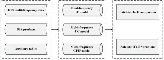
2.1. Dual-Frequency IF Model

In terms of BDS-3 data processing, the IGS ACs (Analysis Centers) commonly incorporate B1I and B3I dual-frequency signals. To be consistent with the IGS ACs’ convention, the dual-frequency IF combined clock with B1I/B3I signals, which assimilates code hardware delays on corresponding frequencies, is introduced with definition as:
c d t ^ r = c d t r + f 2 2 f 2 2 f 6 2 d r , C 2 + f 6 2 f 2 2 f 6 2 d r , C 6 c d t ^ s = c d t s + f 2 2 f 2 2 f 6 2 d C 2 s + f 6 2 f 2 2 f 6 2 d C 6 s
Inserting Equation (4) into Equation (1), the re-parameterized observation equations are obtained for B1I/B3I dual-frequency signals with IF combined model:
C 26 r s = ρ L 26 + c d t ^ r c d t ^ s + m r s z w d r + ϵ ^ r , C 26 s L 26 r s = ρ L 26 + c d t ^ r c d t ^ s + m r s z w d r + λ L C w r s λ L C N ^ r , L 26 s + ϵ r , L 26 s
where C 26 r s and L 26 r s denote the IF combinations of code and phase observations; ρ L 26 denote the IF combination of geometric distance, λ L C is the IF combined phase wavelength in meters, N ^ r , L 26 s denotes the IF combined phase ambiguity in cycles with hardware delays assimilated. Once the geometric distance is corrected with known satellite and receiver coordinates, Equation (5) becomes the traditional dual-frequency IF combined model for clock estimation. Since the 1st order ionospheric delay is eliminated, unknown parameters are largely reduced for the IF model.

2.2. Multi-Frequency UC Model

Similarly, with the IGS dual-frequency IF combined clock datum, the observation equations can be obtained for B1I/B3I/B1C/B2a quad-frequency signals:
C 2 r s = ρ L 2 + c d t ^ r c d t ^ s + f 2 2 f 2 2 I ^ r , L 2 s + m r s z w d r + ϵ ^ r , C 2 s C 6 r s = ρ L 6 + c d t ^ r c d t ^ s + f 2 2 f 6 2 I ^ r , L 2 s + m r s z w d r + ϵ ^ r , C 6 s C 1 r s = ρ L 1 + c d t ^ r c d t ^ s + I F C B r , L 1 I F C B L 1 s + f 2 2 f 1 2 I ^ r , L 2 s + m r s z w d r + ϵ ^ r , C 1 s C 5 r s = ρ L 5 + c d t ^ r c d t ^ s + I F C B r , L 5 I F C B L 5 s + f 2 2 f 5 2 I ^ r , L 2 s + m r s z w d r + ϵ ^ r , C 5 s L 2 r s = ρ L 2 + c d t ^ r c d t ^ s f 2 2 f 2 2 I ^ r , L 2 s + m r s z w d r + λ 2 w r s λ 2 N ^ r , L 2 s + ϵ r , L 2 s L 6 r s = ρ L 6 + c d t ^ r c d t ^ s f 2 2 f 6 2 I ^ r , L 2 s + m r s z w d r + λ 6 w r s λ 6 N ^ r , L 6 s + ϵ r , L 6 s L 1 r s = ρ L 1 + c d t ^ r c d t ^ s + I F C B r , L 1 I F C B L 1 s f 2 2 f 1 2 I ^ r , L 2 s + m r s z w d r + λ 1 w r s λ 1 N ^ r , L 1 s + ϵ r , L 1 s L 5 r s = ρ L 5 + c d t ^ r c d t ^ s + I F C B r , L 5 I F C B L 5 s f 2 2 f 5 2 I ^ r , L 2 s + m r s z w d r + λ 5 w r s λ 5 N ^ r , L 5 s + ϵ r , L 5 s
where   * ^ r , * s is the modified parameter with hardware delays assimilated; I F C B r , L i and I F C B L i s are the receiver and satellite IFCBs (Inter-Frequency Clock Biases). Since the IFCB can in principle be expressed as linear combinations of the hardware delays on corresponding frequencies, the resulting IFCB estimates will be close to zero once the raw observations are corrected with external observation-specific biases. With geometric distances fixed with known satellite and receiver coordinates, Equation (6) becomes the UC model for multi-frequency clock and IFCB estimation.

2.3. Multi-Frequency GFIF Model

Based on Equation (1), the GFIF combination, which is commonly used for multi-frequency signal consistency analysis, can be easily accessed for B1I/B3I/B1C and B1I/B3I/B2a triple-frequency signals:
C 261 r s = ρ L 261 + f 1 2 f 1 2 f 6 2 I F C B r , L 1 f 1 2 f 1 2 f 6 2 I F C B L 1 s + ϵ r , C 261 s L 261 r s = ρ L 261 + f 1 2 f 1 2 f 6 2 I F C B r , L 1 f 1 2 f 1 2 f 6 2 I F C B L 1 s + B L 261 + ϵ r , L 261 s C 265 r s = ρ L 265 + f 5 2 f 2 2 f 5 2 I F C B r , L 5 f 5 2 f 2 2 f 5 2 I F C B L 5 s + ϵ r , C 265 s L 265 r s = ρ L 265 + f 5 2 f 2 2 f 5 2 I F C B r , L 5 f 5 2 f 2 2 f 5 2 I F C B L 5 s + B L 265 + ϵ r , L 265 s
where C * r s and L * r s are the GFIF combinations of code and phase observations; ρ L * is the GFIF combination of geometric distance; B L * is the GFIF combination of phase ambiguity in meters; ϵ r , C * s and ϵ r , L * s denote the GFIF combinations of code and phase residuals.
The GFIF combinations of geometric distances can be further written as:
ρ L 261 = f 1 2 f 1 2 f 6 2 ρ L 1 + f 6 2 f 1 2 f 6 2 ρ L 6 f 2 2 f 2 2 f 6 2 ρ L 2 f 6 2 f 2 2 f 6 2 ρ L 6 ρ L 265 = f 2 2 f 2 2 f 5 2 ρ L 2 + f 5 2 f 2 2 f 5 2 ρ L 5 f 2 2 f 2 2 f 6 2 ρ L 2 f 6 2 f 2 2 f 6 2 ρ L 6
Combining Equations (3) and (8), the GFIF combination of geometric distances can be simplified as:
ρ L 261 = f 1 2 f 1 2 f 6 2 e r s R S C F E C F P C O L 1 s e r s R E N U E C F P C O r , L 1 + f 6 2 f 1 2 f 6 2 e r s R S C F E C F P C O L 6 s e r s R E N U E C F P C O r , L 6 f 2 2 f 2 2 f 6 2 e r s R S C F E C F P C O L 2 s e r s R E N U E C F P C O r , L 2 f 6 2 f 2 2 f 6 2 e r s R S C F E C F P C O L 6 s e r s R E N U E C F P C O r , L 6 ρ L 265 = f 2 2 f 2 2 f 5 2 e r s R S C F E C F P C O L 2 s e r s R E N U E C F P C O r , L 2 + f 5 2 f 2 2 f 5 2 e r s R S C F E C F P C O L 5 s e r s R E N U E C F P C O r , L 5 f 2 2 f 2 2 f 6 2 e r s R S C F E C F P C O L 2 s e r s R E N U E C F P C O r , L 2 f 6 2 f 2 2 f 6 2 e r s R S C F E C F P C O L 6 s e r s R E N U E C F P C O r , L 6
As indicated by Equation (9), only frequency-dependent terms, i.e. PCO corrections, are remaining in GFIF combinations. Within IGS ACs’ routine multi-GNSS data processing, antenna-related corrections are commonly extracted from the igs14.atx file. However, the receiver antenna calibrations are absent in igs14.atx for BDS-3 signals. As a result, the corresponding GPS L1/L2 values are used for adjacent BDS-3 frequencies. Unlike the situation at the receiver end, the satellite antenna information for BDS-3 B1I/B3I/B1C signals is released in the igs14.atx file. The missing values for B2a signals can be filled with the corresponding B2b values considering the frequency proximity. Obviously, the PCO errors at either satellite or receiver end will be projected into line-of-sight observations. The estimation of either satellite clock or IFCB will then be contaminated by the PCO errors.
Once the geometric distance for each frequency is known precisely, the GFIF combination of geometric distances can be safely reduced from Equation (7). Then, the GFIF combinations for B1I/B3I/B1C and B1I/B3I/B2a signals can be derived as:
C 261 r s = f 1 2 f 1 2 f 6 2 I F C B r , L 1 f 1 2 f 1 2 f 6 2 I F C B L 1 s + ϵ r , C 261 s L 261 r s = f 1 2 f 1 2 f 6 2 I F C B r , L 1 f 1 2 f 1 2 f 6 2 I F C B L 1 s + B L 261 + ϵ r , L 261 s C 265 r s = f 5 2 f 2 2 f 5 2 I F C B r , L 5 f 5 2 f 2 2 f 5 2 I F C B L 5 s + ϵ r , C 265 s L 265 r s = f 5 2 f 2 2 f 5 2 I F C B r , L 5 f 5 2 f 2 2 f 5 2 I F C B L 5 s + B L 265 + ϵ r , L 265 s
With IFCBs and ambiguity terms remaining, Equation (10) becomes the GFIF model for IFCB estimation. While the IFCB can be generated from either the UC model as Equation (6) or the GFIF model as Equation (10), the results will be identical only if the applied corrections, mainly PCO corrections, are consistent. With the GFIF combination commonly formed without correcting PCOs, the resulting IFCB will derivate from that with the UC model. The disagreement may further increase once incorrect PCOs are applied in the UC model.

2.4. Clock and IFCB Estimation

Finally, the overall flow chart for real-time BDS-3 clock and IFCB estimation is illustrated in Figure 1. The whole processing consists of two main procedures, i.e., data preprocessing and parameter estimation. The raw observations are firstly corrected for biases and errors. In the data preprocessing, the phase cycle slips are detected with the MW (Melbourne-Wübbena) and GF (Geometry-Free) combination. Then, with cleaned raw observations, the parameter estimation with various models developed above, including the IF model, the UC model and the GFIF model, are conducted to obtain the real-time clock and IFCB solutions. To reduce the side effect of remaining bad observations after data preprocessing, the post-fit residuals are edited with predefined empirical thresholds. The corresponding observation noises for linear combinations can be mapped from that of raw observations following the law of error propagation. Obviously, linear correlations exist between the satellite and receiver clock/IFCB parameters. To remove the intrinsic rank deficiencies, clock and IFCB datums, such as the constellation zero-mean constraint, should be introduced.

3. Results and Discussion

To validate the developed models for real-time BDS-3 clock and IFCB estimation, RINEX3 (Receiver INdependent EXchange format 3) observation data from about 80 globally distributed IGS network stations (Figure 2) spanning 1 April to 8 April 2021 are used for the simulated real-time numerical experiments. All of the stations are able to track BDS-3 quad-frequency signals. As mentioned in the previous section, the satellite antenna information for BDS-3 B1I/B3I/B1C signals is available in the igs14.atx file, the corresponding values for the receiver antenna are still missing. However, within the igsR3.atx file for the IGS 3rd reprocessing campaign (http://acc.igs.org/repro3/repro3.html accessed on 29 January 2021), the antenna calibrations of about 40 stations, which are equipped with SEPT POLARX5 or SEPT POLARX5TR receivers, are made available for BDS-3 B1I/B3I/B1C/B2a signals. Taking account of the limited receivers with BDS-3 quad-frequency antenna information, the igs14.atx file is used when conducting clock estimation with the UC model, and the igsR3.atx file is used for IFCB determination with the GFIF model due to the smaller number of unknowns. Furthermore, to be consistent with the IGS ACs’ clock definition, the code observations are corrected with the code bias product in OSB (Observation Specific Bias) format from CAS (Chinese Academy of Sciences). The detailed processing strategy and filter settings are summarized in Table 1 and Table 2, respectively. The post-processed solutions from IGS ACs are used for clock accuracy assessment with the commonly used DD (Double-Difference) method to remove the clock datum differences. Given the DBD (Day Boundary Discontinuities) of post-processed clocks, the clock STD will be calculated on a daily basis. In all, 24 BDS-3 MEO satellites, well-distributed on three orbital planes, will be the focus of this study. The UC models with B1I/B3I dual-frequency signals, B1C/B2a dual-frequency signals, B1I/B3I/B1C triple-frequency signals, B1I/B3I/B2a triple-frequency signals and B1I/B3I/B1C/B2a quad-frequency signals are conducted for real-time BDS-3 clock and IFCB estimation. For comparison, the IF model with B1I/B3I dual-frequency signals is performed in addition to the five UC models.

3.1. Satellite Clock Comparison

The real-time DD clock time series with dual-frequency and multi-frequency signals are depicted in Figure 3 and Figure 4, respectively. Apart from the convergence part on the first day, the DD clocks show an apparent DBD phenomenon. Two potential reasons may contribute to the clock DBD. First, the reference clocks, which are generated on a daily basis, will experience jumps at day boundaries and then impact the resulting DD clocks. Second, the real-time clocks are estimated with orbit fixed to GFZ post-processed product. The GFZ daily orbit is determined with independent 24-h observation data, and therefore will inevitably be affected by the DBD phenomena. The orbit DBD will affect the orbit interpolation around day boundaries and then have an impact on the corresponding real-time clocks.
The real-time clock solutions are similar for all of the six models with the exception of the B1C/B2a UC model. As for the other five models, while the DD clocks for most satellites fall in +/− 2.0 ns after convergence, satellite C45 shows a derivation of around 3.0 ns, which may have resulted from differences between bias products used in real-time and reference clock generation. With the convergence part neglected, the DD clocks exhibit rather high intra-day stability, which indicates a small STD value compared to the corresponding RMS value. Unlike diversities among satellites with the other five models, the DD clocks with the B1C/B2a UC model fall into two distinct groups, which vary between +1.2 ns and −0.8 ns. When further examining the satellite types it is found that the two groups correspond to satellites manufactured by the CAST (China Academy of Space Technology) and the SECM (Shanghai Engineering Center for Microsatellites), respectively. Since the GFZ post-processed clock is based on B1I/B3I signals, the intra-day stability of DD clocks with the B1C/B2a UC model suggests good consistency between the B1I/B3I and B1C/B2a signals. Moreover, we must emphasize that the satellite PCO corrections for the B2a signal are absent in the igs14.atx file and replaced with corresponding B2b values in the study. Being aware of this kind of model imperfection, the consistency between the B1I/B3I UC model and the B1C/B2a UC model is really inspiring.
The daily STD values averaged over the last 6 days are depicted in Figure 5 for all of the six models. The STD values are generally less than 0.05 ns, except for satellite C45 with the B1I/B3I/B1C and B1I/B3I/B1C/B2a UC models. The variation of STD values between each model is less than 0.01 ns with the exception of satellite C45. The largest STD value difference between the six models appears for satellite C45, for which the STD value with the B1C/B2a UC model is about 0.015 ns smaller than that with the B1I/B3I/B2a model. In all, the high accuracy and consistency of the real-time clock are clearly visible for all six models, which confirms the feasibility of the developed multi-frequency UC models. The constellation-mean STD values over the experimental period are summarized in Table 3. The statistics generally coincide with those inferred from Figure 5. The relatively larger STD values for the first day are the result of the real-time filter convergence as shown in Figure 3 and Figure 4.

3.2. Satellite IFCB Characteristic

As by-products of clock estimation with multi-frequency signals, the satellite and receiver IFCBs are principally linear combinations of corresponding hardware delays. With the code hardware delays corrected at the satellite end, the resulting satellite IFCBs between the third signal B1C or B2a and the datum signals B1I and B3I are thought to be with a small deviation from zero. The satellite IFCBs between the B1C/B2a and B1I/B3I signals are presented in Figure 6 and Figure 7 for the UC models with multi-frequency signals. The satellite IFCBs are generally less than 0.2 m, which confirms the inference above. While not explicitly shown here, the satellite IFCB differences are well below 1.0 cm between both models. Leaving out the convergence part, no obvious periodical signals are observed for the resulting satellite IFCBs between the B1C and B1I/B3I signals. However, apparent nearly diurnal variations with peak-valley values reaching 3.0 cm are found for the satellite IFCBs between the B2a and B1I/B3I signals. Recalling Equation (6) for multi-frequency data processing, we speculate that one of the main contributions is the inaccuracy of satellite and receiver PCO corrections applied for the B2a signal.
To further analyze satellite IFCB between the B2a and B1I/B3I signals, the IFCB estimation is conducted with the GFIF combination. Considering the handling of satellite and receiver PCO corrections, three different strategies, including both satellite and receiver PCO-corrected (as a benchmark), only receiver PCO-corrected and both satellite and receiver PCO-uncorrected, are adopted to obtain the satellite IFCB. As shown in Figure 8, the generated satellite IFCB with satellite and receiver PCO-corrected are very similar to those in Figure 7. This kind of similarity can be fully explained with the underlying equivalence of the UC and GFIF models. When it comes to the satellite IFCB with only receiver PCO-corrected in Figure 9, no clear differences can be observed compared to the benchmark ones. However, as shown in Figure 10, further ignoring the receiver PCO in the GFIF model leads to obviously more stable satellite IFCB estimations, which suggests the aforementioned temporal variations are mainly originated from incorrect PCO corrections at the receiver end. Moreover, the reduction of nearly diurnal signals in satellite IFCB with PCOs uncorrected suggests that the GFIF combinations of satellite and receiver PCO corrections should be close to, if not exactly equal to zero in Equation (9). In general, the temporal stability of satellite IFCB based on the GFIF model confirms the consistency between the B2a and B1I/B3I signals.
While the satellite IFCB shown in Figure 10 is already much more stable than the original ones in Figure 8, the underlying basis is that the GFIF combinations of PCO corrections can be fully ignored. However, the assumption is hardly valid in theory and the residual small variations for some satellites in Figure 10 confirm its failure. To further investigate the residual signals in the satellite IFCB, we here further use the PCO information in the igsR3.atx file to conduct IFCB estimations with the GFIF model. The resulting satellite IFCB is shown in Figure 11. Because of the relatively smaller number of stations used (about half of that for Figure 8, Figure 9 and Figure 10), there exists a re-convergence on 6 April for one single satellite and the other satellites experience tiny jumps due to the zero-mean constellation constraint. Except for the re-convergence, the temporal variations are generally disappeared for all satellites compared to Figure 10, which clearly demonstrates the consistency between the B2a and B1I/B3I signals. From the above analysis, we can conclude that the deficiency of antenna information will destroy model completeness and then impede GNSS applications with multi-frequency signals.

4. Conclusions

In this study, we thoroughly discussed the real-time BDS-3 clock estimation with multi-frequency uncombined signals. The multi-frequency UC model is first developed with B1I/B3I IF combined clock datum and then the GFIF model is derived for IFCB estimations. With data from about 80 global IGS network stations over one week, the simulated real-time numerical experiments are conducted for validation and analysis. The results indicate that the satellite clock estimation from multi-frequency UC models achieves high agreement with that from the traditional dual-frequency IF combined model. The STD of DD clocks reaches about 0.03 ns with respect to post-processed solutions. Different from the steady satellite IFCBs between the B1C and B1I/B3I signals, the satellite IFCBs between the B2a and B1I/B3I signals showed apparent periodical variations with multi-frequency UC models. Further investigation with the GFIF model using different PCO correction strategies imply the variations mainly result from imperfect receiver PCO corrections. Therefore, we address the urgency for receiver antenna information to achieve utmost accuracy in the multi-frequency data processing.

Author Contributions

Conceptualization, K.K. and J.W.; methodology, K.K.; software, K.K.; validation, K.K.; formal analysis, K.K.; investigation, K.K.; resources, K.K.; data curation, K.K.; writing—original draft preparation, K.K.; writing—review and editing, K.K., J.W. and H.H.; visualization, K.K.; supervision, J.W.; project administration, J.W. and K.K.; funding acquisition, J.W., H.H. and K.K. All authors have read and agreed to the published version of the manuscript.

Funding

This research was funded by the National Natural Science Foundation of China (Grant No. 41874029, Grant No. 41904029) and the Young Teachers Research Capability Enhancement Program of Beijing University of Civil Engineering and Architecture (Grant No. X21020).

Data Availability Statement

The observation data and precise products used in the research are available on the FTP of Wuhan University (ftp://igs.gnsswhu.cn/pub/ accessed on 29 January 2021).

Acknowledgments

The authors gratefully acknowledge IGS for providing the observation data and GFZ for providing the precise products.

Conflicts of Interest

The authors declare no conflict of interest.

References

  1. Johnston, G.; Riddell, A.; Hausler, G. The International GNSS Service. In Springer Handbook of Global Navigation Satellite Systems; Springer Science and Business Media LLC: Berlin/Heidelberg, Germany, 2017; pp. 967–982. [Google Scholar]
  2. Deng, Z.; Fritsche, M.; Nischan, T.; Bradke, M. Multi-GNSS Ultra Rapid Orbit-, Clock- & EOP-Product Series. GFZ Data Serv. 2016. [Google Scholar] [CrossRef]
  3. Bock, H.; Dach, R.; Jäggi, A.; Beutler, G. High-rate GPS clock corrections from CODE: Support of 1 Hz applications. J. Geod. 2009, 83, 1083–1094. [Google Scholar] [CrossRef] [Green Version]
  4. Hauschild, A.; Montenbruck, O. Kalman-filter-based GPS clock estimation for near real-time positioning. GPS Solut. 2008, 13, 173–182. [Google Scholar] [CrossRef]
  5. Gong, X.; Gu, S.; Lou, Y.; Zheng, F.; Ge, M.; Liu, J. An efficient solution of real-time data processing for multi-GNSS network. J. Geod. 2017, 92, 797–809. [Google Scholar] [CrossRef]
  6. Li, X.; Xiong, Y.; Yuan, Y.; Wu, J.; Li, X.; Zhang, K.; Huang, J. Real-time estimation of multi-GNSS integer recovery clock with undifferenced ambiguity resolution. J. Geod. 2019, 93, 2515–2528. [Google Scholar] [CrossRef]
  7. Fu, W.; Huang, G.; Zhang, Q.; Gu, S.; Ge, M.; Schuh, H. Multi-GNSS real-time clock estimation using sequential least square adjustment with online quality control. J. Geod. 2018, 93, 963–976. [Google Scholar] [CrossRef]
  8. Zhao, Q.; Sun, B.; Dai, Z.; Hu, Z.; Shi, C.; Liu, J. Real-time detection and repair of cycle slips in triple-frequency GNSS measurements. GPS Solut. 2014, 19, 381–391. [Google Scholar] [CrossRef]
  9. Li, T.; Melachroinos, S. An enhanced cycle slip repair algorithm for real-time multi-GNSS, multi-frequency data processing. GPS Solut. 2019, 23, 1. [Google Scholar] [CrossRef]
  10. Geng, J.; Bock, Y. Triple-frequency GPS precise point positioning with rapid ambiguity resolution. J. Geod. 2013, 87, 449–460. [Google Scholar] [CrossRef]
  11. Li, X.; Li, X.; Liu, G.; Yuan, Y.; Freeshah, M.; Zhang, K.; Zhou, F. BDS multi-frequency PPP ambiguity resolution with new B2a/B2b/B2a + b signals and legacy B1I/B3I signals. J. Geod. 2020, 94, 107. [Google Scholar] [CrossRef]
  12. Schönemann, E.; Becker, M.; Springer, T. A new Approach for GNSS Analysis in a Multi-GNSS and Multi-Signal Environment. J. Géod. Sci. 2011, 1, 204–214. [Google Scholar] [CrossRef] [Green Version]
  13. Strasser, S.; Mayer-Gürr, T.; Zehentner, N. Processing of GNSS constellations and ground station networks using the raw observation approach. J. Geod. 2018, 93, 1045–1057. [Google Scholar] [CrossRef] [Green Version]
  14. Lu, M.; Li, W.; Yao, Z.; Cui, X. Overview of BDS III new signals. Navigation 2019, 66, 19–35. [Google Scholar] [CrossRef] [Green Version]
  15. Jin, S.; Su, K. PPP models and performances from single- to quad-frequency BDS observations. Satell. Navig. 2020, 1, 16. [Google Scholar] [CrossRef]
  16. Li, R.; Wang, N.; Li, Z.; Zhang, Y.; Wang, Z.; Ma, H. Precise orbit determination of BDS-3 satellites using B1C and B2a dual-frequency measurements. GPS Solut. 2021, 25, 95. [Google Scholar] [CrossRef]
  17. Fu, W.; Wang, L.; Chen, R.; Han, Y.; Zhou, H.; Li, T. Combined BDS-2/BDS-3 real-time satellite clock estimation with the overlapping B1I/B3I signals. Adv. Space Res. 2021, 68, 4470–4483. [Google Scholar] [CrossRef]
  18. Montenbruck, O.; Hauschild, A.; Steigenberger, P.; Langley, R.B. Three’s the challenge: A close look at GPS SVN62 triple-frequency signal combinations finds carrier-phase variations on the new L5. GPS World 2010, 21, 8–19. [Google Scholar]
  19. Li, X.; Hu, X.; Guo, R.; Tang, C.; Zhou, S.; Liu, S.; Chen, J. Orbit and Positioning Accuracy for New Generation Beidou Satellites during the Earth Eclipsing Period. J. Navig. 2018, 71, 1069–1087. [Google Scholar] [CrossRef]
  20. Saastamoinen, J. Atmospheric correction for the troposphere and stratosphere in radio ranging satellites. Bull. Géodésique 1972, 15, 247–251. [Google Scholar] [CrossRef]
  21. Davis, J.L.; Herring, T.A.; Shapiro, I.I.; Rogers, A.E.E.; Elgered, G. Geodesy by radio interferometry: Effects of atmospheric modeling errors on estimates of baseline length. Radio Sci. 1985, 20, 1593–1607. [Google Scholar] [CrossRef]
  22. Böhm, J.; Moeller, G.; Schindelegger, M.; Pain, G.; Weber, R. Development of an improved empirical model for slant delays in the troposphere (GPT2w). GPS Solut. 2015, 19, 433–441. [Google Scholar] [CrossRef] [Green Version]
  23. Böhm, J.; Werl, B.; Schuh, H. Troposphere mapping functions for GPS and very long baseline interferometry from European Centre for Medium-Range Weather Forecasts operational analysis data. J. Geophys. Res. Solid Earth 2006, 111, B02406. [Google Scholar] [CrossRef]
  24. Petit, G.; Luzum, B. (Eds.) IERS Conventions; Verlag des Bundesamts für Kartographie und Geodäsie: Frankfurt, Germany, 2010. [Google Scholar]
  25. Lyard, F.; Lefevre, F.; Letellier, T.; Francis, O. Modelling the global ocean tides: Modern insights from FES2004. Ocean Dyn. 2006, 56, 394–415. [Google Scholar] [CrossRef]
  26. Wu, J.T.; Wu, S.C.; Hajj, G.A.; Bertiger, W.I.; Lichten, S.M. Effects of antenna orientation on GPS carrier phase. Manuscr. Geod. 1993, 18, 91–98. [Google Scholar]
Figure 1. Flow chart for real-time BDS-3 clock and IFCB estimation.
Remotesensing 14 00966 g001
Figure 2. Stations for real-time BDS-3 clock and IFCB estimation, the blue and red icons denote receivers without and with antenna calibrations for BDS-3 multi-frequency signals, respectively.
Remotesensing 14 00966 g002
Figure 3. Real-time satellite clock with dual-frequency signals, the top one denotes IF model with B1I/B3I signals, the middle one denotes UC model with B1I/B3I signals, the bottom one denotes UC model with B1C/B2a signals.
Remotesensing 14 00966 g003
Figure 4. Real-time satellite clock with multi-frequency signals, the top one denotes UC model with B1I/B3I/B1C signals, the middle one denotes UC model with B1I/B3I/B2a signals, the bottom one denotes UC model with B1I/B3I/B1C/B2a signals.
Remotesensing 14 00966 g004
Figure 5. STD of real-time satellite clock with different model, the top one denotes satellite clock STD with dual-frequency signals, the bottom one denotes satellite clock STD with multi-frequency signals.
Remotesensing 14 00966 g005
Figure 6. Real-time satellite IFCB for B1C and B1I/B3I signals, the top one denotes results with B1I/B3I/B1C triple-frequency UC model, the bottom one denotes results with B1I/B3I/B1C/B2a quad-frequency UC model.
Remotesensing 14 00966 g006
Figure 7. Real-time satellite IFCB for B2a and B1I/B3I signals, the top one denotes results with B1I/B3I/B2a triple-frequency UC model, the bottom one denotes results with B1I/B3I/B1C/B2a quad-frequency UC model.
Remotesensing 14 00966 g007
Figure 8. Real-time satellite IFCB for B2a and B1I/B3I signals with GFIF model, the satellite and receiver PCOs are corrected with igs14.atx, the values for each satellite are shifted by multiple of 0.05 m for clarity.
Remotesensing 14 00966 g008
Figure 9. Real-time satellite IFCB for B2a and B1I/B3I signals with GFIF model, the satellite PCO is corrected with igs14.atx, the receiver PCO is uncorrected, the values for each satellite are shifted by multiplier of 0.05 m for clarity.
Remotesensing 14 00966 g009
Figure 10. Real-time satellite IFCB for B2a and B1I/B3I signals with GFIF model, the satellite and receiver PCOs are uncorrected, the values for each satellite are shifted by multiplier of 0.05 m for clarity.
Remotesensing 14 00966 g010
Figure 11. Real-time satellite IFCB for B2a and B1I/B3I signals with GFIF combination, the satellite and receiver PCOs are corrected with igsR3.atx, the values for each satellite are shifted by multiplier of 0.05 m for clarity.
Remotesensing 14 00966 g011
Table 1. Processing strategy for real-time BDS-3 clock and IFCB estimation.
ItemsModels
Basic observablesRaw code and phase; cut-off elevation: 10.0 deg; sampling rate: 30.0 s
Weighting strategyCode: 0.3 m; phase: 0.3 cm; the sigma increases with decreasing elevation angle using the function 1/sin(elevation)
Antenna phase centerIF/UC model for clock estimation: corrected with PCO and PCV values from igs14.atx file, GPS values adopted for BDS-3 at the receiver end;
GFIF model for IFCB estimation: corrected with PCO and PCV values from either igs14.atx or igsR3.atx file
Attitude modelModeled [19]
Tropospheric delayHydrostatic part according to the formula of [20] as given by [21] with surface pressure computed with GPT2w model [22]; Wet part estimated as random walk process with VMF1 (Vienna Mapping Function 1) [23]; Horizontal gradient model not considered
Ionospheric delay1st order eliminated for IF/GFIF model and estimated for UC model, higher-order not considered
Tidal displacementsSolid Earth tides, ocean loading and pole tides according to IERS Conventions 2010 [24] with FES2004 ocean tide model [25]
Phase wind-up effectCorrected [26]
Receiver clockEstimated as white noise process
Satellite clockEstimated as white noise process
Phase ambiguitiesEstimated as constant each observation pass
Satellite orbitFixed to the post-processed solution from IGS ACs
Earth orientation parametersFixed to IERS (International Earth Rotation Service) Bulletin A
EstimatorExtended Kalman filter
Table 2. Filter setting for real-time BDS-3 clock and IFCB estimation.
ParametersInitial StateInitial VarianceProcess Noise
Satellite clockPost-processed solution1 × 104 m2-
Receiver clockSPP1 × 104 m2-
Station zenith wet delay0.0 m0.25 m23 × 10−8 × 30 m2
AmbiguityAligned to code1 × 106 m20.0 m2
Satellite IFCB0.0 m1 × 104 m2-
Receiver IFCB0.0 m1 × 104 m2-
Table 3. Constellation-mean STD of real-time satellite clock (unit: ns), the character A/B/C/D/E/F are used to denote B1/B3I IF model, B1I/B3I UC model, B1C/B2a UC model, B1I/B3I/B1C UC model, B1I/B3I/B2a UC model, B1I/B3I/B1C/B2a UC model for clarity.
Day\ModelABCDEF
April-010.0870.0870.0820.0840.0850.085
April-020.0270.0270.0330.0270.0280.028
April-030.0250.0250.0280.0250.0270.026
April-040.0300.0300.0330.0300.0300.031
April-050.0250.0250.0270.0250.0280.027
April-060.0260.0260.0280.0260.0290.028
April-070.0290.0290.0280.0290.0310.032
Publisher’s Note: MDPI stays neutral with regard to jurisdictional claims in published maps and institutional affiliations.

