An Improved Sea Ice Classification Algorithm with Gaofen-3 Dual-Polarization SAR Data Based on Deep Convolutional Neural Networks

Abstract

The distribution of sea ice is one of the major safety hazards for sea navigation. As human activities in polar regions become more frequent, monitoring and forecasting of sea ice are of great significance. In this paper, we use SAR data from the C-band synthetic aperture radar (SAR) Gaofen-3 satellite in the dual-polarization (VV, VH) fine strip II (FSII) mode of operation to study the Arctic sea ice classification in winter. SAR data we use were taken in the western Arctic Ocean from January to February 2020. We classify the sea ice into four categories, namely new ice (NI), thin first-year ice (tI), thick first-year ice (TI), and old ice (OI), by referring to the ice maps provided by the Canadian Ice Service (CIS). Then, we use the deep learning model MobileNetV3 as the backbone network, input samples of different sizes, and combine the backbone network with multiscale feature fusion methods to build a deep learning model called Multiscale MobileNet (MSMN). Dual-polarization SAR data are used to synthesize pseudocolor images and produce samples of sizes 16 × 16 × 3, 32 × 32 × 3, and 64 × 64 × 3 as input. Ultimately, MSMN can reach over 95% classification accuracy on testing SAR sea ice images. The classification results using only VV polarization or VH polarization data are tested, and it is found that using dual-polarization data could improve the classification accuracy by 10.05% and 9.35%, respectively. When other classification models are trained using the training data from this paper for comparison, the accuracy of MSMN is 4.86% and 1.84% higher on average than that of the model built using convolutional neural networks (CNNs) and ResNet18 model, respectively.

1. Introduction

China’s polar scientific research career started in 1984, spanning roughly forty years of history so far. During this period, polar research stations such as Great Wall Station, Zhongshan Station, and Kunlun Station in Antarctica and Yellow River Station in the Arctic were established one after another, which greatly promoted the development of polar research in China. With the commissioning of the Xuelong polar research vessel, the frequency of China’s polar scientific research has also increased. As the third-generation polar icebreaker and research vessel of China, Xuelong has carried out dozens of polar research missions and covered all five oceans. However, in the process of polar research, the distribution of sea ice is often a prominent factor for the captain of a research vessel in deciding the navigation trajectory and is also one of the major safety hazards of ship navigation. For example, during the 35th Antarctic scientific research mission in 2019, the Xuelong was affected by dense fog and collided with icebergs, damaging some equipment, but fortunately, no person was injured. Therefore, for safe navigation and maritime activities, high-precision sea ice monitoring and prediction of polar sea ice concentration, type, thickness, and other information are necessary. Hence, an enormous amount of research effort goes into sea ice research [1,2,3,4]. Many countries have gradually started to provide specialized sea-ice-related services. Examples include the National Ice Center (NIC) in the United States, the Canadian Ice Service (CIS) in Canada, the Arctic and Antarctic Research Institute (AARI) in Russia, and the Norwegian Ice Service (NIS) in Norway. Besides, ice maps containing information on sea ice concentration and type are regularly published for marine navigation and other activities according to the standards set by the World Meteorological Organization [5].

Synthetic aperture radar can provide all-day, all-weather high-resolution radar images, which is an excellent way to observe sea ice. Numerous articles use SAR data as the data source of sea ice observation [6,7]. According to the principle of synthetic aperture radar imaging, the backscattering coefficients of sea ice in different stages of development are different. For example, primary ice with a smooth surface usually has a small backscattering coefficient and often appears as a darker area in the image, while multiyear ice with a rough surface is brighter in the image. The difference in gray values in the images is an important indicator used to distinguish sea ice types. Furthermore, the development of polarization SAR provides a new and more effective solution for sea ice classification. Gill et al. found that the accuracy of the maximum likelihood classifier improved when uncorrelated polarization parameters were used [8]. A. Malin Johansson et al. used SAR data of multiple polarizations and multiple bands to study the relationship between scattering entropy and copolarization rate and concluded that dual-polarization (HH and VV) X-band scene data could be used to complement the full polarization C- and L-band data by restricting the full polarization dataset to the copolarization channel to improve the signal-to-noise ratio and thus the accuracy [9]. Liu Huiying et al. calculated the gray-scale cogeneration matrix of SAR images by using dual-polarization Radarsat-2 ScanSAR data to extract the texture features of sea ice, and finally, the SVM classifier effect was further optimized [10].

In traditional sea ice classification, the commonly used features include backscattering coefficient [11], texture features [10,12,13,14], polarization parameter features [15,16], and time–space features [17]. Algorithms such as decision trees and random forests [18,19], support vector machines [10,20], neural networks, and bayesian classifiers [21] are widely used classifiers. However, with the rise of deep learning methods, convolutional neural networks can often achieve better results in image classification tasks. In recent years, sea ice classification methods based on deep learning have emerged in an endless stream. Hugo Boulze et al. built out two datasets from the 2018 and 2020 Sentinel-1 scanning mode images, using CIS ice maps as real data and a simple network built with CNN as a classifier, for which the accuracies of old ice (OI) and first-year ice (FY) are 98% and 85%, respectively [22]. Song Wei et al. used the ResNet method and achieved over 90% accuracy in FYI, but the accuracy in young ice (YI) was generally less than 80% [23]. Yanling Han et al. achieved more than 95% FYI classification accuracy using heterogeneous data fusion and deep learning method, but optical images of the same time and place were indispensable [24]. Tianyu Zhang et al. simplified the ResNet network structure and used the full polarization strip mode data of the Gaofen-3 satellite for classification and obtained 94% accuracy. On this basis, it was verified that the network was still applicable to Sentinel-1 data [25].

The Gaofen-3 satellite is China’s first C-band multipolarization synthetic aperture radar satellite; it has 12 imaging modes, making it the SAR satellite with the most imaging modes in the world. With a resolution of 1–500 m and a width of 10–650 km, the satellite can meet the needs of various scenarios. As the first civil SAR satellite in China, Gaofen-3 has been widely used in various fields, including disaster prevention and mitigation, ocean observation, and environmental monitoring, improving the investigation and monitoring capabilities of various industries [26]. The Gaofen-3 satellite has provided a large amount of data support for scientific research activities in various fields, such as ship detection [27,28], feature classification [29], and water body extraction [30]. Our research is funded by the National Key Research and Development Program, and we can use the data reception and processing system of the Gaofen-3 satellite to process raw data. Besides, fine strip II (FSII) data have a resolution better than 10 m, a swath of about 100 km, and an incidence range of 19–50°; FSII data are often applied to the observation of ice ribs, sea ice, coast, and water bodies and are suitable for sea ice classification. Therefore, we choose Gaofen-3 satellite FSII data as our data source.

The primary objective of this paper is to explore a high-precision classification algorithm for Arctic winter sea ice using Gaofen-3 dual-polarization FSII data. First, the sea ice categories on the SAR images are broadly labeled with reference to the ice charts provided by CIS. After that, the labeled images are corrected by manual visual interpretation to generate the sample data for training. We use MobileNetV3 as the backbone network, combining multisize samples and multiscale feature fusion methods to build a deep learning network. Finally, we compare the final classification results with the algorithm in [22] and the ResNet18 classification algorithm. The algorithm in [22] is composed of several convolutional layers, so we call it small CNN (SCNN) in this paper.

2. Study Area and Data Preprocessing

2.1. Study Area and Data

We have selected 19 views of the Gaofen-3 dual-polarization FSII data, all located within the range of 145°W–85°W and 70°N–80°N, an area referred to as the Western Arctic by CIS and for which ice charts are available specifically. The spatial distribution of the 19 images is shown in Figure 1. The area covered by the orange box is used for training and the area covered by the yellow box is used for testing. All images were taken between January and February 2020; their resolution was 2.2 m in the range direction and 4.8 m in the azimuth direction. The downloaded data are all L1A-level complex images, including both the image description file and the incident angle file corresponding to each pixel. The specific image information is shown in

Table 1. Nineteen scenes of Gaofen-3 data (R for range, A for azimuth).

Id	Date	Time	Near Inc. Angle (°)	Far Inc. Angle (°)	Resolution (R × A)	Use
1	3 January 2020	02:49:28	31.34	37.97	2.25 × 4.77	train
2	4 January 2020	13:56:53	31.35	38.01	2.25 × 4.77	test
3	6 January 2020	14:14:12	31.35	38.13	2.25 × 4.78	train
4	7 January 2020	13:33:50	31.35	38.06	2.25 × 4.78	test
5	8 January 2020	02:42:28	31.34	37.92	2.25 × 4.77	train
6	8 January 2020	02:42:38	31.34	37.91	2.25 × 4.77	train
7	10 January 2020	13:08:53	31.34	38.10	2.25 × 4.78	train
8	11 January 2020	14:05:54	42.62	47.60	2.25 × 4.84	train
9	11 January 2020	14:06:09	42.62	47.60	2.25 × 4.84	train
10	11 January 2020	14:06:41	42.61	47.62	2.25 × 4.84	train
11	11 January 2020	14:07:43	42.61	47.65	2.25 × 4.84	train
12	19 January 2020	15:15:06	31.35	38.23	2.25 × 4.79	train
13	19 January 2020	15:15:57	31.36	38.23	2.25 × 4.79	train
14	19 January 2020	15:16:31	31.39	38.23	2.25 × 4.79	train
15	19 January 2020	15:16:53	31.41	38.23	2.25 × 4.79	train
16	27 January 2020	14:45:17	31.35	37.96	2.25 × 4.77	train
17	13 February 2020	16:22:47	31.34	38.08	2.25 × 4.78	train
18	21 February 2020	15:52:07	31.34	38.07	2.25 × 4.78	train
19	22 February 2020	13:30:33	31.35	38.02	2.25 × 4.78	test

. All data are downloaded from the following website: http://ids.ceode.ac.cn/ (accessed on 29 November 2021).

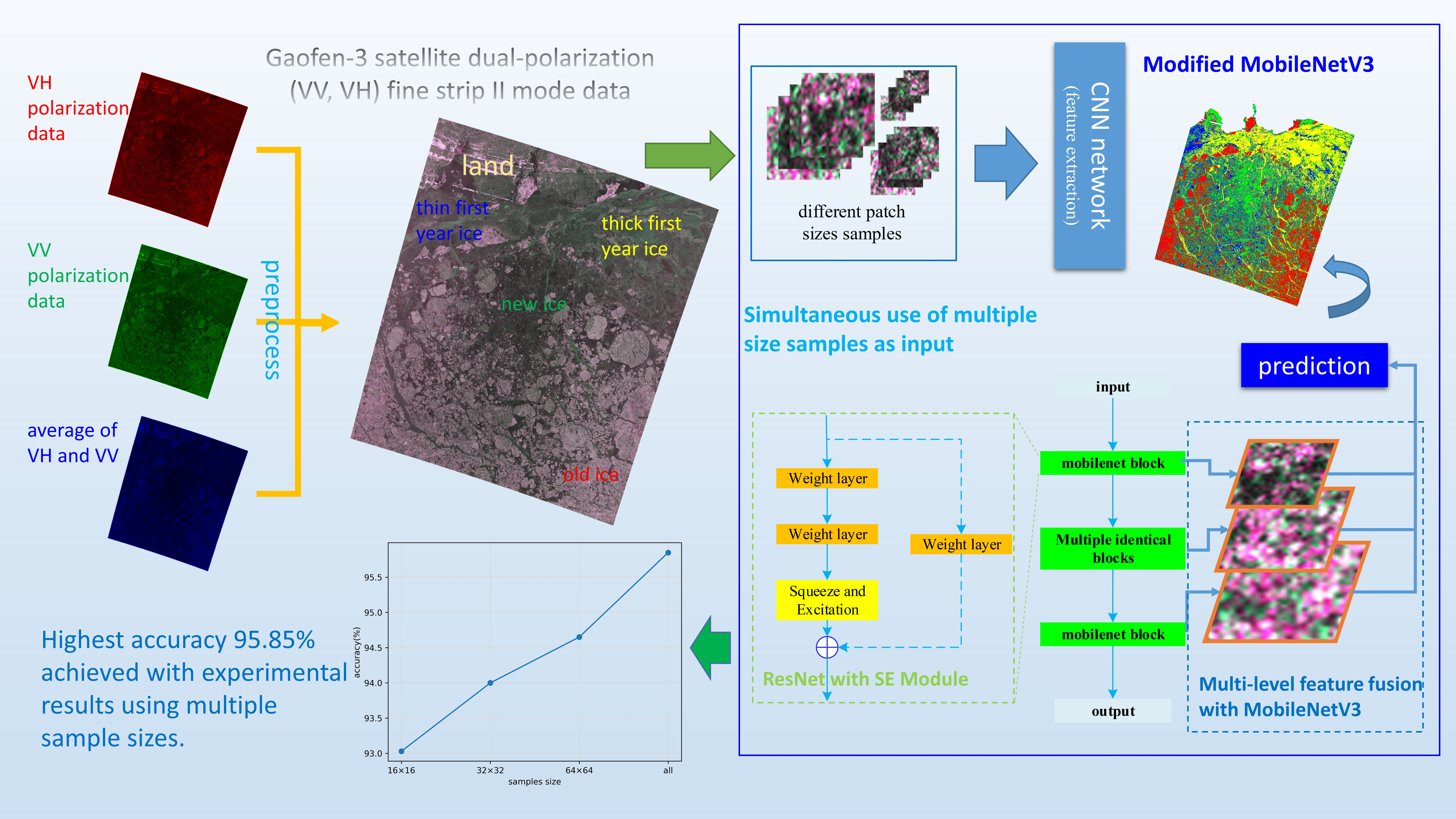
2.2. Data Preprocessing

The data preprocessing steps include radiometric calibration, speckle noise removal, gray value normalization, pseudocolor data synthesis, and training data generation. The first four steps constitute the fundamental processing requirements when using SAR data in our experiments. The formula for the Gaofen-3 radiometric calibration can be found in the Gaofen-3 user manual and is as follows:

$${\sigma }_{db}=10lo{g}_{10}(\left(P^I\right)\ast {\left(\frac{QV}{m}\right)}^2)-K_{db}$$

(1)

where ${\sigma }_{db}$ is the calibrated gray value (in decibels), $P^I$ is the gray value at each pixel of the magnitude image, m is taken as 32,767, and $K_{db}$ is the calibration constant. $QV$ (qualified value) and $K_{db}$ can be found in the description file downloaded with the Gaofen-3 data. Since there are points with zero gray value in the original image, the direct use of the original data for radiometric calibration will produce more obvious speckle noise in the output image, which will have to be removed by complex filtering later. Therefore, before radiation calibration, the pixels whose gray value is zero in the image are uniformly set to the minimum value of the pixel value other than zero in the image.

The intensity of the backscattering coefficients from water and ice surfaces is greatly affected by the incidence angle of images [31,32]. The incidence angle variation range of SAR images in scanning mode is generally a few tens of degrees, so incidence angle correction should be performed before classification [10,19,22]. In this paper, Gaofen-3 FSII data are used, whose incidence angle is roughly 31–43° and incidence angle variation range is 7–9°. To find out whether the correction of the incidence angle is needed, we calculate the relationship between the angle of incidence and the intensity of the backscattering coefficient for the selected samples. As a result, we find that there is no clear correlation between the backscattering coefficients and the incident angle of the samples. Considering that the variation of the backscattering coefficients of the selected samples at the same incident angle is relatively large, if we use a linear fitting method to correct the incident angle of the images, it will introduce a large error. Therefore, this paper does not correct the images for the incident angle.

A median filter algorithm is adopted to eliminate the effect of speckle noise, and the window size can be selected as 5 × 5. Next, dual-polarization images are synthesized into pseudocolor images using VH polarization data for the R channel, VV polarization data for the G channel, and the average of VH polarization and VV polarization data for the B channel. In the process of synthesis, the SAR image gray values are unevenly distributed, mostly concentrated in the interval of lower values, which makes the entire image darker. Therefore, in this process, the gray value of the original image is first readjusted. The adjustment strategy is to set the largest 1% of the data in the image to 65,535 and then linearly stretch the remaining 99% of the data to the interval from 0 to 65,535. The pseudocolor image is shown in Figure 2.

The ground truths are the most authoritative reference when labeling samples. However, there is almost no pixel-level sea ice product. Most of the sources of sea ice live charts come from visual interpretation [33] or expert systems [34]. Expert systems are generally used by specialized agencies and are usually not available to the public, so visual interpretation is used for the production of training data. The reference data for visual interpretation are the weekly ice charts published by CIS. The ice charts are divided into sea ice types for each region, and the ice is coded in the form of an egg code for the sea ice type. The egg code is an oval symbol based on the WMO standard, reflecting the density, stage of development (SoD), and size of the ice. For more information about the egg code, please refer to the CIS website (http://ice.glaces.ec.gc.ca/, accessed on 9 November 2021).

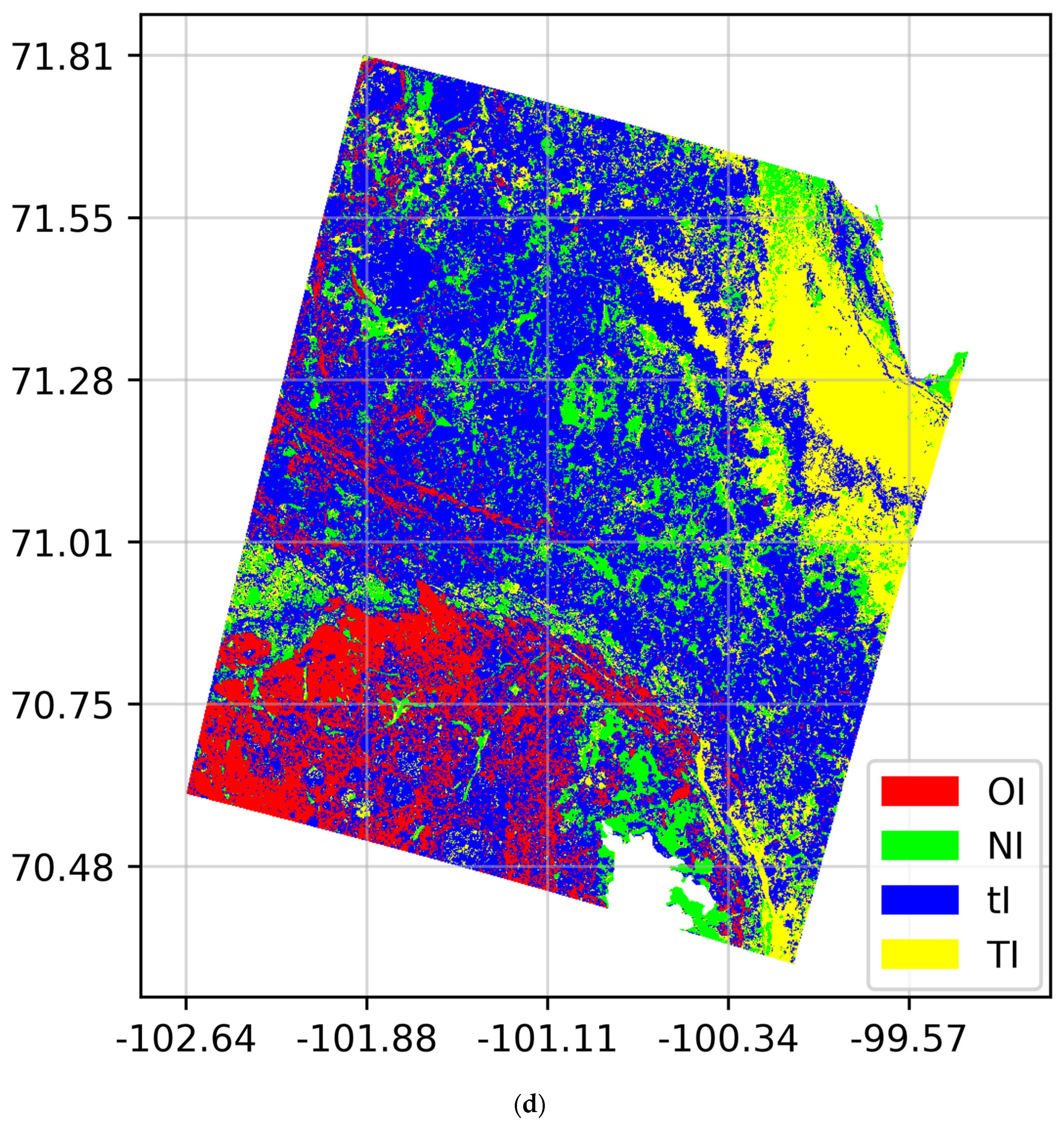
Taking scene 19 in Table 1 as an example, the process of producing the training data is as follows: According to the ice chart product released by CIS on 24 February 2020, it can be seen that the sea ice types in the region are roughly divided into three types. The sea ice type code (SoD) corresponding to the area labeled A is 7, which corresponds to the sea ice type old ice (OI). Area G has SoD codes of 7 and 4 which indicate that this area consists of two types of sea ice, with thin first-year ice (tI) numbered 7 being the dominant one. Area B with SoD code 4 corresponds to the sea ice type thick first-year ice (TI). In addition, there are a few darker areas in the images that do not belong to the above three types. In the SAR images we collected, such areas are mostly distributed along the shore or in the crevices of other types of ice. Although this type of ice is not shown on the ice map, a separate type is set up. Since the surface of primordial ice is smoother and the reflection coefficient is lower, it is tentatively considered as new ice (NI) based on its gray value. The distribution of the four types of sea ice on the SAR images is shown in Figure 3.

After determining the sea ice types and distributions, slices of each sea ice type are generated from pseudocolor images. The coordinates of each slice in the graph are recorded by randomly cropping the sliding windows of different sizes within the corresponding types of sea ice regions simultaneously. Since the randomly obtained slices may contain multiple sea ice types at the same time, it is necessary to retain the slices that can be used for the training set by manual selection. The slices are then cropped to sizes of 16 × 16 × 3, 32 × 32 × 3, and 64 × 64 × 3, respectively, to obtain the final training data, as shown in Figure 4. The red border part represents some pixels of the selected slice, the blue part is the center of the sample, and the yellow part is the current whole sample. To avoid an unbalanced sample size image training effect, the number of samples for each type of sea ice should be kept comparable as much as possible. We randomly select the data used to generate the training and test samples from the data in Table 1, and the ultimate result is scene 2, scene 4, and scene 19 for testing while the rest of the data are for training. Using the method described above, we select 35,000 training samples for each type of sea ice, of which 14% are used for validation. The training dataset is used as the input of the deep learning model so that the model gradually generates model parameters from the training data, and the validation set is used to test the accuracy of the current model continuously to avoid problems such as accuracy degradation due to overfitting.

Additional samples from scene 2, scene 4, and scene 19 are collected for testing the accuracy of the model. The number of test samples selected within each region is roughly in the range of 900–1000, with specific information shown in

Table 2. Number of samples selected for each type of sea ice test set in the three images.

Region	NI	TI	tI	OI
Scene 2	970	944	916	996
Scene 4	952	974	966	906
Scene 19	1000	1000	1000	1000

. Considering that the validation set data are continuously used to test the model accuracy during the training process, the model parameters will be adjusted accordingly to the characteristics of the validation set data, resulting in the model definitely having better results on the validation dataset. Therefore, it is more convincing to use the data not used for training to verify the accuracy of the model.

In the prediction of the whole image, the center of the sample is first determined using a sliding window of size 2 × 2 and step size 4. Then, samples of 16 × 16 × 3, 32 × 32 × 3, and 64 × 64 × 3 are cut at the same time with this window as their center. The samples with the same center are input into the model for prediction by treating the whole 64 × 64 range as the same type of sea ice. Since there are a large number of overlapping areas between different samples, the number of times each pixel is predicted as each type of sea ice is counted after the final prediction is completed for all small blocks, and the type corresponding to the maximum value is taken as the type of sea ice for that pixel.

3. Methodology

Current articles on sea ice classification algorithms based on deep learning study the effect of sample size on classification accuracy [22,25,35]. Their research approach was to select several sizes of samples to train the network to obtain the corresponding classification accuracy, using the size of the samples when the accuracy is at its highest for further study. Classification algorithms are mostly implemented as a superposition of convolutional and pooling layers [22,23,24,25,35,36]. However, we believe that it is difficult to verify the relationship between sample size and classification accuracy by only a few sets of experiments and the samples lose a large amount of spatial information after a large number of convolution and pooling operations. Therefore, we use multiple sizes of samples simultaneously to train the model while introducing a multiscale feature fusion method to take full advantage of the information contained in the feature maps and finally combine the outputs obtained by using different features to compute the final decision results.

3.1. MSMN Structure

MobileNet family of networks are lightweight networks capable of being deployed on mobile devices with fewer training parameters and low training difficulty but able to maintain a high accuracy rate. MobileNetV3 is the latest network structure of the current MobileNet family. The network introduces an attention mechanism (squeeze and excitation (SE)), which enables the network to learn the importance of each hidden layer of data automatically and assign different weights to each layer separately to improve accuracy. Since the introduction of the SE module increases the running time of the program, to achieve a balance between computational speed and classification accuracy, MobileNetV3 modifies the previous network structure to improve the running speed by reducing the number of convolutional kernels in the head from 32 to 16, removing unnecessary convolutional modules in the tail, and using a new activation function h-swish instead of the original computationally complex swish function with function 5, which eventually reduces the running speed of the program while improving the accuracy [37].

$$\mathrm{ReLU}\left(x\right)=\max \left(x,0\right)$$

(2)

$$\mathrm{ReLU}6\left(x\right)=\min \left(\mathrm{ReLU}\left(x\right),6\right)$$

(3)

$$\mathrm{swish}\left(x\right)=\frac{x}{1+e^{-x}}$$

(4)

$$\mathrm{hswish}\left(x\right)=x\frac{\mathrm{ReLU}6\left(x+3\right)}{6}$$

(5)

Figure 5 shows the structure of MSMN. The network backbone comprises roughly five parts. The input dataset containing three sizes of samples is first fed into a 3 × 3 convolutional layer to raise the number of channels to 16, which is processed by batch normalization and nonlinear activation function and used as input to the bneck module. The role of the batch normalization layer is to normalize the input data into data with Gaussian distribution between −1 and 1, avoiding the problem of gradient divergence caused by the different ranges and distributions of the data and improving the training speed. The activation function adds nonlinear features to the data to solve the problem of insufficient classification ability of the linear model. The bneck module consists of nine layers of blocks, the structure of which will be mentioned later. After the data are passed through the bneck module, the channel dimension of the data is increased to 576 using a 1 × 1 convolution operation, and then the data are fed into the batch normalization and nonlinear activation function to process the data. After that, the length and width dimensions of the data are compressed to 1 by averaging pooling, which means that the dimensions of the data become n × 1 × 1 × 576 after this operation. We added two more linear layers. The first linear layer is used to further increase the channel dimension of the data to 1280, and the second linear layer compresses the channel dimension to 4 as the backbone’s output. Other predictions come from the other output of the bneck module. The final prediction is obtained by averaging all the current predictions. Each datum in the ultimate result represents the probability that the sample belongs to the category corresponding to its subscript, and a larger value means that the sample is more likely to belong to the category corresponding to the subscript of the value. The predicted value of each sample is obtained by performing an argmax operation on the final output.

The bneck module consisting of nine block modules is the core of the network, whose overall structure is shown in Figure 5 (blue box). Different parameters input determine the function of each block module. Text displayed in the rectangular box in the figure represents from left to right the size of the convolutional kernel, the number of input channels, the number of output channels, the type of nonlinear activation function, and whether to set the SE module. In this nine-layer block, the first three layers use 3 × 3 convolutional kernels and ReLU function as the activation function, while the last six layers use 5 × 5 convolutional kernels and hswish function as the activation function. Due to the limited size of the input image, only the convolutional step size of the second and eighth layers is set to 2 to achieve downsampling. Feature maps used for feature fusion are generated from the two blocks with downsampling functionality, as shown in Figure 5 (green box). Besides, the subimage in the green dotted box comes from [38]. The small-scale feature map is first upsampled to expand itself to the same dimension as the previous level feature map. Then, the number of channels of the current feature map is made the same as the previous level feature map by 1 × 1 convolution operation. The two are superimposed to obtain the fused feature map. Each level of feature map is used separately for sea ice species prediction, and the prediction results are averaged with the results of the backbone network to obtain the final prediction results.

The block module shown in Figure 5 (red box) is a component of each layer of the bneck module, which is a two-branch structured network. The structure on the left side comprises three identical modules (the third module has no activation function), and the convolutional kernel size and activation function type are specified by the input parameters. Parameters of the SE module should be specified by the input, and “None” means that the corresponding block does not need an SE module. The design of the dotted line on the right side of the network comes from the idea of the ResNet network [39]. To avoid the features obtained by convolutional operation being too different from the input, the input data are superimposed on the output directly by the residual edge to guarantee that all features of the original data will be retained. The dotted line represents that not all blocks have this one path. Only when the convolution step is 1 and the number of input and output channels are not equal, the data need to go through the right convolution and batch normalization to complete the summation with the left data. Otherwise, without any processing, the output is directly added to the left data.

The SE module contains two main parts, squeeze and excitation, where the squeeze operation compresses the data to 1 by global average pooling for all dimensions except the channel dimension, and the fully connected layer and the activation function (excitation) are used to adjust the value of each datum. Finally, the output is obtained by multiplying the obtained data with the corresponding channels in the original data in turn. The structure of the SE module is shown in Figure 6.

Loss function plays a crucial role in the training of deep learning models. During the training process, the model is brought to the convergence state and the error of the model prediction value is reduced by minimizing the loss function. Therefore, different loss functions have a significant impact on the model. The loss function chosen in this paper is the cross-entropy loss function with the following expression:

$$\mathrm{crossentropy}=-{\displaystyle \sum }_{i=1}^{n}p\left(x_i\right)\ln \left(q\left(x_i\right)\right)$$

(6)

where $p\left(x_i\right)$ is one-hot encoded labels and $q\left(x_i\right)$ is the output of our model for each input sample. Assuming that $\mathrm{c}$ is used to represent the category of $x_i$, one-hot encode means that the label $\mathrm{c}$ is replaced with a binary vector $p\left(x_i\right)$ with length equal to the number of classes. For example, $p\left(x_i\right)=\left(1,0, 0, 0\right)$ corresponds to $\mathrm{c}=1$ (new ice). The cross-entropy loss function makes the predicted probability distribution as close as possible to the true probability distribution by reducing the difference between the two probability distributions.

The training parameters are shown in

Table 3. Configuration of parameters during model training.

Parameter	Value
Learning rate	0.01
Decay	0.00004
Batch size	64
L2 regularization coefficient γ	0.1

. The learning rate has a significant influence on the training effect of the model. A small learning rate leads to a very slow convergence process, while a large one will cause the gradient to oscillate constantly around the minimum value, which leads to no convergence. The learning rate is initially set to 0.01 and γ to 0.1 with 80 iterations, and the learning rate is adjusted at the 30th and 50th iterations, with the new learning rate being the multiplication of the previous learning rate and γ. The decay is 0.00004 and the batch size depends on the memory size, which is set to 64 in this paper. These parameters are derived from the original values during the training of the original MobileNetV3 model, and we do not consider whether these parameters are optimal for the model.

3.2. Evaluation Methodology

The confusion matrix, also known as the error matrix, is one of the standard formats for assessing accuracy. The number of rows and columns of the confusion matrix is equal to the number of categories. Each column of the confusion matrix represents the predicted category, and the total number of each column represents the number of samples predicted to be in that category; each row represents the true attribution category of the samples, and the total number of samples in each row represents the number of data instances in that category. By considering the samples belonging to this category as positive examples and those not belonging to this category as negative examples, the classification process can be considered as a dichotomy, whereupon the following evaluation metrics can be introduced: overall accuracy (Accu), single category accuracy (Prec), and Kappa coefficient.

Accu is the number of all correct classifications divided by the number of all samples. Prec is the number of correctly classified sea ice samples in a category divided by the number of samples in that category. The kappa coefficient is a measure of classification accuracy and is calculated by Equation (7):

$$\mathrm{kappa}=\frac{p_o-p_e}{1-p_e}$$

(7)

where $p_o$ is Accu and $p_e$ is calculated by Equation (8). Assuming that the number of samples of all categories is $\mathrm{n}$, the number of sample categories is $C$, $a_k$ represents the true number of samples of each category, and $b_k$ represents the number of each category in the predicted outcome where $1\le k\le C$, then

$$p_e=({\displaystyle \sum }_{k=1}^C{a}_k{b}_k)/\left(n\times n\right)$$

(8)

The evaluation process is only for the classification accuracy of sea ice, so the land part in the image is removed in advance.

4. Experimental Results and Evaluation

Three experiments are designed to evaluate the performance of MSMN. First, we compare the performance of MSMN with models trained without adding the multiscale feature fusion method using single-size samples. Second, we trained the classification model using single-polarization data alone for comparison with the model trained using dual-polarization data. Finally, to further test the classification effectiveness of the models, we trained SCNN and ResNet18 with the obtained data, plotted the confusion matrix of the classification results of these classifiers, and evaluated the performance of each classifier by comparing the three parameters mentioned in Section 3.2.

4.1. Classification Results Using Different Patch Sizes

The first three models are obtained by training with samples of the three sizes separately while the last model is MSMN. The test data are selected from scene 19 mentioned in Section 2.2. We use these data to test each of the four models, and the confusion matrix is shown in

Table 4. Confusion matrix of classification results using different patch sizes and MSMN.

Patch Size	Ice Type	NI	TI	tI	OI	Prec (%)	Accu (%)	Kappa (%)
16 × 16	NI	981	9	10	0	98.10	93.03	90.70
	TI	34	872	91	3	87.20
	tI	23	23	916	38	91.60
	OI	0	1	47	952	95.20
32 × 32	NI	977	12	11	0	97.70	94.00	92.00
	TI	20	884	93	3	88.40
	tI	14	16	921	49	92.10
	OI	0	0	22	978	97.80
64 × 64	NI	984	10	6	0	98.40	94.65	92.87
	TI	24	933	43	0	93.30
	tI	25	34	901	40	90.10
	OI	0	1	31	986	98.60
MSMN	NI	983	1	16	0	98.30	95.85	94.47
	TI	19	927	52	2	92.70
	tI	11	8	935	46	93.50
	OI	0	4	17	989	98.90

.

As is shown in Table 4, MSMN achieves the highest overall classification accuracy and kappa coefficient; the overall classification accuracy is 1.2% higher than that of the model obtained by training with 64 × 64 samples, and the kappa coefficient is 0.016 higher. This result indicates that the use of multisize samples and multiscale features can improve the classification accuracy of the model. The results from the first three models reflect that the classification accuracies of the three models increase as the sample size increases, which is attributed to the richer spatial information provided by the larger size samples. As seen in the sea ice classification of each category, the classification accuracies of NI are largely unaffected by the sample size, remaining above 97.5% in all four cases. The classification accuracies of OI increase with sample size and reach a maximum of 98.9% in the results of MSMN. The classification accuracies of TI reach the highest when using 64 × 64 samples alone, while those obtained when using 16 × 16 and 32 × 32 size samples are 6.10% and 4.90% lower, respectively, which is the reason why the classification accuracy of MSMN for TI does not reach the highest. The classification accuracies of tI reach the lowest when using samples of 64 × 64 size, indicating that large size samples are not suitable for classification of tI.

4.2. Classification Results Using Different Polarization Data

The test data are scene 19 in Table 1. The classification results of the image are shown in Figure 7 and the confusion matrix is shown in

Table 5. Confusion matrix of classification results using VH polarization, VV polarization, and dual-polarization data.

Data	Ice Type	NI	TI	tI	OI	Prec (%)	Accu (%)	Kappa (%)
VH	NI	678	320	2	0	67.80	85.80	80.84
	TI	46	924	28	2	92.40
	tI	56	24	858	70	85.80
	OI	4	0	24	972	97.20
VV	NI	992	8	0	0	99.20	86.50	82.00
	TI	32	842	64	62	84.20
	tI	48	172	680	108	68.00
	OI	2	22	30	946	94.60
VH + VV	NI	983	1	16	0	98.30	95.85	94.47
	TI	19	927	52	2	92.70
	tI	11	8	935	46	93.50
	OI	0	4	17	989	98.90

. For the next test, test samples selected from scene 19 mentioned in Section 2.2 are used to generate new samples that contain only VH polarization or VV polarization data. The new sample remains the same at 1000 of each type for testing the classification results of different polarization data.

From the confusion matrix, it can be seen that the classification accuracies are 85.80%, 86.50%, and 95.85% for the three cases, respectively. When using dual-polarization data, the overall accuracy of classification using only VH polarization data is improved by 10.05% with kappa coefficient increased by 0.1363, and the overall accuracy of classification using only VV polarization data is improved by 9.35% with kappa coefficient increased by 0.1247. It can be concluded from the above comparison that the combined use of dual-polarization data can compensate for the lack of information when single-polarization data are used alone, allowing the classifier to learn more classification basis to improve the accuracy of classification results.

The difference in overall classification accuracy between VH polarization data and VV polarization data is not significant. In terms of overall level, the numbers of features obtained by the model from these two types of data alone are roughly equivalent. Although the overall classification accuracy using single-polarization data is poor, there is still something to be said for the classification of single categories. For example, the classification accuracy of NI using only VV polarization data reached 99.2%, and the classification accuracy of OI using only VH polarization data reached 97.2%.

To further investigate the test results, we calculate the distribution of backscattering coefficients for all currently selected samples and plot box–whisker plots of backscattering coefficients for samples of four sea ice types in both polarization modes, as shown in Figure 8. The orange horizontal line in the figure represents the position of the mean value of the backscatter coefficient for this category of sea ice, the upper and lower edges of the rectangle are the upper quartile (Q3) and lower quartile (Q1) of this category of data, and the endpoints of the lines outside the rectangle represent Q3 + 1.5 × IQR and Q1 − 1.5 × IQR, where IQR = Q3 − Q1. It can be seen from the figure that the backscattering coefficients of the images in the VH polarization mode are generally lower than those of the VV polarization mode. The mean value of the backscattering coefficient for the VH polarization data is roughly distributed in the range of −30 to −20 dB with an overall value of −25 dB, while the mean value of the backscattering coefficient for the VV polarization data is distributed in the range of −25 to −10 dB with an overall value of −17 dB. The distribution patterns of the backscattering coefficients for each category are the same for both polarization modes with the mean value of OI being significantly higher than the other three categories of sea ice while the mean value of NI is slightly lower than the other three categories of sea ice. In general, the separation between the four types in the VV polarization data is slightly better than that in the VH polarization data, which results in the overall accuracy being further improved when the two polarizations are used together.

4.3. Classification Results of Different Classification Algorithms

Recently, there have been many studies using CNNs for sea ice classification, most of which achieved high accuracy [22,23,24,25,35,36]. However, the algorithms they used are not available, except for [22]. Many current deep learning network frameworks are able to achieve better results in the field of image classification, such as the experimental results of the ResNet [39] feature extraction network used by Tianyu Zhang et al. on fully polarized Gaofen-3 data. Therefore, in this paper, we use our samples to train SCNN and ResNet18 network to test the difference in performance between these two classification methods and MSMN. The SCNN network we used in [22] can be downloaded from https://github.com/nansencenter/s1_icetype_cnn/ (accessed on 21 November 2021). The training for SCNN and ResNet18 models above uses only 32 × 32 size samples.

We use the test samples mentioned in Section 2.2 selected from scene 2, scene 4, and scene 19 to test the classification effectiveness of each algorithm in three regions. Following the evaluation method mentioned in Section 3.2, the classification results are evaluated by plotting the confusion matrix of the classification results, from which three metrics of overall accuracy, single category accuracy, and kappa coefficient are calculated. The classification results of the three algorithms in three different regions are shown by three sets of figures. Figure 9, Figure 10 and Figure 11 correspond to the results of the classification algorithms in scene 2, scene 4, and scene 19, respectively. The confusion matrix of all classification results is shown in

Table 6. Sea ice classification confusion matrix using three classification algorithms in three regions.

Region	Method	Ice Type	NI	TI	tI	OI	Prec (%)	Accu (%)	Kappa (%)
Scene 2	SCNN	NI	855	101	14	0	88.14	90.17	86.90
		TI	0	810	127	7	85.81
		tI	0	51	835	30	91.16
		OI	0	0	46	950	95.38
	ResNet18	NI	963	6	1	0	99.28	94.04	92.05
		TI	39	866	36	3	91.74
		tI	22	42	803	49	87.66
		OI	0	4	26	966	96.99
	MSMN	NI	961	3	6	0	99.07	95.66	94.21
		TI	22	885	35	2	93.75
		tI	4	33	844	35	92.14
		OI	0	3	23	970	97.39
Scene 4	SCNN	NI	872	65	15	0	91.60	91.10	88.13
		TI	0	851	122	1	87.37
		tI	2	42	889	33	92.03
		OI	3	0	55	848	93.60
	ResNet18	NI	949	2	1	0	99.68	94.18	92.24
		TI	50	865	59	0	88.81
		tI	12	31	872	51	90.27
		OI	0	3	19	664	98.34
	MSMN	NI	930	7	15	0	97.69	95.37	93.82
		TI	18	902	52	2	92.61
		tI	13	22	905	26	93.69
		OI	0	4	17	885	97.68
Scene 19	SCNN	NI	944	41	15	0	94.40	91.02	88.03
		TI	0	871	125	4	87.10
		tI	2	47	898	53	89.80
		OI	3	0	69	928	92.80
	ResNet18	NI	998	2	0	0	99.80	93.13	90.83
		TI	54	868	77	1	86.80
		tI	35	25	895	45	89.50
		OI	0	0	36	964	96.40
	MSMN	NI	983	1	16	0	98.30	95.85	94.47
		TI	19	927	52	2	92.70
		tI	11	8	935	46	93.50
		OI	0	4	17	989	98.90

.

From the confusion matrix, it can be seen that MSMN can achieve the highest classification accuracy in all three regions. In scene 19, our method achieves the highest accuracy of 95.85%, which is 4.83% and 2.72% higher than SCNN and ResNet18, respectively and the kappa coefficient is 0.9447, which is 0.0644 and 0.0364 higher, respectively. In the other two sets of experiments, the numerical difference of classification accuracies between our method and the other two is slightly reduced. MSMN achieves 95.66% accuracy in scene 2, which is 5.49% and 1.62% higher than SCNN and ResNet18, respectively, with a kappa coefficient 0.0731 and 0.0216 higher, respectively. In scene 4, our method achieves 95.37% accuracy, which is 4.27% and 1.19% higher than SCNN and ResNet18, respectively, with a kappa coefficient 0.0569 and 0.0158 higher, respectively.

From the classification results of each category, SCNN can consistently maintain the classification accuracy above 90% for OI, but the classification accuracies for the other three categories are poor and irregular. ResNet18 and MSMN are comparable in classification accuracies on NI and OI, mostly reaching 97–99%. However, the classification results of ResNet18 on TI and tI are generally worse than those of MSMN. As can be seen in Table 6, the classification accuracies of ResNet18 for TI and tI are generally below 90%, while the classification accuracies of MSMN are able to stabilize at 92–93%. It is a large number of misclassifications in ResNet18 in TI and tI classification that pulls down its overall classification accuracy.

We try to analyze the above experimental results in terms of network structure. SCNN is composed of only three convolutional layers, three fully connected layers, and several pooling layers, which is a simple structure with few layers. Therefore, it is difficult to ensure that enough sample features are obtained, leading to the results being poor. The ResNet18 network obviously has a deeper level structure, and the addition of residual edges ensures the reliability of the convolutional layer obtaining sample features, so the classification accuracy is significantly improved. MSMN introduces a multiscale feature fusion method while ensuring the network depth and residual edges, which makes up for the shortcomings of ResNet18 in using only single-scale feature maps for prediction and fully exploits the utilization value of each scale of feature maps. In addition, the use of an attention mechanism enables the model to acquire information from feature maps selectively, thus improving the classification accuracy. Despite all this, the models we used have some common defects. For instance, both TI and tI are first-year ice with more complex location distribution on the image and have many similar features, making it difficult for the model to distinguish them accurately even though a multiscale feature fusion method is introduced.

5. Discussion

In this paper, we choose the Gaofen-3 dual-polarization FSII SAR data to study the classification of winter sea ice in the western Arctic Ocean. We first assume that each image contains only four types of sea ice, namely new ice, thin first-year ice, thick first-year ice, and old ice; then, we refer to the CIS ice charts to determine the extent of each type of sea ice; and finally, we create a dataset for training. Three experiments are designed to verify the classification effectiveness of the method, and the results show that the method can generally meet the expectations. There are still some details worth discussing.

A total of three SAR images are selected for classification tests in this paper, and the test accuracy reaches 95.66% in scene 2, 95.37% in scene 4, and 95.85% in scene 19. Comparison of the classification results with the ice charts provided by CIS shows that the classification results are roughly comparable to the various sea ice profiles given in the CIS ice maps, indicating that the classification results are reliable. The sea ice type in the study area is dominated by first-year ice, but multiple first-year ice types are often mixed in the same area, which may be the reason for the slightly poor classification of the model on TI and tI. Song et al. also concluded that samples coming from mixed ice areas had accounted for a large proportion of wrong classification samples in his experiments [23].

Experimental results using different polarization data show that using dual-polarization data can greatly improve the overall classification accuracy. However, when it comes to specific classes of sea ice, the results of some experimental results also exceed our expectations. For example, the classification accuracy of VV polarization data for NI reached 99.2%, which is higher than the classification accuracy of 1.6% using dual-polarization data. A similar situation is observed in [25]. The classification accuracy of FI using fully polarized data is lower than that when using dual-polarization data. Therefore, we believe that using more polarization data for a specific type of sea ice may reduce the accuracy of the classification. We try to calculate the distribution of backscatter coefficients for all the samples used for testing, from which it can be clearly seen that the backscatter coefficient intensity should be one of the most important features of the samples and the classification accuracy of the samples is correspondingly out of higher values when the feature can be clearly distinguished from other categories. For example, the mean backscattering coefficient intensity of OI is significantly higher than that of the other three categories, and the classification accuracy of all of them exceeds 94%. The mean value of NI in VV polarization data is significantly lower than that of the other three categories of sea ice, and the classification accuracy reaches 99.2%. In general, the use of dual-polarization data introduces an extra amount of information relative to single-polarization data, which can improve the overall accuracy.

The comparison with SCNN and ResNet18 classification algorithms shows that the overall accuracy of MSMN is higher than that of the other two classification algorithms. All three classification algorithms are based on CNN implementation, which shows that CNNs can be successfully applied in the field of sea ice classification. The difference in classification accuracies between SCNN and ResNet18 is significant, indicating that increasing the network depth and introducing residual edges can effectively improve the classification accuracy. On the other hand, the multisize samples and multiscale feature fusion method introduced by MSMN allow the model to better capture certain local features of the images, thus achieving better classification results. MSMN and ResNet18 classification algorithms face the same problem of the classification results for tI and TI being significantly lower than those for the other two types of sea ice, which may be due to unreasonable sample selection or the features of such samples themselves having different degrees of similarity with other types of sea ice, thus making the classifier make wrong judgments.

The data selected in this paper are only limited to the 19-view SAR images recorded during January–February 2020, and the data coverage is small and insufficient for analyzing the sea ice categories of the entire Arctic region. There are little real data available for reference in the experiment, and the low resolution of the ice charts provided by CIS may result in the selected samples not fully representing the characteristics of the real features. In order to obtain more accurate results, first, more SAR data need to be collected to cover a larger area of the sea. Second, information about real features can be obtained through various channels to produce more accurate samples for training the model.

6. Conclusions

In this paper, sea ice classification is performed using the Gaofen-3 dual-polarization FSII SAR data, and a modified image classification network MSMN is proposed. The experimental results show that the contemporary deep learning network framework for classification can train SAR sea ice subimages with radiometric calibration, speckle noise removal, and image slicing after the parameters and structure are adjusted. By testing on three images, the classification accuracies are able to reach more than 95% in all cases. Three experiments are conducted for the sea ice classification problem, testing the classification effect of MSMN under different regions, using different polarization data, and comparing with other classification algorithms. The experimental results show that the algorithm used in this paper can achieve high accuracy. The unexpected experimental result is that the classification accuracy of NI using VV polarization data only is higher than that using dual-polarization data. This result may be due to the lack of randomness of sample selection, but it still can indicate that VV polarization data are suitable for distinguishing NI and that the mean value of the backscattering coefficient is an important feature for distinguishing sea ice types.

According to the principle of SAR imaging, the backscattering characteristics of ground objects determine their backscattering coefficient intensity, texture, and other characteristics in the SAR image, which are not much related to the radar-carrying platform. Theoretically, the data preprocessing method and classification models used in this paper are applicable to SAR images in different satellite strip modes. The SAR images in scanning mode are slightly different from those in strip mode, so an additional data preprocessing step is required before they can be used as input to the model. The variation range of the incident angle in scanning mode images is larger, which has a greater impact on the intensity of the backward scattering coefficient of the features on the images. From the results of existing studies [10,19,21,22], it can be seen that it is necessary to derive the variation of the intensity of the backscattering coefficients of different types of sea ice with the angle of incidence through the statistics of the training samples and to fit a linear model for each type of sea ice for compensating the variation of the backscattering intensity caused by the angle of incidence. In addition, there is an option that a denoising algorithm can be used to remove the thermal noise. After the above processing, the proportion of linearly stretched data needs to be slightly adjusted so that the mean values of the data of the three color channels are close to each other. The final processing results can be used as input to the model. In our subsequent work, we will test the generalizability of the model using the strip mode data of some common satellites currently available, such as those of Gaofen-3-02, Radarsat-2, and ALOS. In addition, we will test the classification effect of scanning mode SAR images with thermal noise removal and incidence angle correction by mainly using the images of Sentinel-1 in Extra Wide swath (EW) mode.

A deep learning algorithm for sea ice classification is proposed and the classification accuracy can exceed 95%. The results of this paper demonstrate that the CNN-based deep learning algorithm can be applied to sea ice classification and that the Gaofen-3 SAR data are also of high value. In our next work, we hope to build a complete sea ice detection and classification system for maritime vessels, relying on the quick-look system of the Gaofen-3 satellite, to provide guiding suggestions for ship routes. Furthermore, the classification results can be superimposed on the optical images for easy observation, ultimately achieving the function of providing accurate forecasts of sea ice information for marine navigation.