Article

Algorithm of Additional Correction of Level 2 Remote Sensing Reflectance Data Using Modelling of the Optical Properties of the Black Sea Waters

by
Elena N. Korchemkina
* and
Daria V. Kalinskaya
Marine Optics Department, Marine Hydrophysical Institute of the Russian Academy of Sciences, 2 Kapitanskaya St., 299011 Sevastopol, Russia
*
Author to whom correspondence should be addressed.
Remote Sens. 2022, 14(4), 831; https://doi.org/10.3390/rs14040831
Submission received: 30 December 2021 / Revised: 4 February 2022 / Accepted: 8 February 2022 / Published: 10 February 2022
(This article belongs to the Special Issue Atmospheric Correction for Remotely Sensed Ocean Color Data)

Abstract

:
Atmospheric correction of satellite optical data is based on an assessment of the optical characteristics of the atmosphere, such as the aerosol optical depth of the atmosphere and the spectral slope of its spectrum, the so-called Angstrom parameter. Inaccurate determination of these parameters is one of the causes of errors in the retrieval of the remote sensing reflectance spectra. In this work, the obtained large array of field and satellite data for the northeastern part of the Black Sea is used, including ship-based measurements of atmospheric characteristics and sea reflectance, MODIS Aqua/Terra and OLCI Sentinel-3 A/B Level 2 remote sensing reflectance and atmospheric data. The purpose of this study is to show the numerical differences between the atmospheric parameters measured from the surface level and from the satellite and demonstrate their relationship with the differences between in situ and satellite remote sensing reflectance. Based on the information received, we propose an algorithm for the additional correction of satellite Level 2 data that uses a two-parametric model of the Black Sea remote sensing reflectance as a first approximation. This method does not require any in situ information. It is shown that additional correction significantly reduces the discrepancy between in situ and retrieved remote sensing reflectance, especially in short-wave spectral bands.

1. Introduction

Ground-based sun photometry is one of the main methods for the remote sensing of the gas and aerosol composition of the atmosphere along with satellite remote sensing. The advantage of satellite systems is a wide coverage that makes it possible to describe the spatial distribution of the atmospheric optical characteristics (for example, MODIS radiometers on the Terra and Aqua satellites). However, the uncertainty in the reflectivity of the underlying surface leads to the fact that the aerosol optical depth (AOD) can be accurately determined in a limited spectral range and, as a consequence, the retrieval of the aerosol composition is a significant problem.
Research using remote optical methods allows for the assessment of the biological productivity and the concentration of impurities in the surface waters of the seas and oceans quickly and regularly. Using these methods during good weather conditions means large amounts of optical and hydrophysical data can be obtained. One of the informative hydro-optical characteristics of seawater is the reflectance coefficient or remote sensing reflectance (Rrs). It is almost entirely determined by the substances, suspended and dissolved in the seawater. This characteristic is important for understanding the biogeochemical processes in the surface layer, such as primary production, the response of the marine ecosystem to climatic changes, and so forth [1,2].
Calculations of Rrs at sea level based on the reflectance at the top of the atmosphere require atmospheric correction. Therefore, the Rrs at sea level directly depend on the contribution of the aerosol component in the atmospheric radiance since aerosols are highly variable and can significantly distort the results of atmospheric correction. The atmospheric correction, including the estimation of the aerosol contribution, is made according to the methodology proposed by Gordon and Wang [3] with updated aerosol models and approaches to the selection of these models [4]. This algorithm is based on measurements of two bands in the near-infrared (e.g., 748 nm and 869 nm for MODIS), where the upwelling sea radiance contribution is usually small and can be accurately estimated using the iterative approach to bio-optical modeling [5]. In [6], a complete description of the atmospheric correction algorithm is given including details on each component assessment and the operational process by which the contributions of different types of aerosols are estimated and removed.
The results of satellite algorithms are also regularly calibrated using new approaches [7]. Despite this, several systematic errors of standard algorithms were noted, mainly due to the following causes [8]:
  • Uncertainty in the estimates of the upwelling seawater radiance in NIR bands and following errors in its extrapolation through the entire visible range, that can occur in coastal and inland waters [9,10];
  • Spatial heterogeneity of the atmosphere (atmospheric fronts, cloud boundaries) [8,11];
  • Adjacency effect, when a spectral contrast between dark and bright pixels is reduced due to the scattering in the atmosphere [12,13];
  • Bi- or polymodal size distribution of aerosol particles and variability of distribution parameters of each mode [14,15];
  • Absorbing aerosol (dust, smog) and its unknown vertical distribution [16,17,18,19].
The first three cases are very likely to appear in the coastal zone as a result of a complex interaction between water, land, and atmosphere. Thus, a comparison of satellite and ground-based atmospheric observations gives a better picture of the distribution of the optical characteristics of the atmosphere [20]. This work aims to show the connection between errors in atmospheric correction and variation in optical characteristics of the atmosphere. Direct measurements of the atmosphere transparency by a ground-based sun photometer provided the calculation of AOD and Angstrom parameters and their comparison with the ones obtained from satellite measurements. We used direct Rrs measurements from the shipboard in the northern part of the Black Sea to evaluate the performance of atmospheric correction by comparing them with Rrs provided by MODIS/Aqua, MODIS/Terra, OLCI/S3A and OLCI/S3B. In the end, we would like to propose a method for the compensation of atmospheric correction errors using characteristic properties of Rrs in the Black Sea.

2. Materials and Methods

2.1. Study Area

The study area includes the central and north-eastern parts of the Black Sea (Figure 1). The cyclonic Rim Current creates a number of small cyclonic and anticyclonic vortices that are responsible for sediment and nutrient exchange between the shelf and deep waters [21]. The spring period in the Black Sea is characterized by decreasing of the Rim Current intensity, leading to intensification of anticyclonic vortices along the coast.
Bio-optical characteristics of the coastal waters in the studied period are strongly influenced by the river runoff [22]. Relative transparency by Secchi disc is about 15–25 m in deep-water area and 5–15 m in coastal waters [22]. According to Yerlov classification, deep waters of the Black Sea belong to III oceanic type, coastal waters are close to 1C coastal type [22,23], by Morel classification, the Black sea belongs to Case 2 waters [24]. The period under consideration is characterized by the domination of diatoms in the phytoplankton community in the open sea, and relatively low total phytoplankton biomass [25].

2.2. Field Measurements

The discussed data were obtained during two research cruises of R/V “Professor Vodyanitsky” in the northern part of the Black Sea: 106th cruise on 19 April–11 May 2019, and 116th cruise on 22 April–15 May 2021. In 2019 the research included few stations at the northwestern shelf, in the Kerch Strait and the Azov Sea. Station positions and bathymetry are shown in Figure 1.
Optical measurements at each station consisted in measuring the upwelling radiation in order to calculate sea reflectance; also, if the sun was not covered by clouds, the radiance of the direct sunlight was measured to obtain transparency of the atmosphere. All measurements were made during daylight on board the R/V.

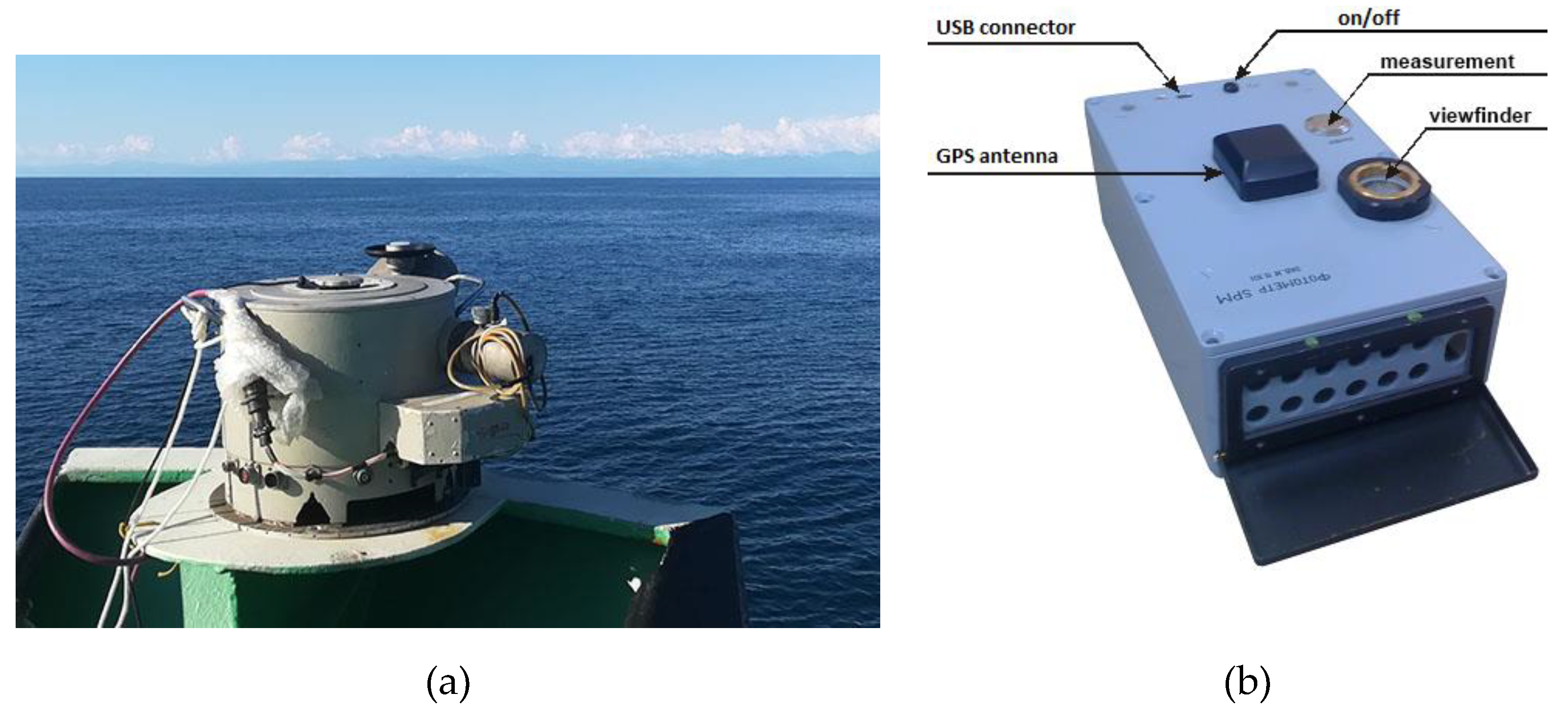
2.2.1. Upwelling Radiation Hyperspectral Measurements

The water-leaving radiance (i.e., upwelling radiance from the sea to the air) was measured from above the water surface from the board of the vessel; the height of the sensor above water was about 5 m. The sensor was pointed at 30° to nadir. Usually, it is necessary to measure the upwelling radiance Lu and the radiance of the sky reflected by the water surface Lr [26]. In this study, a single spectrometer was used, as described in [27]. The spectral range of the spectrometer was 390–750 nm with 1 nm step; the maximum measurement error does not exceed 3%.
Three consecutive measurements with the same measurement geometry were performed: (i) the total upwelling radiance Lu above the water surface (Figure 2a); (ii) the upwelling radiance Lcuv from the absorbing cuvette filled with water (Figure 2b); (iii) the radiance of the horizontal white Lambertian panel Lp (Figure 2c). The cuvette was of 200 mm × 100 mm length × width and had a ~5 cm layer of water. Its walls and bottom were made of 3 mm neutral dark glass that absorbs >99% of the light [28]. The upwelling underwater radiance was negligible, so, Lcuv ≈ Lr. The radiance of the Lambertian panel Lp with a known reflection coefficient Rp was used to estimate the downwelling radiance Ld as Ld = Lp/Rp. Coefficient Rp was obtained by cross-calibration with Spectralon reflectance standard. This method is consistent with the NASA protocols [29].
Measurements of Lu, Lr and Lp were performed within ~5 min. This short time interval implies that illumination conditions do not change during the measurements. The spectra of Lu, Lr and Lp were smoothed by the median filter. After that, the remote sensing reflectance spectra Rrs were calculated according to [26]:
R r s = L u L r L p R p .
The proposed method was applied in sea expeditions [30,31] (Figure 3a) or from a stationary oceanographic platform [27]. The obtained spectra will be further denoted as in situ spectra.

2.2.2. Atmospheric Measurements

The spectral transparency of the atmosphere was measured with SPM sun photometer [32] (Figure 3b) at eleven wavelengths λ (340, 379, 441, 500, 548, 675, 872, 1020, 1244, 1556 and 2134 nm). These measurements are used to calculate the spectral AOD τ λ α , the parameters α, β of the Ångström formula τ λ α = β · λ α , optical depth of coarse- ( τ c ) and fine-mode aerosol τ 500 f = τ 500 a τ c for the wavelength of 500 nm. Methods and algorithms for calculating these characteristics were presented in [32,33].
The SPM sun photometer is a portable instrument for measuring the spectral transparency in the “transparency windows” of the atmosphere (wavelength ranges that lie outside the main intervals of absorption of atmospheric gases) and the absorption band of water vapor (940 nm). Data processing (calculation of physical characteristics) is performed using a special computer program.
The SPM photometer receives direct radiation from the Sun as it passes through the Earth’s atmosphere. In order to obtain aerosol optical depth due to scattering, molecular scattering and absorption are excluded from the signal. Earlier (from 2006 to 2015), similar measurements were carried out for the Black Sea region using the CE-318 photometer within the framework of the AERONET international program. Since 2015 the work under this program has been suspended and photometric measurements have been continued by SPM. Based on research results [34,35], SPM measurements are in good agreement with the data of CE-318 photometer, however, the methods for determining τ λ α , τc and τ 0.5 f for the CE-318 and SPM photometers differ [36,37]. As follows from the comparison of joint measurements with these photometers, the mean square of the deviation between the results ( τ λ α , τc and τ 0.5 f ) does not exceed the error of their measurements. AOD by SPM in the spectral range of 340–2134 nm is provided with an error not exceeding 0.01.

2.3. Satellite Data

Satellite data from MODIS/Aqua, MODIS/Terra, OLCI/S3A, and OLCI/S3B Level 2 obtained from Oceancolor Web [38] and Copernicus [39] websites, were used in this study. The time and coordinates of satellite acquisition coincided with the time and coordinates of field measurements within 3 h and 1 km. Data were processed using the SNAP software package. Only the pixels with no STRAY LIGHT flag were considered.
We used standard satellite inversion products such as Rrs in 10 optical channels for MODIS (412, 443, 469, 488, 531, 547, 555, 645, 667 and 678 nm), 11 channels for OLCI (400, 412, 442, 490, 510, 560, 620, 665, 673, 681 and 709 nm). MODIS Level 2 Rrs was multiplied by π to obtain dimensionless quantities as measured in situ. MODIS also provides the Angstrom parameters and atmosphere aerosol optical depth at 869 nm that were compared to the same quantities obtained from surface measurements.

2.4. Standard Atmospheric Correction Performance

The hyperspectral in situ data R r s ( λ )   were weighted by the spectral response function S R F ( λ ) of MODIS A/T or OLCI S3A/B [38] and converted into the simulated remote sensing reflectance compatible with satellite bands:
R r s s i m ( λ ) = λ 1 λ 2 S R F ( λ ) R r s ( λ ) d λ λ 1 λ 2 S R F ( λ ) d λ ,
where λ 1 and λ 2 are the border wavelengths of the certain spectral band.
We used these statistical metrics to evaluate the accuracy of standard atmospheric correction:
R M S E = 1 N i = 1 N ( y i y i m ) 2 ,
M A P E = 1 N i = 1 N | y i y i m | y i m · 100 ,
B i a s = 1 N i = 1 N ( y i y i m ) ,
where y i   and y i m   are the predicted and measured values. In this case, predicted values are the Rrs given as the standard satellite product, measured values were those R r s s i m obtained from in situ Rrs collected during the cruises.

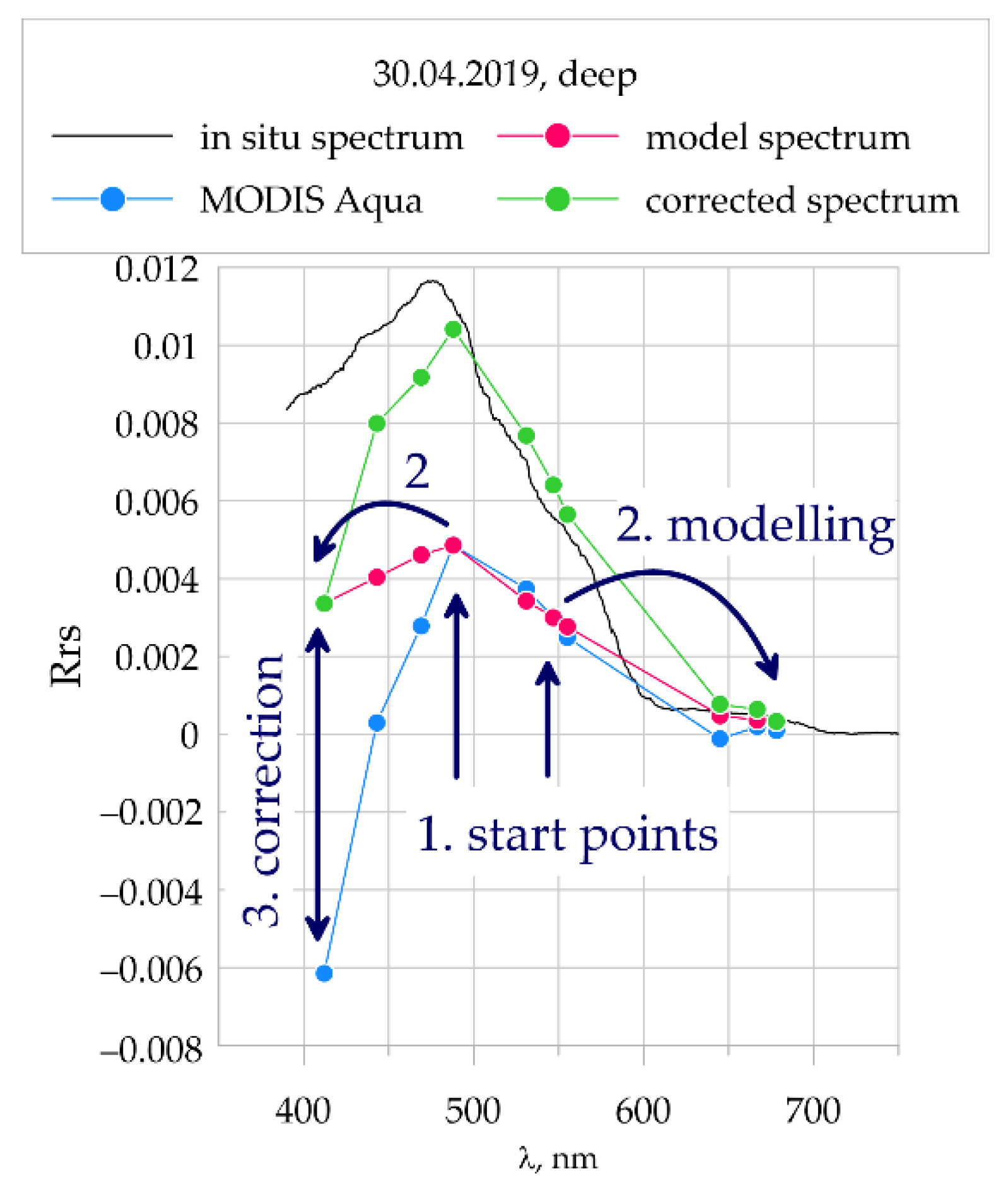
2.5. Additional Correction

We are going to improve Level 2 satellite data R r s ( λ ) by introducing a correctional item   C ( λ ) :
R r s ( λ ) = R r s ( λ ) + C ( λ ) .
It allows for compensating the negative Rrs values which occur in the case of the bad performance of standard atmospheric correction. Spectral dependence of C ( λ ) correspond to spectral dependence of atmospheric correction error. Its spectral behavior was determined earlier by approximating 1st eigenvector of upwelling radiances at the top of the atmosphere [40]. In the general case, it is given as:
C ( λ ) = X λ ν + Y ,
where X and Y are found for each Rrs spectrum from the system of equations
{ C ( λ v i o ) = R r s ( λ v i o ) R r s ( λ v i o ) = X λ v i o ν + Y , C ( λ r e d ) = R r s ( λ r e d ) R r s ( λ r e d ) = X λ r e d ν + Y ,
where λ v i o and λ r e d are wavelengths at the ends of the measurement range, for example, for MODIS λ v i o = 412 nm and λ r e d = 678 nm; R r s ( λ v i o ) and R r s ( λ r e d ) are the measured values.
From system (8), we get:
X = C ( λ r e d ) C ( λ v i o ) λ r e d ν λ v i o ν ,
Y = C ( λ r e d ) X λ r e d ν .
The calculation of R r s ( λ v i o ) and R r s ( λ r e d ) is based on a two-parametric reflectance model similar to the GSM model [41], since we are only interested in bands at the ends of measurement range, and do not consider bands of chlorophyll-a absorption. It is a valid assumption for the Black Sea waters, where the optical properties are mainly affected by suspended sediments and CDOM, like Case 2 waters.
R r s ( λ ) = k b b w ( λ ) + B λ 0 λ a w ( λ ) + A e S ( λ λ 0 ) ,
where a w ( λ ) and b b w ( λ ) are the absorption and backscattering of pure sea water [42], S is the spectral slope of CDOM absorption, k = 0.15 [27], λ 0   is arbitrary wavelength, in this case 390 nm, B and A are the model parameters. These parameters are supposed to be a backscattering of suspended sediments and nonliving organic absorption at wavelength λ 0 , but since the reflectance model is used here as a mathematical construct, not as a real physical model, they do not have any physical interpretation.
It should be noted that the spectral slope S = 0.012 nm−1 used in this model is lower than 0.017 nm−1, which is characteristic for the sum of the Black Sea CDOM and non-algal particles absorption in the spring season [43]. This is required in order to artificially raise CDOM absorption and to compensate for the missing chlorophyll-a absorption. Value of S = 0.012 nm−1 was obtained by summing up the chlorophyll-a absorption with average spring concentration 0.56 mg/m3 [43] and specific absorption [44], and CDOM and non-algal particles absorption from [43] and approximating it with an exponential function. In the Black Sea, chlorophyll-a has a rather small contribution to absorption, ~18% at 412 nm, and this is why it can be considered a part of CDOM for model purposes.
We used two measured Rrs values, in range 490–560 nm, to calculate A and B:
A = k ( L 2 + ( L 2 / L 1 ) ( R r s 1 a w 1 / k b b w 1 ) ) R r s 2 a w 2 R r s 2 E 2 ( L 2 / L 1 ) R r s 1 E 1 ,
B = 1 L 1 ( R r s 1 a w 1 + A E 1 k b b w 1 ) ,
where indices 1 and 2 correspond to the chosen wavelengths, L = λ 0 / λ ,   E = e S ( λ λ 0 ) .
Correction procedure consists of the following steps (Figure 4):
  • Starting from two measurements e.g., for MODIS, at 488 and 547 nm, find A and B, using Equations (12) and (13)—arrow 1 in Figure 4;
  • Using Equation (11), find R r s ( λ v i o ) and R r s ( λ r e d ) —arrow 2;
  • Find C ( λ v i o ) and C ( λ r e d ) from Equation (8)—arrow 3;
  • Find X and Y using Equations (9) and (10);
  • Find spectral values C ( λ )   —Equation (7) and after that, R r s ( λ ) —Equation (6).
Figure 4 shows the example of the first iteration of the correction procedure. It can be seen that the corrected spectrum is much closer to the one measured in situ, even though no additional information about in situ Rrs was used. For higher accuracy a few iterations are made, at each iteration substituting R r s ( λ ) by R r s ( λ ) found at the previous iteration. From 5 to 10 iterations are enough to get a stable solution, that is, to obtain the absolute difference between R r s ( 488 ) at current and previous step less than 1 × 10⁻⁵.

3. Results

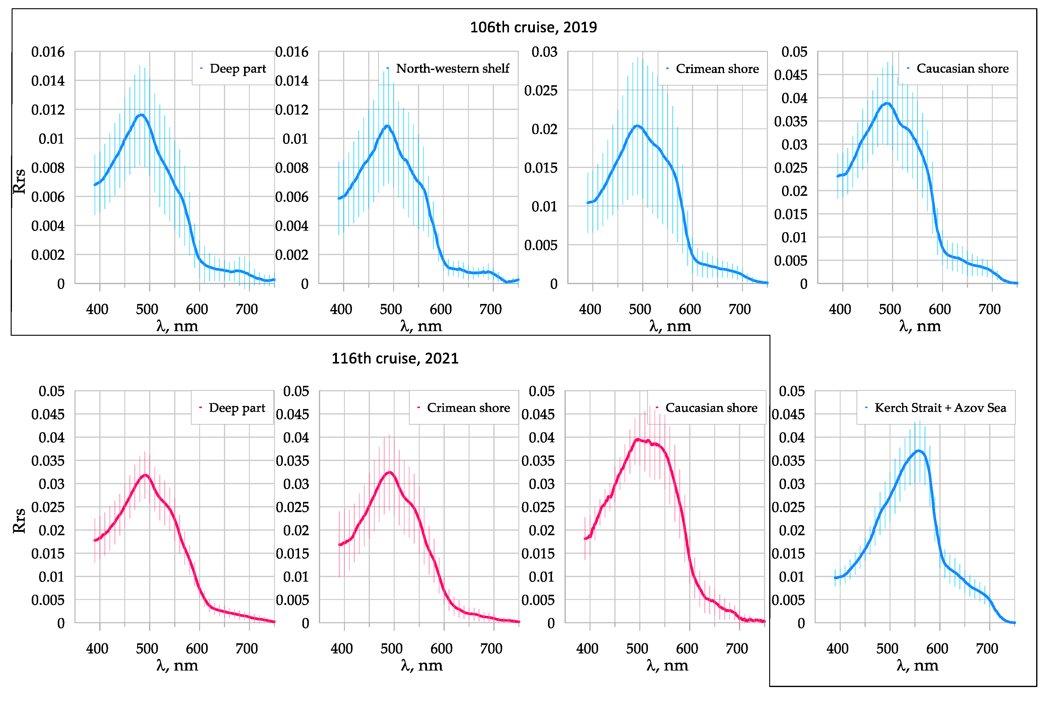
3.1. Reflectance In Situ Spectra

A total of 104 spectra were obtained during the 106th cruise (2019) and 85 spectra during the 116th cruise (2021). All data were divided into two groups—in coastal and shallow waters with depths less than 200 m, and in deep waters. Measurements in coastal and shallow waters show distinct regional differences, so they were subdivided into coastal water of Crimean shore, Caucasian shore, North-western shelf, and the Kerch Strait and the Azov Sea. Reflectance spectra of the Black Sea waters have a characteristic shape that can be characterized by maximum Rrs value and the position of maximum. These data along with the number of measurements N are summarized in Table 1. Rrs spectra are shown in Figure 5. In April–May 2019, according to the field measurements and satellite imagery, the Black Sea waters were much clearer than in the same period of 2018–2021 years.

3.2. Atmospheric Data

In spring–summer of 2019 80 SPM measurements were carried out, and 56—in spring–summer of 2021 (only the days with available satellite observations are counted). The investigation periods include the 106th and the 116th cruises of R/V “Professor Vodyanitsky”, where the measurements were carried out from shipboard simultaneously with Rrs measurements. During March–April 2019 and June–July 2021, measurements were conducted on the oceanographic platform and from small vessels in the coastal zone. We included these measurements in the research because the number of coastal stations with the atmospheric measurements carried out during R/V cruises was not sufficient due to weather conditions. All SPM measurements were performed when the Sun was not covered by clouds.
The obtained data were used to determine daily average values of AOD and parameters α, β of the Angstrom formula τ λ α = β · λ α , which describes the spectral dependence of AOD. The parameters α and β were calculated by the least squares method after taking the logarithm of the wavelength in the range 441–872 nm. Of Angstrom parameters, only parameter α will be considered, since it determines the spectral behavior of AOD and therefore, the atmospheric correction. Table 2 shows statistical characteristics of τ 872 α and α from SPM measurements and τ 869 α and α as a standard MODIS product. In total, 23/23 SPM measurements were compared to MODIS Aqua/Terra data in 2019 and 25/23 in 2021.
The time course of daily averages is shown in Figure 6. It should be noted that despite showing daily averages, the statistics in Table 2 are based on individual measurements that were used for comparison with satellite products. The standard deviation of AOD during the day is usually less than 20%, SD of α is less than 10%. In 2019 and 2021 they do not exceed the standard deviation of mean long-term values [35,45]. A fairly good agreement between the results is observed not only for the average AOD values, but also for their most probable values. Daily variations of in situ AOD and parameter α are shown in Figure 6 as error bars.

3.3. Comparison of Satellite and In Situ Reflectances

All stations were divided into two groups: ‘coastal’, performed near-shore in the shelf zone (depths less than 200 m) and ‘deep-sea’. Measurements in the wide areas of open water with depths of less than 50 m (in Azov Sea and at northwestern shelf) were also compared to satellite data for illustration purposes but excluded from statistical evaluations, because we want to see just how water–land interaction affects the Rrs measurements.
Data for comparison were chosen so that the time difference between satellite acquisition time and in situ measurements was less than 3 h, the coordinate difference was less than 0.01°. We did not take the 3 × 3 pixels average of satellite Rrs, instead we show 3 × 3 pixels variability. In the coastal zone, the spatial variability of bio-optical properties is high, so the coordinate difference can lead to significant discrepancy between the remote sensing and in situ reflectance. This is why the satellite data were checked for spikes, and pixels marked with the STRAY LIGHT flag were excluded. The total amount of stations where a comparison was successfully made, is shown in Table 3.
Figure 7 demonstrates some examples of the mentioned comparison. Both in deep-sea and coastal conditions negative values in short-wave bands can be observed in satellite data. This fact shows how not just stray light can affect the performance of atmospheric correction, but also cloud margins and atmospheric inhomogeneity of other kind.
Variability in satellite data between adjacent pixels is shown in Figure 7 as error bars. Unfortunately, we are unable to show the temporal variability in the in situ data, since the measurements only lasted 5–10 min. We can roughly estimate the maximum variability in the coastal zone, using Rrs measurements on the oceanographic platform in summer 2021 (not published yet). According to our measurements, maximum variability within a day when measuring approximately every hour reached 14.1% at 390 nm, 9.8% at 488 nm and 11.2% at 547 nm.
Figure 8 shows spatial distributions of Rrs(555) by MODIS Aqua/Terra on a typical day of 2019 and 2021 compared to the distributions of in situ Rrs(555) obtained during the cruises. The in situ data were obtained over about 3 weeks, so the map reflects the averaged distribution of optical characteristics and has some time shift. But in general, there is an agreement between in situ and satellite distributions both in the magnitude and in the spatial structure.

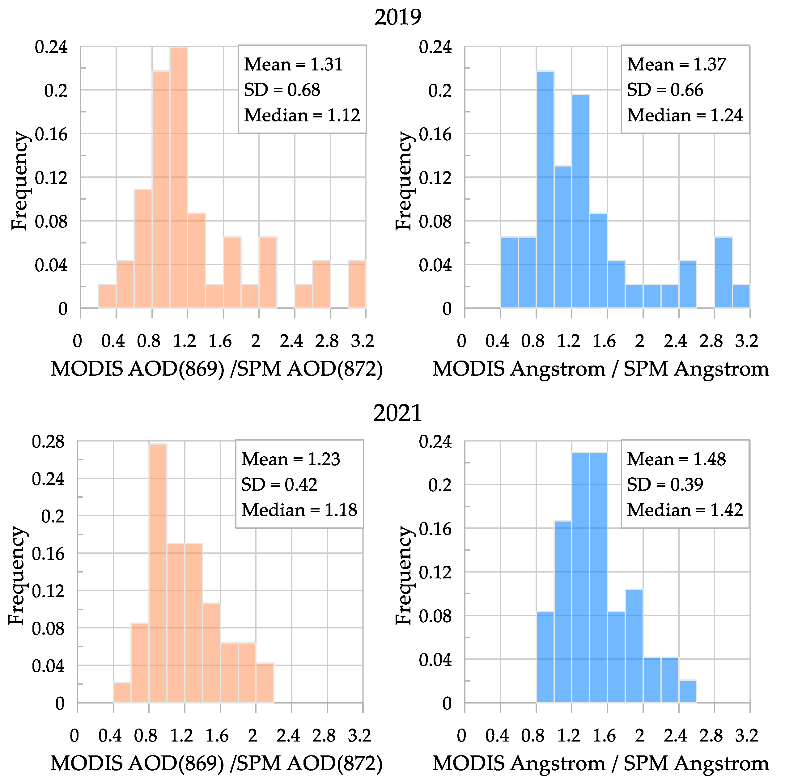
3.4. Comparison of Atmospheric Parameters

To compensate for atmospheric correction errors, we need to know its characteristic features. From Table 2 and Figure 6 we can see that while AOD from satellite and ground-based measurements are rather close, the mean Angstrom parameter differs significantly. In order to estimate this difference, we took the ratios τ M O D I S ( 869 ) / τ S P M ( 872 ) and α M O D I S / α S P M . Figure 9 and Figure 10 show the histograms of these ratios for each year and separately for coastal and deep-sea stations. The distribution is not normal and, for example, in 2019 shows a long ‘tail’. A possible explanation is that, according to the analysis of the expedition logs and satellite imagery [38], percentage of partly cloudy days in all days with measurements during the research period in 2019 was higher than in 2021: ~81% vs. ~67%. The analysis of wind directions, relative humidity and the total amount of cloudiness and precipitation was carried out according to the weather archive [46] for Sevastopol, Feodosia and Anapa (Figure 1) for the periods of research cruises in 2019 and 2021. For all three stations, the wind had predominantly southwestern direction, the percentage of relative humidity for 2019 is 10–20% higher than in 2021, and the total percentage of partly cloudy and precipitation is 15–30% more than in 2021. Partly cloudy conditions allow to perform sun photometer measurements, but general atmospheric heterogeneity is high and can lead to uncertainties in the determination of atmospheric models. The influence of atmospheric conditions on satellite measurements is stronger than on ground-based ones, so this is a possible cause why we observed a larger number of high values in the ratios τ M O D I S ( 869 ) / τ S P M ( 872 ) and α M O D I S / α S P M .
The ‘tail’ in the Angstrom parameter distribution in 2019 (Figure 9) appeared in the distribution for the deep-sea stations (Figure 10). That, again, shows how errors in the determination of aerosol parameters are affected not only by land-water interaction, but also by cloudiness conditions. Examples of cloudiness conditions can be seen in Appendix A.
The most probable values of the Angstrom parameter ratios are higher than 1, a systematic overestimation of α with regard to ground-based measurements is observed. So atmospheric correction term subtracted from the Rrs at the top of the atmosphere is overestimated as well. We assume that errors introduced by atmospheric correction are proportional to AOD, that is, to λ α , since we have no additional information to use. That is why in this study the exponent ν in Equation 6 will be taken equal to mean α = 1.45 . However, in the future, when processing individual measurements, it is possible to use the Angstrom parameter supplied with the Level 2 data.

3.5. Results of Additional Correction

The results of additional correction applied to the coastal and deep-sea data (Figure 11) are shown on the same Rrs spectra that were presented in Figure 7.
The peculiarity of the additional correction algorithm is that if the measured spectrum matches the model assumptions, that is, the changes introduced by the correction are negligible, then it is not corrected. Therefore, no changes occurred for the four spectra from Figure 7, so they are not shown in Figure 11. For those spectra where negative values were observed, they were compensated by the correction item. It should be noted that additional correction reconstructed the shape of the spectra; however, the discrepancies in absolute values are still observed. This could be useful in the cases where absolute values are not needed, for example, when using spectral reflectance ratios or color indices, like NDCI [47].

4. Discussion

4.1. Effect of Additional Correction

To evaluate the amount of discrepancy between in situ and satellite Rrs data, statistical metrics (Equation (3)–(5)) were calculated (Figure 12). In situ Rrs were converted into simulated Rrs (Equation (2)). MODIS Aqua and Terra data gave similar results, so for simplicity all MODIS data were averaged together; same for OLCI.
RMSE shows the obvious result, the discrepancy between the satellite inversion products and the in situ data increases with decreasing wavelength, since the extrapolation error accumulates during the atmospheric correction. Model bias shows the same except for the fact that it is completely negative for coastal stations and mostly negative for deep-sea stations. This means that remote sensing reflectance is systematically underestimated, which is consistent with systematical overestimation of AOD and the Angstrom parameter. Also, Bias for coastal stations is much higher in absolute values, which can be partly explained by high spatial variability of water optical properties in the coastal zone. If coordinate and time match were not accurate enough, in situ and satellite Rrs could describe different water masses. Another possible cause of high Bias in the coastal zone is atmospheric correction.
There are similar discrepancies in the satellite determination of the atmospheric parameters compared to ground-based measurements in the coastal and deep-sea zones. However, a comparison of the Rrs spectra shows that the errors are still higher in the coastal zone. Possibly the problem is in an insufficient amount of atmospheric data in the coastal zone under different atmospheric conditions and further verification is required. The second possibility is the use of satellite data of high spatial resolution, which will allow comparison with field data with higher accuracy and thus reduce this factor of error, making the effect of atmospheric characteristics variability more visible.
MAPE has sharp peaks in the bands where negative and near-zero Rrs values are often observed, and a minimum in the wavelength range 490–550 nm. This is because the relative error will be lower in the bands where Rrs is maximal. However, this suggests that these bands are ‘the most accurate’, so they can be used for further correction of the satellite data based on Level 2 information.
After the additional correction was applied to satellite Rrs, as described in 2.4, all three metrics were calculated again (Figure 13).
All three metrics became smaller in absolute values, which means that the average discrepancy between in situ and additionally corrected Rrs decreased. Spectral behavior of RMSE suggests that now errors due to spatial variability of water optical properties and errors due to the assumption of two-parametric Rrs model have higher influence on it. The main decrease in RMSE occurred in range 400–500 nm, and in range 550–700 nm the values practically did not change. Figure 13 also shows that the corrected spectra become closer to the in situ Rrs in the range 400–500 nm. This makes it possible in the future to obtain more accurate IOPs from satellite data, especially CDOM and Chlorophyll-a optical properties that contribute to Rrs in this spectral range.
MAPE has smaller spikes since Rrs now has no negative values (Figure 13). It is interesting that bias for deep-sea stations almost did not change, while for the coastal stations it decreased significantly.

4.2. Possible Source of Errors in Additional Correction Algorithm

The proposed algorithm uses only algebraic calculations, so the error of the algorithm can be due to incorrect assumptions. It can be associated with the use of a two-parametric reflectance model and its only input parameter S, as well as with the choice of the spectral slope of the correction term, the parameter ν .
In order to assess the validity of the two-parametric model, the RMSE of the approximation of in situ Rrs by three- and two-parametric model (i.e., with and without chlorophyll-a absorption term) were calculated at wavelengths 400, 412, 678, and 709 nm, i.e., in the bands on which the additional correction for MODIS and OLCI is based (Table 4). Three-parametric model used input chlorophyll-a and CDOM parameters from [43,44]. Approximation was carried out by the least squares method without the optimized procedure that takes into account the spectral features of absorption and scattering by seawater components, which we developed earlier and described in [15], since in this case both models are used only as a mathematical rather than a physical description.
In addition, the table shows the error when changing the parameter S. During the development of the model, it was roughly estimated from biological measurements for one season, but its real value can vary, according to the data in [43], from 0.009 to 0.018.
The two-parametric model can describe in situ Rrs with 20.3% error in band 412, which is lower than for the standard atmospheric correction (~50% for the MODIS radiometer and for the deep-sea zone). The error in the bands 678 and 709 nm are the same for three- and two-parametric models, its high values are explained by small values of average Rrs in these bands.
Another source of error is the incorrect estimation of the Angstrom parameter used in Equation (7). According to satellite data, it can vary from 0.66 to 2.0. This change corresponds to a 4% average error in C ( λ ) throughout the visible range. It should be noted that values at the ends of the spectral range are set by the two-parametric reflectance model and not affected by Angstrom parameter error. So, the effect of this error is a slight change in the shape of the corrected Rrs spectrum.
The advantage of additional correction is that in any case it gives positive values at the ends of the measurement range, even if starting values in the range 480–550 nm are negative.
Another advantage is the fact that the additional correction does not use any in situ data, but only the model description of the Rrs for the Black Sea. It provides a future possibility of readjusting the same algorithm to a different Case 2 water body.

5. Conclusions

This work is based on a large array of field data collected in the northeastern part of the Black Sea in the spring of 2019 and 2021. Matching the results of ground-based measurements of the AOD of the atmosphere and the satellite products showed that the discrepancy between them does not depend on the survey point distance from the coast. The Angstrom parameter from satellite measurements turned out to be overestimated by about 50% on average for both coastal and deep-sea stations.
At the same time, a comparison of the in situ and satellite measurements of Rrs revealed that the errors in determining Rrs are significantly higher in the coastal zone. This difference can be explained by the insufficient sampling of atmospheric data since cloudiness does not limit the measurement of Rrs as much as for atmospheric parameters. Another possible explanation is the high spatial variability of water optical properties in the coastal zone.
The proposed method for additional correction of Level 2 satellite Rrs data is based on the model description of the optical properties of the Black Sea waters and does not use any current state in situ information. It allows compensation for negative Rrs values and significantly reduces the error in retrieving the Rrs spectrum, especially in short-wave bands. In the future, this will make it possible to calculate the IOPs more accurately from the Rrs spectra, such as the chlorophyll-a concentration, and so forth. Additional correction can be applied to the other Case 2 water basins by introducing the changes into the Rrs model, on which it is based.

Author Contributions

Conceptualization, E.N.K. and D.V.K.; methodology, E.N.K.; formal analysis, E.N.K. and D.V.K.; investigation, E.N.K. and D.V.K.; data curation, E.N.K. and D.V.K.; writing—original draft preparation, E.N.K.; writing—review and editing, E.N.K. and D.V.K.; visualization, E.N.K. All authors have read and agreed to the published version of the manuscript.

Funding

This research was carried out within the framework of Russian Federation state task No 0555-2021-0003 “Operational oceanology” and RFBR grant 19-05-50023.

Data Availability Statement

The data presented in this study are available on request from the corresponding author.

Conflicts of Interest

The authors declare no conflict of interest.

Appendix A

Figure A1. Satellite images (MODIS Terra, [38]) of cloudiness conditions over the Black Sea during research cruises in 2019 and 2021. Chlorophyll-a concentration distribution shows the amount of data available for match-up with in situ measurements.
Remotesensing 14 00831 g0a1aRemotesensing 14 00831 g0a1bRemotesensing 14 00831 g0a1c

References

  1. Lee, Z.; Marra, J.; Perry, M.J.; Kahru, M. Estimating oceanic primary productivity from ocean color remote sensing: A strategic assessment. J. Mar. Syst. 2015, 149, 50–59. [Google Scholar] [CrossRef]
  2. Karalli, P.G.; Glukhovets, D.I. Retrieving optical characteristics of the Russian Arctic seas water surface layer from shipboard and satellite data. Mod. Probl. Remote Sens. Earth Space 2020, 17, 191–202. [Google Scholar] [CrossRef]
  3. Gordon, H.R.; Wang, M. Retrieval of water-leaving radiance and aerosol optical thickness over the oceans with SeaWiFS: A preliminary algorithm. Appl. Opt. 1994, 33, 443–452. [Google Scholar] [CrossRef]
  4. Ahmad, Z.; Franz, B.; McClain, C.; Kwiatkowska, E.; Werdell, J.; Shettle, E.; Holben, B. New aerosol models for the retrieval of aerosol optical thickness and normalized water-leaving radiances from the SeaWiFS and MODIS sensors over coastal regions and Open Oceans. Appl. Opt. 2010, 49, 5545–5560. [Google Scholar] [CrossRef]
  5. Wang, M.; Gordon, H.R. A Simple, Moderately Accurate, Atmospheric Correction Algorithm for Seawifs. Remote Sens. Environ. 1994, 50, 231–239. [Google Scholar] [CrossRef]
  6. Mobley, C.; Werdell, J.; Franz, B.; Ahmad, Z.; Bailey, S. Atmospheric Correction for Satellite Ocean Color Radiometry. Available online: https://oceancolor.gsfc.nasa.gov/docs/technical/NASA-TM-2016-217551.pdf (accessed on 25 December 2021).
  7. Lee, S.J.; Ahn, M.-H.; Chung, S.-R. Atmospheric Profile Retrieval Algorithm for Next Generation Geostationary Satellite of Korea and Its Application to the Advanced Himawari Imager. Remote Sens. 2017, 9, 1294. [Google Scholar] [CrossRef] [Green Version]
  8. Moses, W.J.; Sterckx, S.; Montes, M.J.; De Keukelaere, L.; Knaeps, E. Atmospheric correction for inland waters. In Bio-Optical Modeling and Remote Sensing of Inland Waters; Elsevier: Amsterdam, The Netherlands, 2017; pp. 69–100. [Google Scholar] [CrossRef]
  9. Giardino, C.; Brando, V.E.; Gege, P.C.; Pinnel, N.; Hochberg, E.; Knaeps, E.; Reusen, I.; Doerffer, R.; Bresciani, M.; Braga, F.; et al. Imaging Spectrometry of Inland and Coastal Waters: State of the Art, Achievements and Perspectives. Surv. Geophys. 2019, 40, 401–429. [Google Scholar] [CrossRef] [Green Version]
  10. Karabashev, G.S.; Evdoshenko, M.A. The wavelength of satellite reflectance maximum as a remote indicator of water exchange between ecologically different aquatic areas. Oceanology 2015, 55, 327–338. [Google Scholar] [CrossRef]
  11. Afonin, S.V.; Solomatov, D.V. Solution of problems of atmospheric correction of satellite IR measurements accounting for optical-meteorological state of the atmosphere. Atmos. Ocean. Opt. 2008, 21, 125–131. [Google Scholar]
  12. Santer, R.; Schmechtig, C. Adjacency effects of water surfaces: Primary scattering approximation and sensitivity study. Appl. Opt. 2000, 39, 361–375. [Google Scholar] [CrossRef]
  13. Wang, T.; Du, L.; Yi, W.; Hong, J.; Zhang, L.; Zheng, J.; Li, C.; Ma, X.; Zhang, D.; Fang, W.; et al. An adaptive atmospheric correction algorithm for the effective adjacency effect correction of submeter-scale spatial resolution optical satellite images: Application to a WorldView-3 panchromatic image. Remote Sens. Environ. 2021, 259, 112412. [Google Scholar] [CrossRef]
  14. Ueda, S.; Miura, K.; Kawata, R.; Furutani, H.; Uematsu, M.; Omori, Y.; Tanimoto, H. Number–size distribution of aerosol particles and new particle formation events in tropical and subtropical Pacific Oceans. Atmos. Environ. 2016, 142, 324–339. [Google Scholar] [CrossRef] [Green Version]
  15. Mordas, G.; Plauškaitė, K.; Prokopčiuk, N.; Dudoitis, V.; Bozzetti, C.; Ulevicius, V. Observation of new particle formation on Curonian Spit located between continental Europe and Scandinavia. J. Aerosol Sci. 2016, 97, 38–55. [Google Scholar] [CrossRef]
  16. Kalinskaya, D.V.; Papkova, A.S. Optical characteristics of atmospheric aerosol from satellite and photometric measurements at the dust transfers dates. In Proceedings of the SPIE 26th International Symposium on Atmospheric and Ocean Optics, Atmospheric Physics, Moskow, Russia, 12 November 2020; p. 115603S. [Google Scholar] [CrossRef]
  17. Varenik, A.V.; Kalinskaya, D.V. The Effect of Dust Transport on the Concentration of Chlorophyll-A in the Surface Layer of the Black Sea. Appl. Sci. 2021, 11, 4692. [Google Scholar] [CrossRef]
  18. Zhang, M.; Hu, C.; Barnes, B.B. Performance of POLYMER Atmospheric Correction of Ocean Color Imagery in the Presence of Absorbing Aerosols. IEEE Trans. Geosci. Remote Sens. 2019, 57, 6666–6674. [Google Scholar] [CrossRef]
  19. Song, Z.; He, X.; Bai, Y.; Wang, D.; Hao, Z.; Gong, F.; Zhu, Q. Changes and Predictions of Vertical Distributions of Global Light-Absorbing Aerosols Based on CALIPSO Observation. Remote Sens. 2020, 12, 3014. [Google Scholar] [CrossRef]
  20. Kokhanovsky, A.A.; Breon, F.-M.; Cacciari, A.; Carboni, E.; Diner, D.; Di Nicolantio, W.; Grainger, R.G.; Grey, W.M.F.; Höller, R.; Lee, K.-H.; et al. Aerosol remote sensing over land: A comparison of satellite retrievals using different algorithms and instruments. Atmos. Res. 2007, 85, 372394. [Google Scholar] [CrossRef]
  21. Pokazeev, K.; Sovga, E.; Chaplina, T. General Oceanographic Characteristics of the Black Sea. In Pollution in the Black Sea; Springer Oceanography; Springer: Cham, Switzerland, 2021; pp. 55–63. [Google Scholar] [CrossRef]
  22. Kopelevich, O.V.; Sahling, I.V.; Vazyulya, S.V.; Glukhovets, D.I.; Sheberstov, S.V.; Burenkov, V.I.; Karalli, P.G.; Yushmanova, A.V. Electronic Atlas. Bio-Optical Characteristics of the Seas, Surrounding the Western Part of Russia, from Data of the Satellite Ocean Color Scanners of 1998–2018. Available online: http://optics.ocean.ru/ (accessed on 25 December 2021).
  23. Solonenko, M.G.; Mobley, C.D. Inherent optical properties of Jerlov water types. Appl. Opt. 2015, 54, 5392. [Google Scholar] [CrossRef]
  24. Morel, A.; Prieur, L. Analysis of variations in ocean color. Limnol. Oceanogr. 1977, 22, 709–722. [Google Scholar] [CrossRef]
  25. Yunev, O.; Carstensen, J.; Stelmakh, L.; Belokopytov, V.; Suslin, V. Reconsideration of the phytoplankton seasonality in the open Black Sea. L&O Lett. 2020, 6, 51–59. [Google Scholar] [CrossRef]
  26. Mobley, C.D. Estimation of the remote sensing reflectance from above–water methods. Appl. Opt. 1999, 38, 7442–7455. [Google Scholar] [CrossRef] [PubMed]
  27. Lee, M.E.; Shybanov, E.B.; Korchemkina, E.N.; Martynov, O.V. Retrieval of concentrations of seawater natural components from reflectance spectrum. In Proceedings of the SPIE 22nd International Symposium on Atmospheric and Ocean Optics: Atmospheric Physics, Tomsk, Russia, 29 November 2016; p. 100352Y. [Google Scholar] [CrossRef]
  28. Coloured Optical Glass. Specifications. Available online: https://docs.cntd.ru/document/1200023782 (accessed on 28 January 2022).
  29. Mueller, J.L.; Pietras, C.; Hooker, S.B.; Austin, R.W.; Miller, M.; Knobelspiesse, K.D.; Frouin, R.; Holben, B.; Voss, K. Ocean Optics Protocols for Satellite Ocean Color Sensor Validation, Revision 4, Volume II: Instrument Specifications, Characterization and Calibration; NASA’s Goddard Space Flight Center: Greenbelt, MD, USA, 2003; pp. 1–63. [CrossRef]
  30. Karalli, P.G.; Kopelevich, O.V.; Sahling, I.V.; Sheberstov, S.V.; Pautova, L.V.; Silkin, V.A. Validation of remote sensing estimates of coccolitophore bloom parameters in the Barents Sea from field measurements. Fundam. Apll. Hydrophys. 2018, 11, 55–63. [Google Scholar] [CrossRef]
  31. Korchemkina, E.N.; Mankovskaya, E.V. Bio-optical properties of Black Sea waters during coccolithophore bloom in July 2017. In Proceedings of the SPIE 25th International Symposium on Atmospheric and Ocean Optics: Atmospheric Physics, Novosibirsk, Russia, 18 December 2019; p. 1120851. [Google Scholar] [CrossRef]
  32. Sakerin, S.M.; Kabanov, D.M.; Rostov, A.P.; Turchinovich, S.A.; Knyazev, V.V. Sun photometers for measuring spectral air transparency in stationary and mobile conditions. Atmos. Ocean. Opt. 2013, 26, 352–356. [Google Scholar] [CrossRef]
  33. Kabanov, D.M.; Veretennikov, V.V.; Voronina, Y.V.; Sakerin, S.M.; Turchinovich, Y.S. Information system for network solar photometers. Atmos. Ocean. Opt. 2009, 22, 121–127. [Google Scholar] [CrossRef]
  34. Firsov, K.M.; Bobrov, E.V. Restoring the aerosol optical depth by ground measurements of SPM photometer. Math. Phys. Comput. Modeling 2014, 2, 57–65. [Google Scholar] [CrossRef]
  35. Kalinskaya, D.V.; Kabanov, D.M.; Latushkin, A.A.; Sakerin, S.M. Atmospheric aerosol optical depth measurements in the Black sea region (2015–2016). Opt. Atmos. Okeana 2017, 30, 489–496, In Russian. [Google Scholar] [CrossRef]
  36. O’Neill, N.T.; Dubovik, O.; Eck, T.F. A modified Angstrom coefficient for the characterization of sub-micron aerosols. Appl. Opt. 2001, 40, 2368–2375. [Google Scholar] [CrossRef] [PubMed]
  37. O’Neill, N.T.; Eck, T.F.; Smirnov, A.; Holben, B.N.; Thulasiraman, S. Spectral discrimination of coarse and fine mode optical depth. J. Geophys. Res. 2003, 108, 4559–4573. [Google Scholar] [CrossRef]
  38. Oceancolor Web. Available online: https://oceancolor.gsfc.nasa.gov/ (accessed on 23 December 2021).
  39. Copernicus Online Data Access. Available online: https://coda.eumetsat.int (accessed on 23 December 2021).
  40. Korchemkina, E.N.; Shybanov, E.B.; Lee, M.E. Improved method of remote sensing retrieval of sea water admixtures concentrations. In Proceedings of the IV International Conference «Current Problems in Optics of Natural Waters», Nizhny Novgorod, Russia, 11–15 September 2007; pp. 171–174. [Google Scholar]
  41. Maritorena, S.; Siegel, D.A.; Peterson, A.R. Optimization of a semianalytical ocean color model for global-scale applications. Appl. Opt. 2002, 41, 2705. [Google Scholar] [CrossRef]
  42. Smith, R.C.; Baker, K.S. Optical properties of the clearest natural waters (200–800 nm). Appl. Opt. 1981, 20, 177–184. [Google Scholar] [CrossRef]
  43. Churilova, T.; Moiseeva, N.; Efimova, T.; Suslin, V.; Krivenko, O.; Zemlianskaia, E. Annual variability in light absorption by particles and colored dissolved organic matter in coastal waters of Crimea (the Black Sea). In Proceedings of the SPIE 23rd International Symposium on Atmospheric and Ocean Optics: Atmospheric Physics, Irkutsk, Russia, 30 November 2017; p. 104664B. [Google Scholar] [CrossRef]
  44. Churilova, T.; Suslin, V.; Krivenko, O.; Efimova, T.; Moiseeva, N.; Mukhanov, V.; Smirnova, L. Light Absorption by Phytoplankton in the Upper Mixed Layer of the Black Sea: Seasonality and Parametrization. Front. Mar. Sci. 2017, 4, 90. [Google Scholar] [CrossRef] [Green Version]
  45. Kalinskaya, D.V.; Papkova, A.S.; Kabanov, D.M. Research of the Aerosol Optical and Microphysical Characteristics of the Atmosphere over the Black Sea Region by the FIRMS System during the Forest Fires in 2018–2019. Phys. Oceanogr. 2020, 27, 514–524. [Google Scholar] [CrossRef]
  46. Pacпиcaниe пoгoды [Weather Schedule]. Available online: https://rp5.ru (accessed on 23 December 2021).
  47. Mishra, S.; Mishra, D.R. Normalized difference chlorophyll index: A novel model for remote estimation of chlorophyll-a concentration in turbid productive waters. Remote Sens. Environ. 2012, 117, 394–406. [Google Scholar] [CrossRef]
Figure 1. Optical stations performed during the two cruises in 2019 and 2021.
Remotesensing 14 00831 g001
Figure 2. Measurement scheme: (a) the total upwelling radiance, (b) the radiance reflected from water surface, and (c) the radiance reflected from white panel.
Remotesensing 14 00831 g002
Figure 3. (a) Spectrometer on board R/V “Professor Vodyanitsky”, (b) SPM sun photometer.
Remotesensing 14 00831 g003
Figure 4. Additional correction scheme.
Remotesensing 14 00831 g004
Figure 5. Average Rrs spectra measured in the Black Sea during two research periods in 2019 and 2021. Dashed areas show SD.
Remotesensing 14 00831 g005
Figure 6. Daily average values of AOD and Ångström parameter for 2019 and 2021. Notations: MA = MODIS Aqua, MT = MODIS Terra, SPM = SPM sun photometer. Error bars represent daily variations of SPM data.
Remotesensing 14 00831 g006
Figure 7. In situ and satellite reflectance spectra for the coastal and deep-sea stations performed in 2019 and 2021. Notations: IS = in situ, MA = MODIS Aqua, MT = MODIS Terra, S3A/B = OLCI Sentinel 3A/B, time is UTC. Error bars represent 3 × 3 pixels variability.
Remotesensing 14 00831 g007
Figure 8. In situ and satellite Rrs(555). Notations: MA = MODIS Aqua, MT = MODIS Terra.
Remotesensing 14 00831 g008
Figure 9. Frequency distributions of atmospheric parameter ratios for research periods in 2019 and 2021.
Remotesensing 14 00831 g009
Figure 10. Frequency distributions of atmospheric parameter ratios for the coastal and deep-sea stations.
Remotesensing 14 00831 g010
Figure 11. In situ and additionally corrected satellite reflectance spectra. Notations: IS = in situ, MA = MODIS Aqua, MT = MODIS Terra, S3A/B = OLCI Sentinel 3A/B, time is UTC.
Remotesensing 14 00831 g011
Figure 12. Spectral distribution of statistical metrics for coastal and deep-sea stations.
Remotesensing 14 00831 g012
Figure 13. Spectral distribution of statistical metrics after additional correction.
Remotesensing 14 00831 g013
Table 1. In situ Rrs data description.
106th Cruise, 2019116th Cruise, 2021
RegionNRrsmaxλmax, nmNρmaxλmax, nm
Deep central part560.012 ± 0.004483 ± 7530.032 ± 0.005491 ± 6
North-western shelf80.011 ± 0.004489 ± 2---
Crimean shore200.021 ± 0.009491 ± 6250.033 ± 0.008492 ± 5
Caucasian shore70.039 ± 0.009486 ± 670.040 ± 0.005496 ± 12
The Kerch Strait + the Azov Sea.130.037±0.006557 ± 4---
Table 2. Statistics of analyzed atmospheric data.
MODIS AquaMODIS TerraSPM
τ 869 α α τ 869 α α τ 872 α α
2019Mean0.0961.470.0881.360.0751.15
SD0.0510.340.0510.400.0300.33
Median0.0911.560.0681.430.0711.20
2021Mean0.1061.490.0931.500.0941.07
SD0.0530.410.0470.340.0570.28
Median0.1021.610.0761.520.0711.11
Table 3. Number of stations used for comparison.
Cruise106th Cruise, 2019116th Cruise, 2021
StationsCoastalDeep-SeaCoastalDeep-Sea
MODIS A/T2029918
OLCI S3A/B16172026
Table 4. RMSE to average in situ Rrs ratio (%) for two- and three-parametric models.
Model3-Parametric2-Parametric
S = 0.017 nm–1S = 0.009 nm–1S = 0.012 nm–1S = 0.018 nm–1
Band, nm
4006.114.116.121.1
4124.715.820.332.7
67884.185.087.388.7
709119.8118.6119.5119.9
Publisher’s Note: MDPI stays neutral with regard to jurisdictional claims in published maps and institutional affiliations.

