Article

AGNet: An Attention-Based Graph Network for Point Cloud Classification and Segmentation

1
College of Information and Computer Engineering, Northeast Forestry University, Harbin 150040, China
2
Baidu Company Ltd., Beijing 100085, China
3
Aerospace Information Research Institute, CAS, Beijing 100094, China
*
Author to whom correspondence should be addressed.
Remote Sens. 2022, 14(4), 1036; https://doi.org/10.3390/rs14041036
Submission received: 27 January 2022 / Revised: 15 February 2022 / Accepted: 16 February 2022 / Published: 21 February 2022

Abstract

:
Classification and segmentation of point clouds have attracted increasing attention in recent years. On the one hand, it is difficult to extract local features with geometric information. On the other hand, how to select more important features correctly also brings challenges to the research. Therefore, the main challenge in classifying and segmenting the point clouds is how to locate the attentional region. To tackle this challenge, we propose a graph-based neural network with an attention pooling strategy (AGNet). In particular, local feature information can be extracted by constructing a topological structure. Compared to existing methods, AGNet can better extract the spatial information with different distances, and the attentional pooling strategy is capable of selecting the most important features of the topological structure. Therefore, our model can aggregate more information to better represent different point cloud features. We conducted extensive experiments on challenging benchmark datasets including ModelNet40 for object classification, as well as ShapeNet Part and S3DIS for segmentation. Both the quantitative and qualitative experiments demonstrated a consistent advantage for the tasks of point set classification and segmentation.

1. Introduction

Point clouds are the most commonly used representations of 3D data due to the rapid iterative upgrading of sensing equipment and are concerned and applied by more and more researchers for their own unique advantage, which can be acquired by remote sensors [1] or other non-contact methods, such as light, acoustics, and LiDAR [2,3]. For example, the unique spatial information of point clouds can make up for the shortcomings of traditional optical remote sensing images [4], and it is useful for remote sensing tasks, such as road segmentation [5,6], 3D city modeling [7], and forestry monitoring [8]. In addition, point clouds are also widely used in many other fields, such as autonomous driving, augmented reality, and robotics.
Point clouds have attracted much interest for their wide application scenarios and huge potential [9,10,11]. Meanwhile, there are many challenging tasks based on them being proposed, and object classification and segmentation are the two most important tasks [12]. Object classification is the basis of object detection, automatic driving, and 3D reconstruction [13]. It plays a key role in many fields, for example face recognition is usually based on an efficient real-time classification algorithm [14]. Point cloud classification, however, is still facing challenges, and more work is urgently needed to solve the current difficulties, which is mainly reflected in the robustness and efficiency that cannot meet the fast-growing needs of industry [15]. Moreover, the particularity of the point cloud data structure also brings huge challenges to the object classification and semantic segmentation task [16]. Usually, the collected point clouds can be divided into three types: object point cloud, indoor scene point cloud, and outdoor scene point cloud. For semantic segmentation tasks, indoor and outdoor scene datasets are usually used to evaluate the performance of networks. The dataset of the outdoor scene puts forward higher requirements for the model due to the larger amount of data, such as Semantic3D [17], Campus3D [18] and SensatUrban [19]. The spatial size and points are usually ten-times or more than that of indoor scene point clouds. All the point clouds have sparseness and replacement invariance [20].
The irregular structure makes it impossible to directly apply traditional image processing methods to point cloud data. The rapid development of deep learning promotes a variety of methods for point cloud processing tasks. These point cloud processing methods based on deep learning have proven their effectiveness with excellent classification results. Some process point clouds by voxeling the space [21]. This leads to much additional memory consumption and computational overhead. Another family of methods processes the point clouds directly. Different from multi-view methods [16] or volumetric methods, PointNet [22] takes the lead in processing the point clouds directly. It applies the shared multi-layer perceptron (MLP) on each point to extract features and aggregate the global features by symmetric functions consistently regardless of the internal order. PointNet, however, cannot effectively extract local features because it handles each point independently. There is no information exchange between different points, but only the transformation of their own features, which leads to the imbalance between global and local features. This problem is improved by the sampling and grouping operations proposed by PointNet++ [23], as shown in Figure 1a.
Benefiting from the successful expansion of graphs and other nonlinear structures in the field of deep learning, graph convolutional networks (GCNs) have received increasing attention in recent years [2]. Inspired by this, the dynamic graph CNN (DGCNN) [24] introduces a new edge convolution to calculate the graph structure dynamically at each network layer and aggregates the features of the central node in the local graph and its corresponding edge features. As shown in Figure 1b, the DGCNN also uses the max-pooling strategy to aggregate the features, which is the same as PointNet++. Even if the DGCNN has extracted local geometric information by connecting edge features and center point features, it still lacks enough local topology. In addition, we can observe that all the methods implement the symmetric function normally by the max-pooling strategy, which is used to aggregate the global feature from the local region. However, the max-pooling strategy can only aggregate the most important features while discarding a large amount of the features that are rich in geometric information. This results in the local information of the point cloud not being completely extracted and used, and more information is simply abandoned directly during the aggregation.
In order to solve the above problems, we used attention pooling to aggregate the features from local neighbors and designed a graph attention module (AGM), as shown in Figure 1c. Based on this module, we propose our graph attention-based network (AGNet) for a variety of 3D analysis tasks including object classification and segmentation. AGNet constructs a local topology by designing a graph-like structure in a local region determined by the k-NN method and applying a novel attention mechanism to aggregate the important local features on point clouds. We used this method to increase the receptive field of each point and enriched the local information of the point cloud by constructing better local geometric features to ensure that each topological structure can better represent the local area it represents. We conducted both quantitative and qualitative experiments including object classification, segmentation, and a series of ablation experiments and achieved a 93.4% accuracy on ModelNet40 [25], 85.4% mIoU on ShapeNet Part [26], and 59.6% mIoU on S3DIS [27]. The key contributions of our work are summarized as follows:
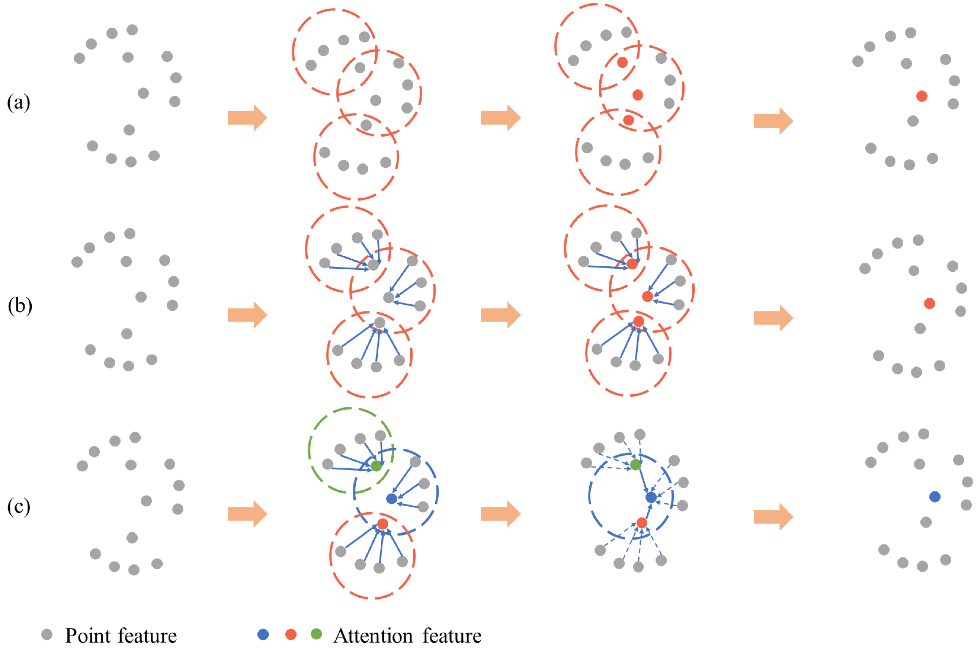
  • We propose a novel feature extraction module based on an attention pooling strategy called AGM, which constructs a topology structure in the local region and aggregates the important features by the novel and effective attention pooling operation;
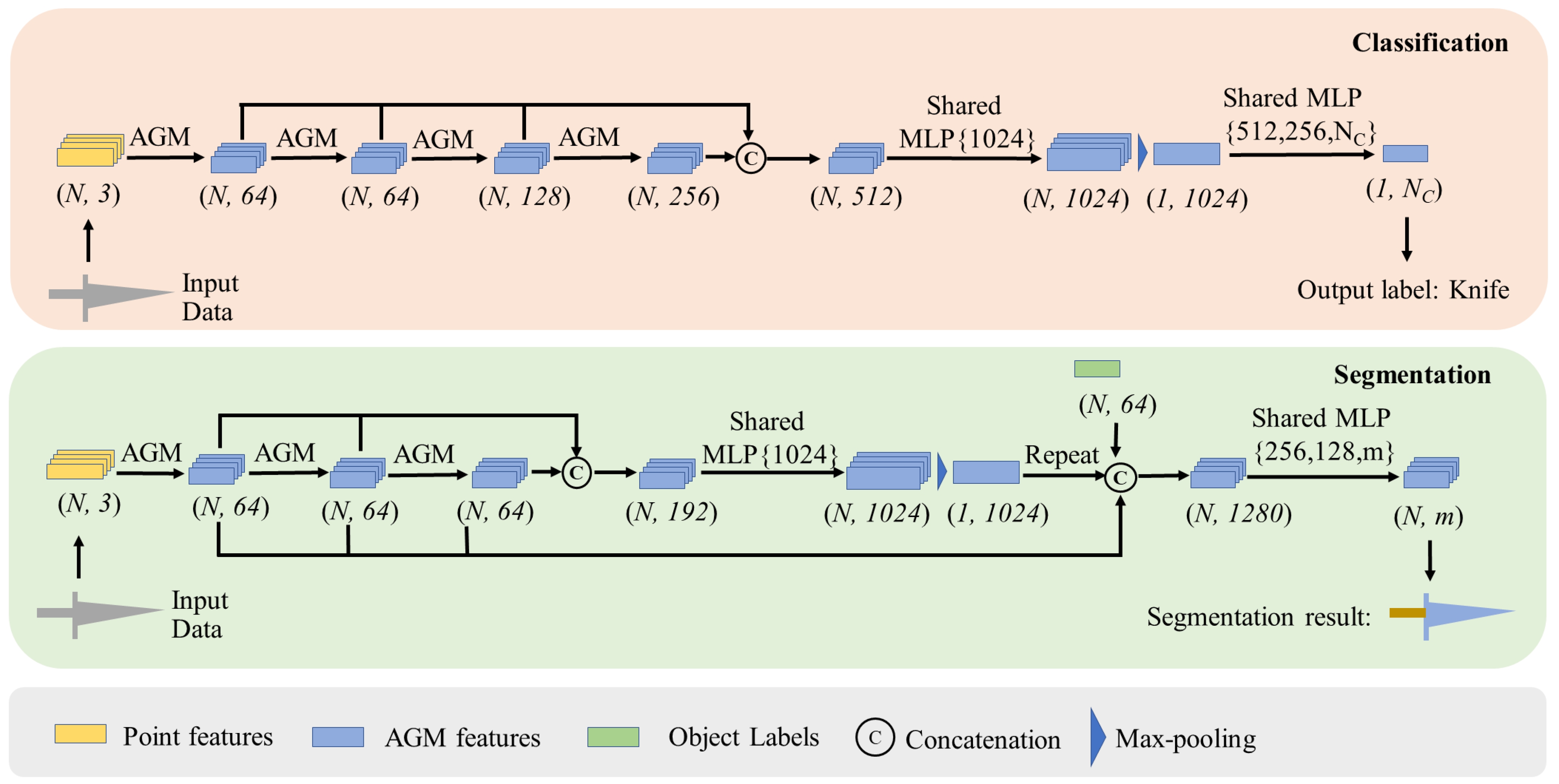
  • We constructed a high-performing network called AGNet based on our attention graph module. The network can be used for point cloud analysis tasks including object classification and segmentation;
  • We conducted extensive experiments and analyses on the benchmark datasets and compared with the current best algorithm, which proved that we achieved results close to the state-of-the-art.

2. Related Work

Traditional algorithms for 3D data usually incorporate geometry estimation and model reconstruction. In recent years, deep-learning-based methods have proven their powerful capabilities in high-dimensional and accurate feature expression on 3D object classification and semantic segmentation [28]. Assisted by deep learning, researchers have focused on data-driven approaches via convolutional neural networks (CNNs) [29]. Point clouds can be defined as a series of unrelated points with three-dimensional coordinates [30]. The sparse and irregular structure of the 3D point clouds is quite different from the 2D image. Therefore, it is difficult to directly transfer the typical 2D image processing method to the 3D point cloud.
To a certain extent, the quality of extracting features determines the accuracy of the result of the point cloud classification task. Therefore, the task of point cloud data classification is to design a module that can better extract point cloud features. Based on this, many methods have emerged in the field of deep learning to extract local and global features of point clouds.

2.1. Projection-Based Methods

Considering the processing methods of 2D images, a straightforward view is to try to migrate the CNN to the processing of 3D point clouds, that is to use the structured operation of convolution to process unstructured point cloud data. An inspiring method is the MVCNN [16], which can project the 3D point cloud in multiple perspectives once to obtain multiple views from different angles and then process these views through the CNN and apply some existing 2D image processing methods to classify the point clouds. Although MVCNN has achieved crucial performance, projecting the point cloud will result in the loss of the spatial geometric information of the point clouds because even multi-angle projection cannot completely cover the geometric information of all angles of the point cloud. For the above reasons, SnapNet-R [31] uses a combination of multiple sets of RGB images and depth images. This method uses multi-view input. The performance is improved compared to the MVCNN, but the generated 3D image still faces the problem of inaccurate boundary classification. In addition, different projection angles will generate different images, which will also have a huge impact on the results of the experiment.

2.2. Voxel-Based Methods

Similar to the view of multi-view processing, another way to apply convolution on the point clouds is to represent the point clouds in voxels instead of using multi-angle projection. In this way, the geometric information in the point cloud space can be retained as much as possible, and the loss of three-dimensional geometric features can be avoided. VoxNet [21] uses voxelization to process point clouds, which significantly improves the accuracy. Due to the unevenness of the point clouds, some locations are very sparse, resulting in a large number of invalid grids during the voxelization process, which is very inefficient. Computing operations will take up much memory and spend much time training. For specific sparse problems, there are some follow-up improvements, such as designing a dedicated sparse convolutional network or sampling first and then calculating. Aiming at the problem of large memory consumption and storage difficulties, researchers use k-d trees, octrees, and other methods for storage. SEGCloud [32] adopts the method of dividing and then processing, which first divides the large-scale point cloud into small sub-point clouds and then uses trilinear interpolation and the conditional random field to process.

2.3. PointNets

The emergence of the PointNet [22] structure has enabled a new processing method for point clouds in the field of deep learning. PointNet directly operates on the original point cloud without formatting preprocessing. Its ability to handle point clouds so easily mainly relies on the symmetric function structure designed by it. Through the insensitivity of the symmetric function to the input data, it avoids the problems caused by the disorder of the point cloud. The PointNet method, however, also has some shortcomings. When extracting features, the max-pooling operation will extract the largest feature value and discard other relatively unimportant features, which will be further magnified, especially in scene segmentation, as an independent object will often be cut into two parts. By gradually expanding the receptive field of the feature map, PointNet++ [23] makes each pixel contain more and more information. Through this method, PointNet++ and a series of subsequent methods can better capture the local information.

2.4. Graph Convolution and Attention Mechanism

The graph convolution neural network and attention mechanism are suitable for dealing with unstructured data. Contrary to the PointNet family, the graph convolution neural network constructs a directed graph structure for each point or sub-point cloud and uses the graph structure for subsequent processing, which is usually determined by the k-NN method. AdaptConv [33] proposes a novel convolution operation with an adaptive kernel, which gives more choices in convolution. Compared with fixed weights, AdaptConv is much more flexible. The 3D-GCN [34] also designs a learnable kernel to capture local information in the convolution operation and shows its strong feature expression ability, which also uses the graph as the input data of the network. The DGCNN [24] applies EdgeConv at all layers to dynamically calculate the graph structures obtained by the k-NN method, which is the same as the above two approaches.
With the great achievements of the attention mechanism in the field of natural language processing [35,36], more and more people have begun to pay attention to it, especially in computer vision [37,38]. The attention mechanism is extremely suitable for point cloud data processing, because it can extract more important features from multiple complex features [2,39]. Based on this, researchers found that the attention mechanism has also achieved gratifying results in the field of point clouds, and even further extended it to Transfromer. GAPNet [39] designs a self-attention model to capture the attention feature with local information. DGANet [2] uses the dilated k-nearest neighbor search algorithm to capture the local information, which can be learned by the attention features. However, we just used the normal k-NN to extract local features directly. The extracted features also include distance information. OE-CNN [40] designs an orientation-encoding module to search in eight directions to realize the effective feature. GACNet [41] proposes an end-to-end network to process structural features and uses a convolution operation dedicated to processing graph structures. LAE-Conv [42] proposes a local attention convolution to aggregate long-range information and captures the global features by the pointwise attention module. Point Transformer [43] proposes a novel method to process point clouds, which is improved by the attention mechanism. These methods prove that the attention mechanism has the same excellent performance in point cloud processing and natural language processing, but most of them still use max-pooling to aggregate neighboring features.

3. Methods

In this work, we introduce a novel network named the attention-based graph network (AGNet), which can better capture the features by constructing a k-NN graph structure and aggregating by the attention mechanism. We introduce this section with the following two parts: the attention graph module and attention pooling.

3.1. Network Architectures

We constructed our classification network with four AGMs, as shown in Figure 2 (top branch). Gradually, four MLP layers are used with the convolution kernels of 64, 64, 128, and 256, respectively. Every new layer uses a new graph, which is based on the features extracted by the AGMs. Dropout layers are used in the last two MLP layers, and we set the dropout rate to 0.5. We set the number k of the k-NN method to 20 for all AGMs in the classification task, which was selected by the ablation experiment. The multi-scale features were extracted and aggregated by shortcut connections and MLP layers with Leaky ReLU and batch normalization, respectively. Finally, the global feature can be aggregated by a global pooling strategy, and 2 MLP layers with kernels of 512 and 256 were used to obtain the class scores.
We extended our network to segmentation tasks. Both part segmentation and semantic segmentation process each point as a single category. As shown in Figure 2 (bottom branch), three MLP layers were used to aggregate the local information. An MLP layer with a kernel of 1024 and global pooling were used respectively to capture the global feature with 1024 dimensions. Then, the global feature repeats N times to connect with the previous features and the object labels. At the end, two MLP layers were used to output the segmentation results.
Different from [44], we still used points as the input instead of 3D voxel grids. The point clouds need to be divided into several 1 m × 1 m blocks first because of their large amount. Besides, each block was sampled to 4096 input points. The later data processing method was completely consistent with the dataset of indoor scenes.

3.2. Attention Graph Module

With the structure shown in Figure 3, the designed AGM takes a set of points with d i n dimensions as the input data and processes the points into d o u t dimensions. Specifically, the AGM constructs a local graph by the k-NN method and applies attention pooling on the aggregated features. The attention pooling module receives the local graph and calculates the attention scores to give different weights to features of different importance.

3.2.1. Attention Graph Convolution

A point cloud with N points can be denoted as a set: P = { p 1 , , p n } , and we set the point cloud to have D dimensions: P R D . Therefore, each point has D-dimensional features, which may also contain additional information including the intensity, color, normal vector, and so on, in addition to the most basic three-dimensional coordinate information p i = ( x i , y i , z i ) . The dimension of features usually changes while passing through the layers of the network, and we generally use D to represent the dimension of the feature given by the previous network layer and use D to represent the dimension of the feature to be output to the next network layer.
Consider a set of points, which can be denoted as a directed graph G = ( V , E ) , where the vertices V = { V i | i = 1 , , n } and edges E V 2 . Obviously, a center point p i naturally has the edge to itself. Specifically, a set of points P R D can be represented by a k-NN graph G, which aggregates the local information. Each edge can be denoted by its neighbors:
k i j = Φ ( p i , p j )
where i ( 1 , n ) , j ( 1 , k ) , and Φ is a set of learnable parameters.
At the end, a feature transformed by an attention graph module is defined as:
p i = Γ i ( 1 , n ) ( Φ ( p i , p j ) ) , j ( 1 , k )
where Φ is the attention pooling to aggregate the local features.
Actually, a point cloud with D dimensions can be processed into D dimensions by the attention graph module. The point cloud P = { p 1 , , p n } aggregates more important local information.
In this paper, we adopted an asymmetric function to represent the local features.
Φ ( p i , p j ) = Φ ( p i , p i , p j 2 , p j p i )
where p i , p j 2 is the distance between p i and p j .
The features that need to be sent to the attention pooling layer aggregate the global information, respectively, which is represented by the coordinates of p i , and the local information, which can be represented as p i , p j 2 and p j p i . It can be defined as:
k i j m = R e L U ( α m · p i + β m · p i , p j 2 + γ m · ( p j p i ) )
p i m = Γ i ( 1 , n ) k i j m
where α 1 , , α m , β 1 , , β m , γ 1 , , γ m are all the learnable parameters.

3.2.2. Attention Pooling

Attention pooling was used to aggregate the set of neighboring point features k i j . The illustration of attention pooling is shown in Figure 4. Existing methods generally use max-pooling to aggregate the neighboring features, and a large amount of the information thus is lost. The attention mechanism can solve this problem well, and we used the attention mechanism to automatically learn the most important features. In fact, the attention pooling mechanism can be defined as follows. Firstly, we computed the attention scores. Given the set of local features k i j = { k i j 1 , , k i j m , , k i j M } , we designed a shared function λ ( ) to learn a unique attention score for each feature. Basically, the function λ ( ) consists of a shared MLP followed by s o f t m a x . It is formally defined as follows:
s i m = λ ( k i j m , ψ )
where ψ is a set of learnable parameters.
The important features can be selected by the scores, which use different weights to represent the features of different importance. As a result, it can be defined as:
k i j ^ = t = 1 T ( k i j m · s i t )
In a word, our AGM can better aggregate the local information of the k neighbors by the k-NN method while processing a point cloud P and give the output informative feature k i j ^ , which determines the dimension of the next layer.

4. Results

4.1. Object Classification

4.1.1. Data

ModelNet40 [25] is a dataset for object classification tasks, which is widely used for point cloud analysis due to its clean shapes and well-constructed data. We evaluated our network on this classical model dataset, consisting of predicting a specific shape never seen before. This dataset also has some defects, such as the uneven division of the training data for the categories. The dataset contains 12,311 meshed CAD models from 40 categories. We preprocessed points in full accordance with PointNet [22]. We used 9843 models for training, and 2468 models were used for testing. Each model was sampled to fit into the unit sphere. We only used the three-dimensional coordinates of the points as the input of the network, which had 1024 points sampled from the mesh, and discarded the original meshes. We randomly rotated, scaled, and jittered the point locations to augment the input points during the procedure of training our network.

4.1.2. Implementation

We implemented our proposed network on the framework of Pytorch and used a single NVIDIA Tesla V100 GPU to train it. We set the k number to 20, which was determined by the results of the ablation experiments later. During the stage of training, we used the SGD algorithm to optimize the model and set the momentum to 0.9 for batch normalization and the minimum learning rate to 0.015 with the learning rate decay scheme of cosine annealing. The batch size was 32, and we used the model with the best result for the overall accuracy from 250 epochs to evaluate the performance of our classification network.

4.1.3. Analysis

Table 1 shows the results of our network for the classification task. Our results are marked in blod. Our network achieved a higher overall accuracy of 93.4%. It was 0.5% better than the DGCNN and made a 4.2% and 2.7% improvement, respectively, compared to PointNet and PointNet++. We kept all the experiments with 1024 point clouds except the last row to ensure consistency with other methods. We further evaluated our network with 2048 points to verify its better performance, and we naturally set k at 40 to make sure it could keep consistency as before. Notably, we actually did not use normal features as inputs, which can significantly improve the performance of our network further, and PointConv and DensePoint use additional features such as normalizing and voting on the points during experiments.
We can also observe from Table 1 that most of the voxel-based methods performed worse than the subsequent graph-based methods. This was due to the limitation of less local information. To tackle this challenge, we designed a graph-based network with an attention mechanism. Our network could better extract local features by constructing a topological structure. What is more, our network consumed less computing resources and occupied less memory than the other methods. Therefore, our network could better capture the local information and achieved a high accuracy in the object classification task compared to the other methods.

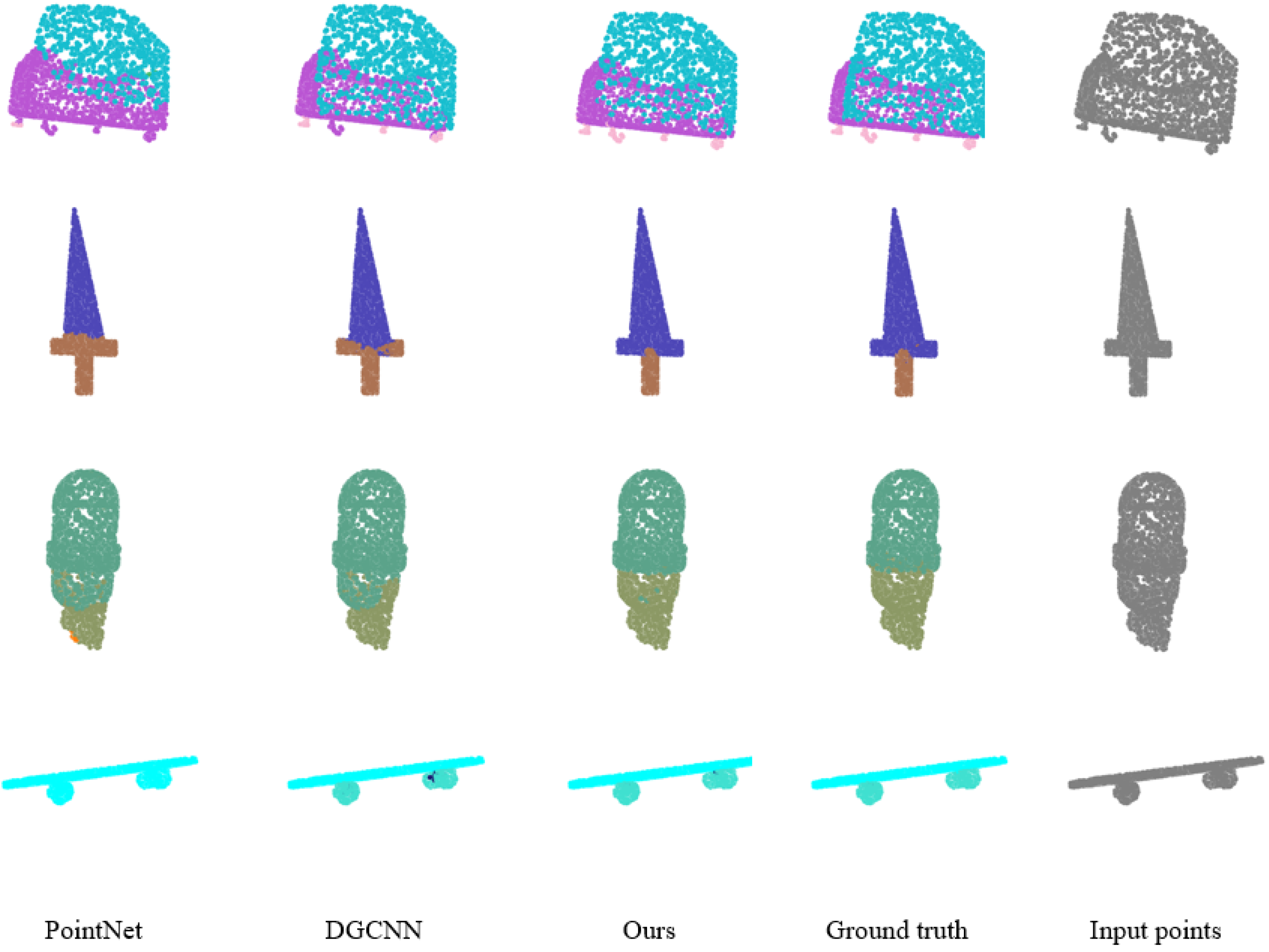
4.2. Shape Part Segmentation

4.2.1. Data

We evaluated our network for 3D object part segmentation on ShapeNet Part [26], which is annotated richly with 2–5 parts for each model and contains 16,880 models that are from 16 shape categories and 50 different parts in total. To ensure a fair comparison with other people’s work, we used the sampled points produced by PointNet [22], which is used widely by most papers. We also split the points with others to be consistent. We used 14,006 models for training and 2874 for testing.

4.2.2. Implementation

We implemented our proposed network on the framework of Pytorch and further extended it to a distributed training scheme to meet the same batch size on two NVIDIA Tesla V100 GPUs. During the stage of training, we also used the SGD algorithm to optimize the model and set the momentum to 0.9 for batch normalization and the minimum learning rate to 0.015 with the learning rate decay scheme of cosine annealing. We still kept the batch size at 32, and we used the epoch with the best result of the accuracy from 200 epochs to test the result of our part segmentation network.

4.2.3. Analysis

We evaluated our network with the category mean intersection-over-union (mIoU) and the instance mIoU and compared the performance with other methods. We evaluated our network with the same scheme as PointNet: We averaged the IoUs of each part of a shape. The IoUs of a category can be computed through the mean value of the IoUs, all of which belong to this category, which can be obtained one by one through the approach above. Finally, we averaged the IoUs of all shapes that were used for testing to obtain the mean IoU. We compared the performance of our network with PointNet, PointNet++, the DGCNN, SO-Net, the PCNN, and some others. The results of the segmentation are in Figure 5. We also visualized the results of our comparison with PointNet and the DGCNN.
Table 2 shows the results of our network for part segmentation. The best results are marked in blod. Our competition results demonstrated that our network can capture the local information, especially compared to those methods with insufficient local information. KPConv also achieved a topperformance due to the fact that it has a novel and effective local feature extraction module.
We compared the results of different methods including PointNet and the DGCNN with our AGNet, and we show the visualization results in Figure 6. In the first row, it is obvious that it was hard to clearly identify the chair legs in the first two columns, which were the results of PointNet and the DGCNN, respectively. Both of them identified the chair legs and the lower half of the chair as a whole. On the contrary, our method could distinguish the chair legs well. In addition, PointNet could not clearly distinguish the back and the surface of the chair due to its lack of local information. From the next two rows, we can observe that our results were more similar to the ground truth, which extracted the complete blade and the appropriately sized lampshade. Both PointNet and the DGCNN could not correctly divide the joint between the blade and the handle into the correct part, nor clearly identify the transition part between the lamp shade and lamp body. The segmentation results of the skateboard in the last row demonstrate the effectiveness of our attention pooling module. We can observe that there were wrong points in the wheel on the right side of the DGCNN, which was mainly caused by its max-pooling strategy. Different from the DGCNN, we used attention pooling to capture the most important feature from the local k-NN graph, and the correct segmentation results were obtained. As a result, a sufficient comparison of the visualization results demonstrated that our network was capable of extracting local features.

4.3. Semantic Segmentation

4.3.1. Data

In order to further verify the effect of our model, we evaluated our proposed network for a more challenging semantic scene segmentation task on the Stanford Large-Scale 3D Indoor Space Dataset (S3DIS) [27], which includes six indoor areas. It contains two-hundred seventy-nine million points that are scanned from two-hundred seventy-one rooms in three different buildings. All points are labeled by semantic level as 13 categories in total, including board, chair, and some other common things. We were consistent with the data processing in [22], where the rooms were divided into blocks with a size of 1 m × 1 m. We used the nine-dimensional vector (XYZ, RGB, and normalized coordinates) to represent a point cloud.

4.3.2. Implementation

We followed our setting of the part segmentation task and randomly sampled 4096 points from each block along with the model being trained. In addition, points used for testing were not sampled. Six-fold cross-validation over the six areas was used, and we evaluated our model with the average results. We followed the same augmentations of random scaling, rotating, and jittering the points.

4.3.3. Analysis

The best results are marked in blod. The results on S3DIS are reported in Table 3, and we compared our results with PointNet and the DGCNN. It is worth noting that KPConv processes point clouds as voxel grids instead of sampling them from blocks. This led to a surge in the number of point clouds used, which was almost ten-times more than ours in their actual implementations. This resulted in additional memory usage and computational overhead, although it could better extract the characteristics of the point cloud and obtain a higher mIoU.
The semantic segmentation results on the S3DIS dataset are shown as Figure 7. Through the visualization results, we can intuitively find that our model could segment some close objects better than PointNet and the DGCNN. Through the first row and third row, we can observe that PointNet and the DGCNN often misclassified objects such as chairs and trash cans with surrounding things, resulting in classification errors, and our model could better distinguish them and classify them correctly. In addition, through the remaining rows, we can find that our model also had better performance in the point clouds with a regular overall shape, such as walls, which is reflected in that it could extract neater and clearer boundaries.

5. Discussion

We also conducted additional ablation experiments on the ModelNet40 [25] dataset, in addition to the above three target classification and segmentation tasks, to explore the specific impact of the different use of some important hyper-parameters during the experiment on our model, such as the number of nearest neighbors used in the graph structure. In addition, we verified the robustness of our model and analyzed the verification results. Finally, by comparing our model with other competitive methods, we proved that our network achieved the best balance between accuracy and complexity.
Different number of k: The results on ModelNet40 are shown as Table 4. We selected some specific representative numbers of nearest neighbors from small to large. We did not test all possible k because after these numbers of nearest neighbors were tested, we could easily find that there was an obvious positive correlation between the accuracy of the model and the number of nearest neighbors when k was small; however, with the increase of k, that is after more than 20, the mean accuracy and overall accuracy of our model would not continue to increase. In fact, with the increase of k, the accuracy of the model would further decline. Our network achieved the highest mean accuracy of 90.7% and 93.4% on the overall accuracy when k = 20 and we marked the results in blod.
We can observe from the results that the number of nearest neighbors had an upper bound. Before reaching this upper bound, the value of k should be increased as much as possible to ensure that the features of surrounding points can be obtained as much as possible. In addition, through the comparison results, we can also easily see that the number of nearest neighbors was not a natter of bigger is better, but related to the density of the input points. By combining the experiment of 2048 input points with the object classification experiment, we can naturally come to the conclusion that the best value of k should be positively correlated with the density of the input points, so as to prevent the results from becoming worse by adding the characteristics of many unnecessary points to the graph-like structure when the input density is small.
In conclusion, we found that the accuracy of the model increased with the increase of the k number, and there was an upper bound. Therefore, we tried our best to select the k corresponding to the maximum accuracy before it dropped.
Robustness test: In addition, we verified the robustness of our model by using the classification network with k = 20. We gradually reduced the number of input points step by step from 1024 to 512, 256, and at last only 128 points input into the model, which was trained in the same way as the object classification part. Figure 8 shows the overall accuracy and mean class accuracy results of the experiment with different numbers of input points. It is obvious that our model achieved a considerable overall performance with 1024 points, and even if the data were reduced to half of the original, which was only 512 points, the model still performed well, which proved the robustness of our model. It is worth noting that if we continued to reduce the input points by the same proportion, the accuracy of our model would decline sharply and could not maintain good robustness. This is because the k value set by our model was 20, that is, for each input point to be predicted, we would find its nearest 20 neighbor points. While there were too few input points, the model could not extract the corresponding graph-like features through the k-nearest neighbor algorithm, which led to the model being unable to find a good topology to characterize the main features of the shape. Accordingly, if the extracted graph structure had a low effect, even if the attention pooling strategy was used, the more important feature could not be extracted from a large number of invalid features.
Complexity analysis: Finally, we compared the complexity of our model to other methods by the number of parameters on the ModelNet40 [25] dataset, and Table 5 shows the results. We can observe that KPConv had a large number of parameters because of its huge calculation, and PointNet had the lowest accuracy.
Compared to PointNet, KPConv, and InterpCNN, the number of parameters of our method was obviously fewer because we used fewer convolution operations and smaller feature dimensions. However, we achieved a higher accuracy of 93.4%. Besides, PointNet++ and DGCNN have fewer parameters than ours, but their accuracy was lower than ours. In addition, MVTN is more than half as large as our model, although its accuracy was 0.4% higher than ours. Therefore, our model achieved the best balance between spatial complexity and accuracy.
Moreover, we compared the processing time of the different algorithms. For a fair experimental comparison, we evaluated these methods on a single RTX 2080 GPU. The results are shown as Table 5. PointNet and PointNet++ had less processing time because both of them only use MLP to extract features. Compared to them, the DGCNN and our model had similar k-NN search operations. Therefore, DGCNN and ours had a similar processing time. However, because the attention pooling strategy took more time, our processing time was somewhat longer than the DGCNN, but it achieved a higher accuracy. Actually, MVTN achieved the best balance between processing time and accuracy. Compared to MVTN, our method cost more time, but the accuracy was lower because of the limitation of the k-NN algorithm, and when the k number increased, the time consumed by the algorithm further increased.

6. Conclusions

In this work, we introduced a novel network on 3D point cloud tasks, called AGNet, which is effective for learning on unstructured data point clouds. The attention mechanism and graph structure are perhaps more suitable for point cloud processing than when they are used for natural language processing or image analysis due to their strong capabilities of extracting local geometric features. By using attention pooling, AGNet can better aggregate the best features from a set of points that is chosen by the k nearest neighbors. We showed the performance on both object classification and segmentation tasks by conducting experiments and evaluating our network on challenging benchmarks such as ModelNet40 with a 93.4% overall accuracy, ShapeNet Part with an 85.2% mIoU, and S3DIS with a 59.6% mIoU. Moreover, we provided ablation studies that demonstrated the feature extraction capabilities of the AGM.
To this end, we would like to try to combine hyperspectral remote sensing images and point clouds. AGNet can better utilize the rich spectral information of two-dimensional hyperspectral remote sensing images while retaining the three-dimensional coordinate information, which is very advantageous when performing semantic segmentation. In addition, AGNet has already achieved considerable capabilities on benchmarks, comparable with the images; however, the point cloud datasets that can be easily obtained are still extremely limited. In the future, we would like to extend our work to larger datasets and merge the different types of data.

Author Contributions

Conceptualization, W.J. and W.Z.; methodology, W.J., G.C. and W.Z.; resources, W.J.; writing—original draft preparation, W.Z. and D.D.; writing—review and editing, W.J., W.Z., L.L., D.D., J.W. and G.C.; visualization, J.W. and L.L. All authors have read and agreed to the published version of the manuscript.

Funding

This research was funded by The Innovation Foundation for Doctoral Program of Forestry Engineering of Northeast Forestry University (4111410203), the National Natural Science Foundation of China (32171777), the Fundamental Research Funds for the Central Universities (2572017PZ04), and the Heilongjiang Province Applied Technology Research and Development Program Major Project (GA20A301).

Institutional Review Board Statement

Not applicable.

Informed Consent Statement

Not applicable.

Data Availability Statement

Restrictions apply to the availability of these data. The data were obtained from Stanford University and are available https://goo.gl/forms/4SoGp4KtH1jfRqEj2/ (accessed on 10 December 2021) with the permission of Stanford University. Publicly available datasets were analyzed in this study. The datasets can be found here: http://modelnet.cs.princeton.edu/ (accessed on 10 December 2021) and https://www.shapenet.org/ (accessed on 10 December 2021).

Acknowledgments

The authors want to thank Stanford University for providing the experimental datasets.

Conflicts of Interest

The authors declare no conflict of interest.

References

  1. Blais, F. Review of 20 years of range sensor development. J. Electron. Imaging 2004, 13, 231–243. [Google Scholar] [CrossRef]
  2. Wan, J.; Xie, Z.; Xu, Y.; Zeng, Z.; Yuan, D.; Qiu, Q. DGANet: A Dilated Graph Attention-Based Network for Local Feature Extraction on 3D Point Clouds. Remote Sens. 2021, 13, 3484. [Google Scholar] [CrossRef]
  3. Štular, B.; Eichert, S.; Lozić, E. Airborne LiDAR Point Cloud Processing for Archaeology. Pipeline and QGIS Toolbox. Remote Sens. 2021, 13, 3225. [Google Scholar] [CrossRef]
  4. Cai, S.; Xing, Y.; Duanmu, J. Extraction of DBH from Filtering out Low Intensity Point Cloud by Backpack Laser Scanning. For. Eng. 2021, 37, 12–19. [Google Scholar]
  5. Wu, B.; Zhou, X.; Zhao, S.; Yue, X.; Keutzer, K. Squeezesegv2: Improved model structure and unsupervised domain adaptation for road-object segmentation from a LiDAR point cloud. In Proceedings of the 2019 International Conference on Robotics and Automation (ICRA), Montreal, QC, Canada, 20–24 May 2019; pp. 4376–4382. [Google Scholar]
  6. Dewi, C.; Chen, R.C.; Yu, H.; Jiang, X. Robust detection method for improving small traffic sign recognition based on spatial pyramid pooling. J. Ambient. Intell. Humaniz. Comput. 2021, 1–18. [Google Scholar] [CrossRef]
  7. Niemeyer, J.; Rottensteiner, F.; Soergel, U. Contextual classification of LiDAR data and building object detection in urban areas. ISPRS J. Photogramm. Remote Sens. 2014, 87, 152–165. [Google Scholar] [CrossRef]
  8. Reitberger, J.; Schnörr, C.; Krzystek, P.; Stilla, U. 3D segmentation of single trees exploiting full waveform LIDAR data. ISPRS J. Photogramm. Remote Sens. 2009, 64, 561–574. [Google Scholar] [CrossRef]
  9. Qi, C.R.; Liu, W.; Wu, C.; Su, H.; Guibas, L.J. Frustum pointnets for 3d object detection from rgb-d data. In Proceedings of the IEEE Conference on Computer Vision and Pattern Recognition, Salt Lake City, UT, USA, 18–23 June 2018; pp. 918–927. [Google Scholar]
  10. Rusu, R.B.; Marton, Z.C.; Blodow, N.; Dolha, M.; Beetz, M. Towards 3D point cloud based object maps for household environments. Robot. Auton. Syst. 2008, 56, 927–941. [Google Scholar] [CrossRef]
  11. Lin, Y.; Yan, Z.; Huang, H.; Du, D.; Liu, L.; Cui, S.; Han, X. Fpconv: Learning local flattening for point convolution. In Proceedings of the IEEE/CVF Conference on Computer Vision and Pattern Recognition, Seattle, WA, USA, 14–19 June 2020; pp. 4293–4302. [Google Scholar]
  12. Chang, A.X.; Funkhouser, T.; Guibas, L.; Hanrahan, P.; Huang, Q.; Li, Z.; Savarese, S.; Savva, M.; Song, S.; Su, H.; et al. Shapenet: An information-rich 3d model repository. arXiv 2015, arXiv:1512.03012. [Google Scholar]
  13. Dai, A.; Chang, A.X.; Savva, M.; Halber, M.; Funkhouser, T.; Nießner, M. Scannet: Richly-annotated 3d reconstructions of indoor scenes. In Proceedings of the IEEE Conference on Computer Vision and Pattern Recognition, Honolulu, HI, USA, 21–26 July 2017; pp. 5828–5839. [Google Scholar]
  14. Wang, F.; Zhuang, Y.; Zhang, H.; Gu, H. Real-time 3-d semantic scene parsing with LiDAR sensors. IEEE Trans. Cybern. 2020, 1–13. [Google Scholar] [CrossRef]
  15. Hu, Q.; Yang, B.; Xie, L.; Rosa, S.; Guo, Y.; Wang, Z.; Trigoni, N.; Markham, A. Randla-net: Efficient semantic segmentation of large-scale point clouds. In Proceedings of the IEEE/CVF Conference on Computer Vision and Pattern Recognition, Seattle, WA, USA, 13–19 June 2020; pp. 11108–11117. [Google Scholar]
  16. Su, H.; Maji, S.; Kalogerakis, E.; Learned-Miller, E. Multi-view convolutional neural networks for 3d shape recognition. In Proceedings of the IEEE International Conference on Computer Vision, Santiago, Chile, 7–13 December 2015; pp. 945–953. [Google Scholar]
  17. Hackel, T.; Savinov, N.; Ladicky, L.; Wegner, J.D.; Schindler, K.; Pollefeys, M. Semantic3d. net: A new large-scale point cloud classification benchmark. arXiv 2017, arXiv:1704.03847. [Google Scholar]
  18. Li, X.; Li, C.; Tong, Z.; Lim, A.; Yuan, J.; Wu, Y.; Tang, J.; Huang, R. Campus3d: A photogrammetry point cloud benchmark for hierarchical understanding of outdoor scene. In Proceedings of the 28th ACM International Conference on Multimedia, Seattle, WA, USA, 12–16 October 2020; pp. 238–246. [Google Scholar]
  19. Hu, Q.; Yang, B.; Khalid, S.; Xiao, W.; Trigoni, N.; Markham, A. Towards semantic segmentation of urban-scale 3d point clouds: A dataset, benchmarks and challenges. In Proceedings of the IEEE/CVF Conference on Computer Vision and Pattern Recognition, Nashville, TN, USA, 20–25 June 2021; pp. 4977–4987. [Google Scholar]
  20. Guo, Y.; Bennamoun, M.; Sohel, F.; Lu, M.; Wan, J. 3D object recognition in cluttered scenes with local surface features: A survey. IEEE Trans. Pattern Anal. Mach. Intell. 2014, 36, 2270–2287. [Google Scholar] [CrossRef] [PubMed]
  21. Maturana, D.; Scherer, S. Voxnet: A 3d convolutional neural network for real-time object recognition. In Proceedings of the 2015 IEEE/RSJ International Conference on Intelligent Robots and Systems (IROS), Hamburg, Germany, 28 September–3 October 2015; pp. 922–928. [Google Scholar]
  22. Qi, C.R.; Su, H.; Mo, K.; Guibas, L.J. Pointnet: Deep learning on point sets for 3d classification and segmentation. In Proceedings of the IEEE Conference on Computer Vision and Pattern Recognition, Honolulu, HI, USA, 21–26 July 2017; pp. 652–660. [Google Scholar]
  23. Qi, C.R.; Yi, L.; Su, H.; Guibas, L.J. Pointnet++: Deep hierarchical feature learning on point sets in a metric space. arXiv 2017, arXiv:1706.02413. [Google Scholar]
  24. Wang, Y.; Sun, Y.; Liu, Z.; Sarma, S.E.; Bronstein, M.M.; Solomon, J.M. Dynamic graph cnn for learning on point clouds. ACM Trans. Graph. (Tog) 2019, 38, 1–12. [Google Scholar] [CrossRef] [Green Version]
  25. Wu, Z.; Song, S.; Khosla, A.; Yu, F.; Zhang, L.; Tang, X.; Xiao, J. 3d shapenets: A deep representation for volumetric shapes. In Proceedings of the IEEE Conference on Computer Vision and Pattern Recognition, Boston, MA, USA, 7–12 June 2015; pp. 1912–1920. [Google Scholar]
  26. Yi, L.; Kim, V.G.; Ceylan, D.; Shen, I.-C.; Yan, M.; Su, H.; Lu, C.; Huang, Q.; Sheffer, A.; Guibas, L. A scalable active framework for region annotation in 3d shape collections. ACM Trans. Graph. (Tog) 2016, 35, 1–12. [Google Scholar]
  27. Armeni, I.; Sener, O.; Zamir, A.R.; Jiang, H.; Brilakis, I.; Fischer, M.; Savarese, S. 3d semantic parsing of large-scale indoor spaces. In Proceedings of the IEEE Conference on Computer Vision and Pattern Recognition, Las Vegas, NV, USA, 27–30 June 2016; pp. 1534–1543. [Google Scholar]
  28. Xu, Y.; Xie, Z.; Chen, Z.; Xie, M. Measuring the similarity between multipolygons using convex hulls and position graphs. Int. J. Geogr. Inf. Sci. 2021, 35, 847–868. [Google Scholar] [CrossRef]
  29. Dewi, C.; Chen, R.C.; Liu, Y.T.; Jiang, X.; Hartomo, K.D. Yolo V4 for advanced traffic sign recognition with synthetic training data generated by various GAN. IEEE Access 2021, 9, 97228–97242. [Google Scholar] [CrossRef]
  30. Zhang, B.; Ni, H.; Hu, X.; Qi, D. Research on Tree lmage Segmentation Based on U-Net Network. For. Eng. 2021, 37, 67–73. [Google Scholar]
  31. Guerry, J.; Boulch, A.; Le Saux, B.; Moras, J.; Plyer, A.; Filliat, D. Snapnet-r: Consistent 3d multi-view semantic labeling for robotics. In Proceedings of the IEEE International Conference on Computer Vision Workshops, Venice, Italy, 22–29 October 2017; pp. 669–678. [Google Scholar]
  32. Tchapmi, L.; Choy, C.; Armeni, I.; Gwak, J.; Savarese, S. Segcloud: Semantic segmentation of 3d point clouds. In Proceedings of the 2017 International Conference on 3D Vision (3DV), Qingdao, China, 10–12 October 2017; pp. 537–547. [Google Scholar]
  33. Zhou, H.; Feng, Y.; Fang, M.; Wei, M.; Qin, J.; Lu, T. Adaptive Graph Convolution for Point Cloud Analysis. In Proceedings of the IEEE/CVF International Conference on Computer Vision, 19–25 June 2021; pp. 4965–4974. [Google Scholar]
  34. Lin, Z.H.; Huang, S.Y.; Wang, Y.C.F. Convolution in the cloud: Learning deformable kernels in 3d graph convolution networks for point cloud analysis. In Proceedings of the IEEE/CVF Conference on Computer Vision and Pattern Recognition, Seattle, WA, USA, 13–19 June 2020; pp. 1800–1809. [Google Scholar]
  35. Vaswani, A.; Shazeer, N.; Parmar, N.; Uszkoreit, J.; Jones, L.; Gomez, A.N.; Kaiser, Ł.; Polosukhin, I. Attention is all you need. In Proceedings of the Advances in Neural Information Processing Systems, Los Angeles, CA, USA, 4–9 December 2017; pp. 5998–6008. [Google Scholar]
  36. Tao, Z.; Zhu, Y.; Wei, T.; Lin, S. Multi-Head Attentional Point Cloud Classification and Segmentation Using Strictly Rotation-Invariant Representations. IEEE Access 2021, 9, 71133–71144. [Google Scholar] [CrossRef]
  37. Song, H.; Yang, W. GSCCTL: A general semi-supervised scene classification method for remote sensing images based on clustering and transfer learning. Int. J. Remote Sens. 2022, 1–25. [Google Scholar] [CrossRef]
  38. Fan, R.; Wang, H.; Wang, Y.; Liu, M.; Pitas, I. Graph attention layer evolves semantic segmentation for road pothole detection: A benchmark and algorithms. IEEE Trans. Image Process. 2021, 30, 8144–8154. [Google Scholar] [CrossRef] [PubMed]
  39. Chen, C.; Fragonara, L.Z.; Tsourdos, A. GAPointNet: Graph attention based point neural network for exploiting local feature of point cloud. Neurocomputing 2021, 438, 122–132. [Google Scholar] [CrossRef]
  40. Lin, H.; Zheng, W.; Peng, X. Orientation-Encoding CNN for Point Cloud Classification and Segmentation. Mach. Learn. Knowl. Extr. 2021, 3, 601–614. [Google Scholar] [CrossRef]
  41. Wang, L.; Huang, Y.; Hou, Y.; Zhang, S.; Shan, J. Graph attention convolution for point cloud semantic segmentation. In Proceedings of the IEEE/CVF Conference on Computer Vision and Pattern Recognition, Long Beach, CA, USA, 15–20 June 2019; pp. 10296–10305. [Google Scholar]
  42. Feng, M.; Zhang, L.; Lin, X.; Gilani, S.Z.; Mian, A. Point attention network for semantic segmentation of 3D point clouds. Pattern Recognit. 2020, 107, 107446. [Google Scholar] [CrossRef]
  43. Zhao, H.; Jiang, L.; Jia, J.; Torr, P.H.; Koltun, V. Point transformer. In Proceedings of the IEEE/CVF International Conference on Computer Vision, Nashville, TN, USA, 20–25 June 2021; pp. 16259–16268. [Google Scholar]
  44. Chen, M.; Feng, A.; Hou, Y.; McCullough, K.; Prasad, P.B.; Soibelman, L. Ground material classification and for UAV-based photogrammetric 3D data A 2D-3D Hybrid Approach. arXiv 2021, arXiv:2109.12221. [Google Scholar]
  45. Qi, C.R.; Su, H.; Nießner, M.; Dai, A.; Yan, M.; Guibas, L.J. Volumetric and multi-view cnns for object classification on 3d data. In Proceedings of the IEEE Conference on Computer Vision and Pattern Recognition, Las Vegas, NV, USA, 27–30 June 2016; pp. 5648–5656. [Google Scholar]
  46. Brock, A.; Lim, T.; Ritchie, J.M.; Weston, N. Generative and discriminative voxel modeling with convolutional neural networks. arXiv 2016, arXiv:1608.04236. [Google Scholar]
  47. Simonovsky, M.; Komodakis, N. Dynamic edge-conditioned filters in convolutional neural networks on graphs. In Proceedings of the IEEE Conference on Computer Vision and Pattern Recognition, Honolulu, HI, USA, 21–26 July 2017; pp. 3693–3702. [Google Scholar]
  48. Klokov, R.; Lempitsky, V. Escape from cells: Deep kd-networks for the recognition of 3d point cloud models. In Proceedings of the IEEE International Conference on Computer Vision, Venice, Italy, 22–29 October 2017; pp. 863–872. [Google Scholar]
  49. Li, Y.; Bu, R.; Sun, M.; Wu, W.; Di, X.; Chen, B. Pointcnn: Convolution on x-transformed points. Adv. Neural Inf. Process. Syst. 2018, 31, 820–830. [Google Scholar]
  50. Atzmon, M.; Maron, H.; Lipman, Y. Point convolutional neural networks by extension operators. arXiv 2018, arXiv:1803.10091. [Google Scholar] [CrossRef] [Green Version]
  51. Thomas, H.; Qi, C.R.; Deschaud, J.E.; Marcotegui, B.; Goulette, F.; Guibas, L.J. Kpconv: Flexible and deformable convolution for point clouds. In Proceedings of the IEEE/CVF International Conference on Computer Vision, Seoul, Korea, 27 October–2 November 2019; pp. 6411–6420. [Google Scholar]
  52. Yan, X.; Zheng, C.; Li, Z.; Wang, S.; Cui, S. Pointasnl: Robust point clouds processing using nonlocal neural networks with adaptive sampling. In Proceedings of the IEEE/CVF Conference on Computer Vision and Pattern Recognition, Seattle, WA, USA, 13–19 June 2020; pp. 5589–5598. [Google Scholar]
  53. Ma, X.; Qin, C.; You, H.; Ran, H.; Fu, Y. Rethinking Network Design and Local Geometry in Point Cloud: A Simple Residual MLP Framework. In Proceedings of the International Conference on Learning Representations, Virtual, 25 April 2022. [Google Scholar]
  54. Wu, W.; Qi, Z.; Fuxin, L. Pointconv: Deep convolutional networks on 3d point clouds. In Proceedings of the IEEE/CVF Conference on Computer Vision and Pattern Recognition, Long Beach, CA, USA, 15–20 June 2019; pp. 9621–9630. [Google Scholar]
  55. Liu, Y.; Fan, B.; Meng, G.; Lu, J.; Xiang, S.; Pan, C. Densepoint: Learning densely contextual representation for efficient point cloud processing. In Proceedings of the IEEE/CVF International Conference on Computer Vision, Seoul, Korea, 27 October–2 November 2019; pp. 5239–5248. [Google Scholar]
  56. Shen, Y.; Feng, C.; Yang, Y.; Tian, D. Neighbors do help: Deeply exploiting local structures of point clouds. arXiv 2017, arXiv:1712.06760. [Google Scholar]
  57. Xie, S.; Liu, S.; Chen, Z.; Tu, Z. Attentional shapecontextnet for point cloud recognition. In Proceedings of the IEEE Conference on Computer Vision and Pattern Recognition, Salt Lake City, UT, USA, 18–23 June 2018; pp. 4606–4615. [Google Scholar]
  58. Xu, Y.; Fan, T.; Xu, M.; Zeng, L.; Qiao, Y. Spidercnn: Deep learning on point sets with parameterized convolutional filters. In Proceedings of the European Conference on Computer Vision (ECCV), Munich, Germany, 8–14 September 2018; pp. 87–102. [Google Scholar]
  59. Li, J.; Chen, B.M.; Lee, G.H. So-net: Self-organizing network for point cloud analysis. In Proceedings of the IEEE Conference on Computer Vision and Pattern Recognition, Salt Lake City, UT, USA, 18–23 June 2018; pp. 9397–9406. [Google Scholar]
  60. Te, G.; Hu, W.; Zheng, A.; Guo, Z. Rgcnn: Regularized graph cnn for point cloud segmentation. In Proceedings of the 26th ACM International Conference on Multimedia, Seoul, Korea, 22–26 October 2018; pp. 746–754. [Google Scholar]
  61. Guo, M.H.; Cai, J.X.; Liu, Z.N.; Mu, T.J.; Martin, R.R.; Hu, S.M. Pct: Point cloud transformer. Comput. Vis. Media 2021, 7, 187–199. [Google Scholar] [CrossRef]
  62. Liu, K.; Gao, Z.; Lin, F.; Chen, B.M. FG-Net: Fast Large-Scale LiDAR Point CloudsUnderstanding Network Leveraging CorrelatedFeature Mining and Geometric-Aware Modelling. arXiv 2020, arXiv:2012.09439. [Google Scholar]
  63. Engelmann, F.; Kontogianni, T.; Hermans, A.; Leibe, B. Exploring spatial context for 3d semantic segmentation of point clouds. In Proceedings of the IEEE International Conference on Computer Vision Workshops, Venice, Italy, 22–29 October 2017; pp. 716–724. [Google Scholar]
  64. Mao, J.; Wang, X.; Li, H. Interpolated convolutional networks for 3d point cloud understanding. In Proceedings of the IEEE/CVF International Conference on Computer Vision, Seoul, Korea, 27 October–2 November 2019; pp. 1578–1587. [Google Scholar]
  65. Hamdi, A.; Giancola, S.; Ghanem, B. MVTN: Multi-View Transformation Network for 3D Shape Recognition. In Proceedings of the IEEE/CVF International Conference on Computer Vision, Virtual, 19–25 June 2021; pp. 1–11. [Google Scholar]
Figure 1. The illustration of three different representative methods: (a) PointNet ++; (b) DGCNN; (c) our proposed AGM. In the last row, points of different colors have different attention scores, and we used attention pooling in the last step, which is different from the two max-poolings above.
Remotesensing 14 01036 g001
Figure 2. AGNet architecture for classification (top) and segmentation (bottom). The point features were processed into high-level geometric feature learning in cascaded AGMs. Next, we used the max-pooling results, as well as fully connected layers to obtain the class scores.
Remotesensing 14 01036 g002
Figure 3. The illustration of the proposed attention graph module (AGM). A set of points with features of D dimension are processed into the output with features of the D dimension by the attention pooling mechanism, which weights the important neighboring features.
Remotesensing 14 01036 g003
Figure 4. Attention pooling illustrated on 2D points.
Remotesensing 14 01036 g004
Figure 5. Visualization of the part segmentation results for the tables, chairs, airplanes, and lamps.
Remotesensing 14 01036 g005
Figure 6. Visualization of the comparison results by different methods on the ShapeNet Part dataset.
Remotesensing 14 01036 g006
Figure 7. Visualization of different methods on S3DIS. For each set, from left to right: PointNet, the DGCNN, ours, ground truth, and real color.
Remotesensing 14 01036 g007
Figure 8. Results on different numbers of points.
Remotesensing 14 01036 g008
Table 1. Classification results on ModelNet40.
MethodInput TypePointsmA (%)OA (%)
3DShapeNets [25](x, y, z)1k77.384.7
VoxNet [21](x, y, z)1k83.085.9
Subvolume [45](x, y, z)-86.089.2
VRN (single view) [46](x, y, z)-88.98-
ECC [47](x, y, z)1k83.287.4
PointNet [22](x, y, z)1k86.089.2
PointNet++ [23](x, y, z)1k-90.7
KD-net [48](x, y, z)1k-90.6
PointCNN [49](x, y, z)1k88.192.2
PCNN [50](x, y, z)1k-92.3
DGCNN [24](x, y, z)1k90.292.9
KPConv [51](x, y, z)1k-92.9
PointASNL [52](x, y, z)1k-92.9
PointMLP [53](x, y, z)1k-94.5
Ours(x, y, z)1k90.793.4
Ours(x, y, z)2k90.993.6
PointNet++ [23](x, y, z), normal5k-91.9
PointConv [54](x, y, z), normal1k-92.5
DensePoint [55](x, y, z), voting1k-93.2
Table 2. Part segmentation results on ShapeNet Part.
MethodmIoUAir
Plane
BagCapCarChairEar
Phone
GuitarKnifeLampLaptopMotor
Bike
MugPistolRocketSkate
Board
Table
# shapes 269076558983758697873921547451202184283661525271
PointNet [22]83.783.478.782.574.989.673.091.585.980.895.365.293.081.257.972.880.6
PointNet++ [23]85.182.479.087.777.390.871.891.085.983.795.371.694.181.358.776.482.6
KD-Net [48]82.380.174.674.370.388.673.590.287.281.094.957.486.778.151.869.980.3
LocalFeatureNet [56]84.386.173.054.977.488.855.090.686.575.296.157.391.783.153.972.583.8
PCNN [50]85.182.480.185.579.590.873.291.386.085.095.773.294.883.351.075.081.8
A-SCN [57]84.683.880.883.579.390.569.891.786.582.996.069.293.882.562.974.480.8
SpiderCNN [58]85.383.581.087.277.590.776.891.187.383.395.870.293.582.759.775.882.8
SO-Net [59]84.681.983.584.878.190.872.290.183.682.395.269.394.280.051.672.182.6
DGCNN [24]85.284.083.486.777.890.674.791.287.582.895.766.394.981.163.574.582.6
RGCNN [60]84.380.282.892.675.389.273.791.388.483.396.063.995.760.944.672.980.4
PCT [61]86.485.082.489.081.291.971.591.388.186.395.864.695.883.662.277.683.7
KPConv [51]86.484.686.387.281.191.177.892.688.482.796.278.195.885.469.082.083.6
FG-Net [62]86.6----------------
Ours85.484.183.286.078.890.676.991.988.482.396.065.593.784.264.276.880.6
Table 3. The 3D semantic segmentation results on S3DIS.
MethodmIoU (%)OA (%)
PointNet (baseline) [22]20.153.2
PointNet [22]47.678.5
G + RCU [63]49.781.1
MS + CU (2) [63]47.879.2
SegCloud [32]48.9-
ShapeContextNet [57]52.781.6
DGCNN [24]56.184.1
KPConv [51]69.6-
Ours59.685.9
Table 4. Comparisons of different numbers of k on ModelNet40.
Number of Nearest Neighbors (k)mA (%)OA (%)
184.690.2
285.290.5
589.192.4
1089.893.0
2090.793.4
4090.493.1
Table 5. Comparisons of model complexity on ModelNet40.
MethodInput#ParamsProcessing TimeOA (%)
PointNet [22]1 k3.5 M13.2 ms89.2
PointNet++ [23]1 k1.48 M34.8 ms90.7
KPConv [51]1 k15.2 M33.5 ms92.9
InterpCNN [64]1 k12.5 M28.2 ms93.0
DGCNN [24]1 k1.81 M86.2 ms92.9
MVTN [65]-3.5 M50.2 ms93.8
Ours1 k2.03 M92.4 ms93.4
Publisher’s Note: MDPI stays neutral with regard to jurisdictional claims in published maps and institutional affiliations.

