
Characterization of Tropical Cyclone Intensity Using the HY-2B Scatterometer Wind Data


Abstract
:1. Introduction
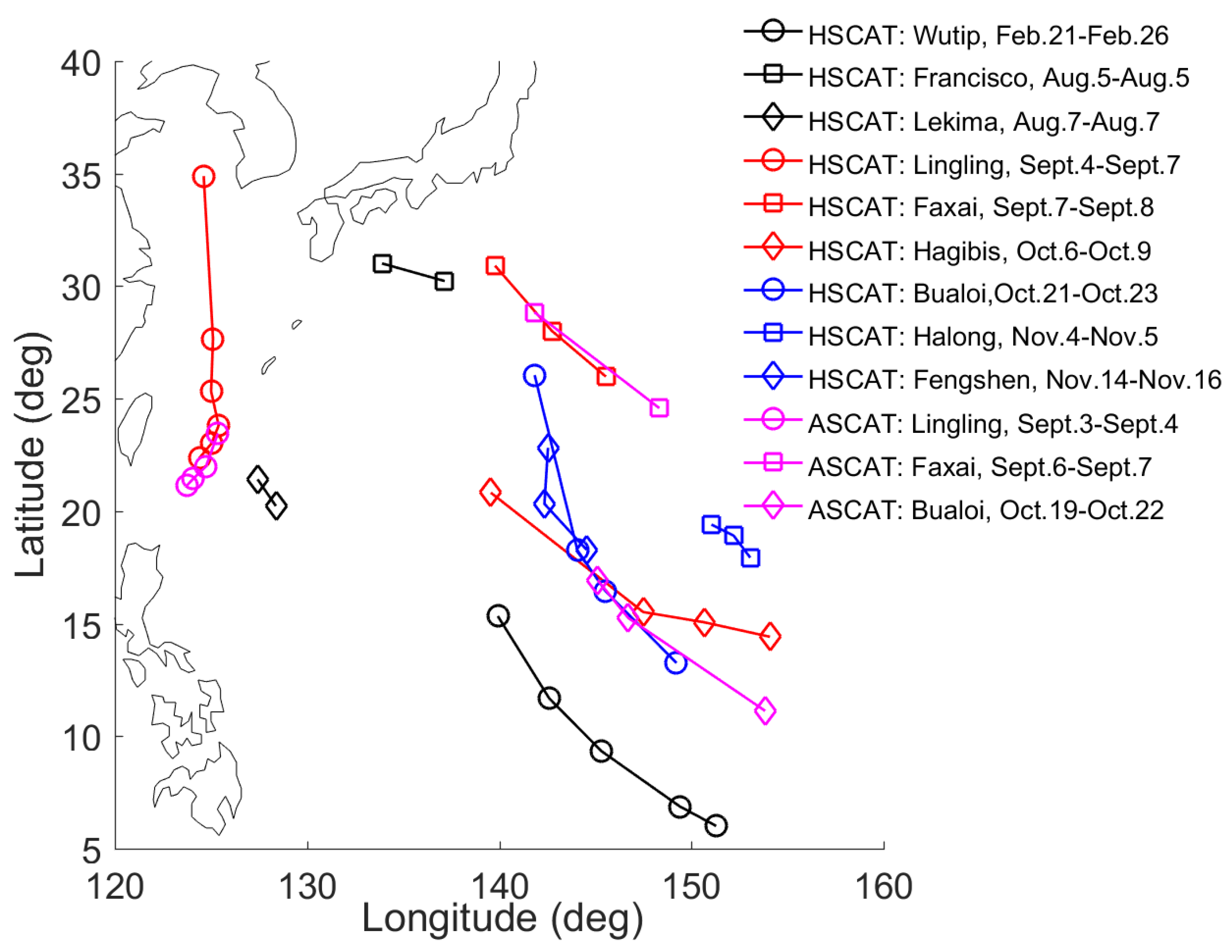
2. Data
3. Method
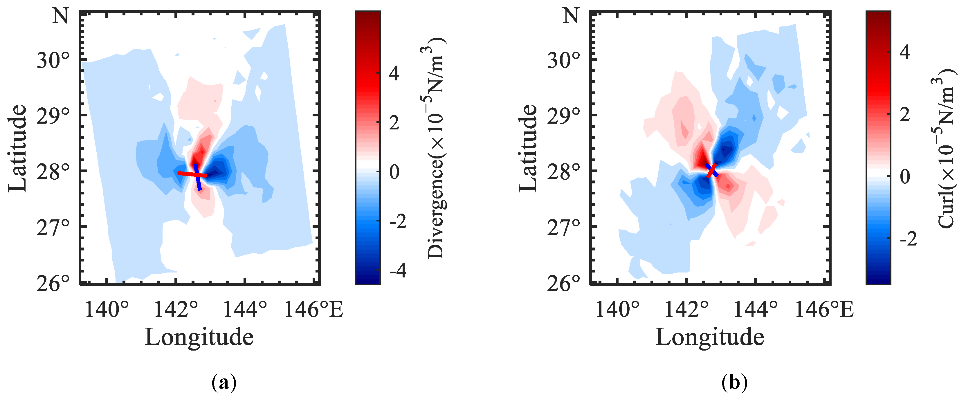
3.1. TC Center Location
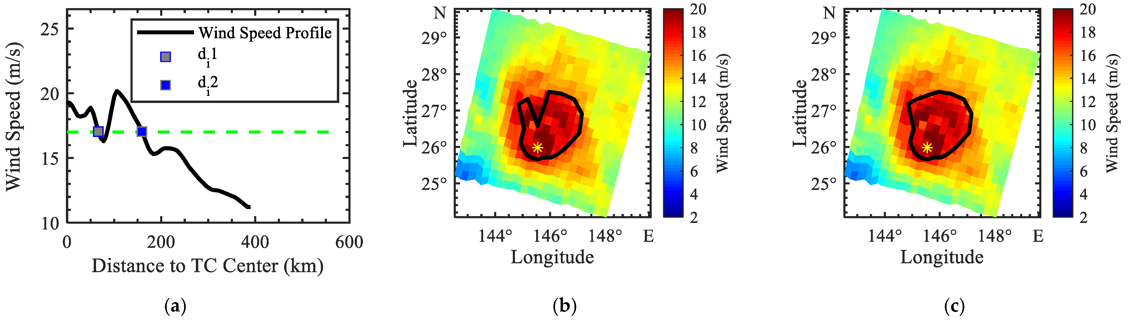
3.2. TC Wind Radii
4. Results
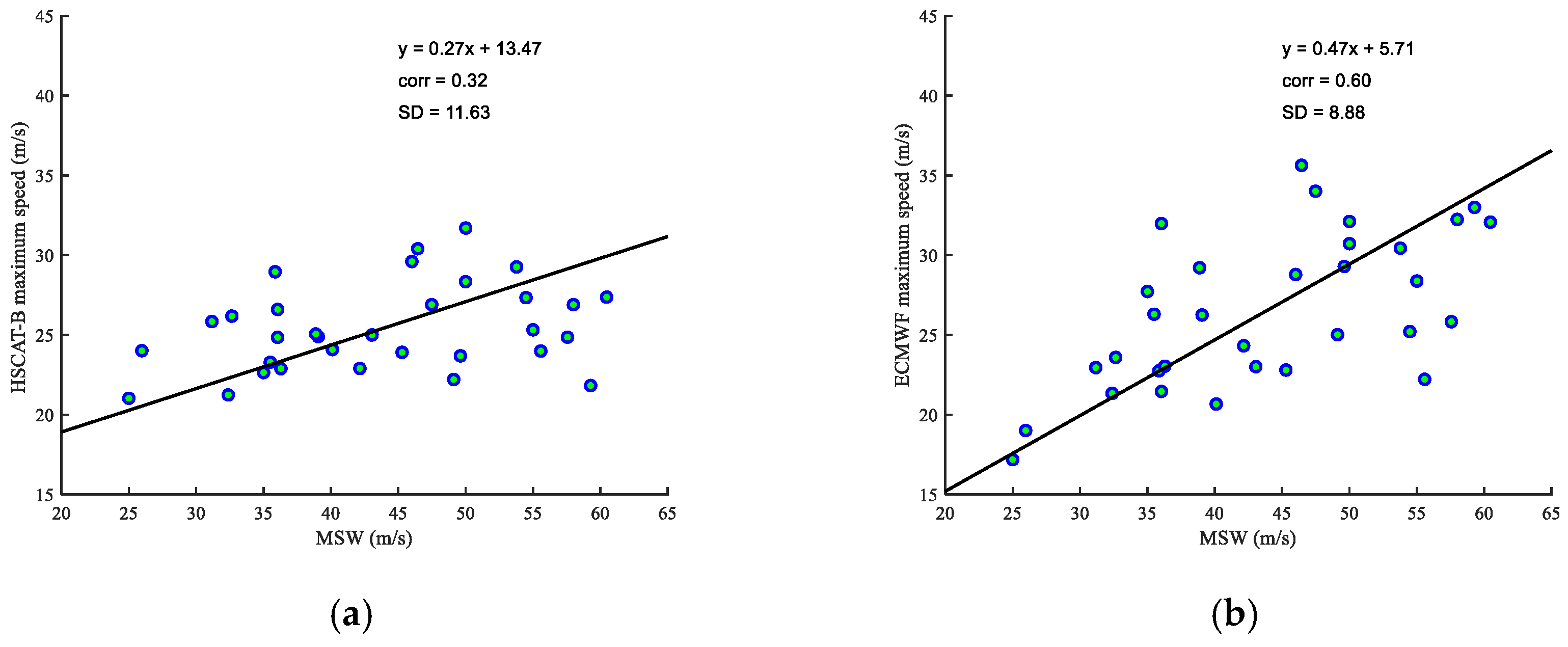
4.1. HSCAT Maximum Wind Speed versus Best-Track MSW
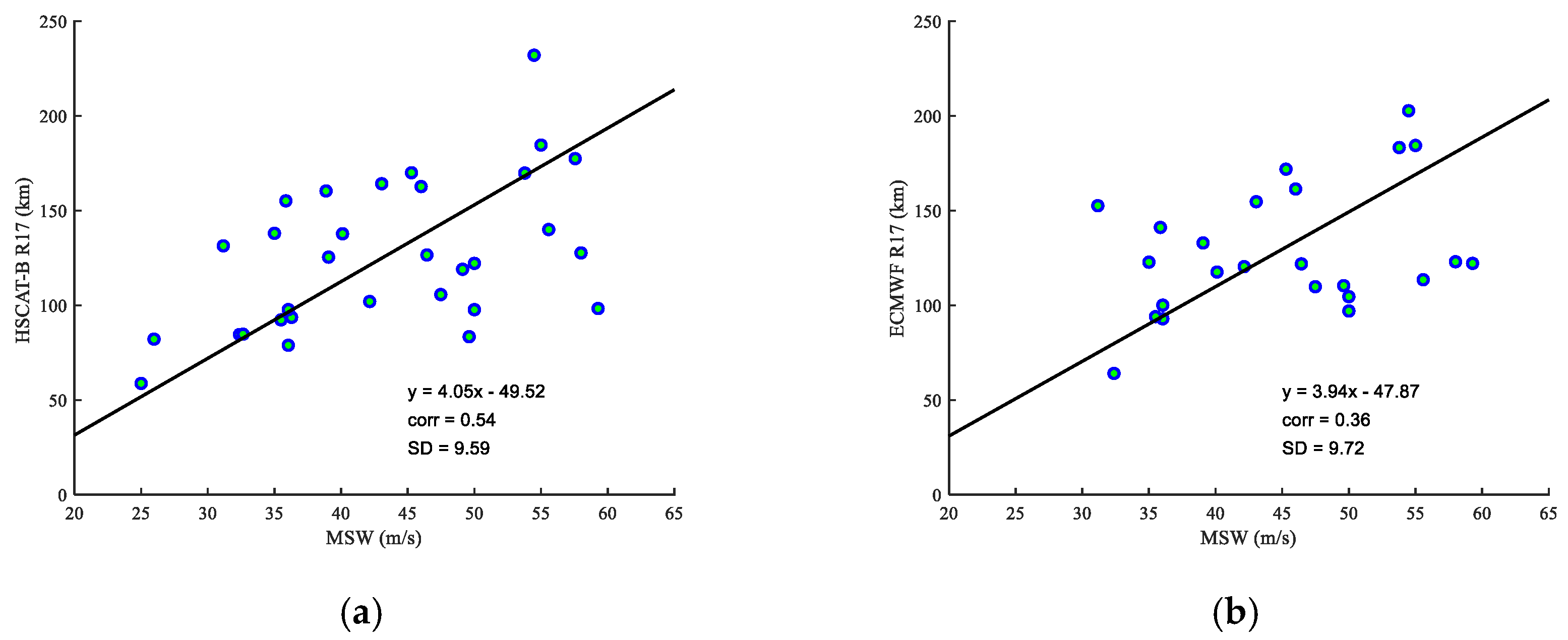
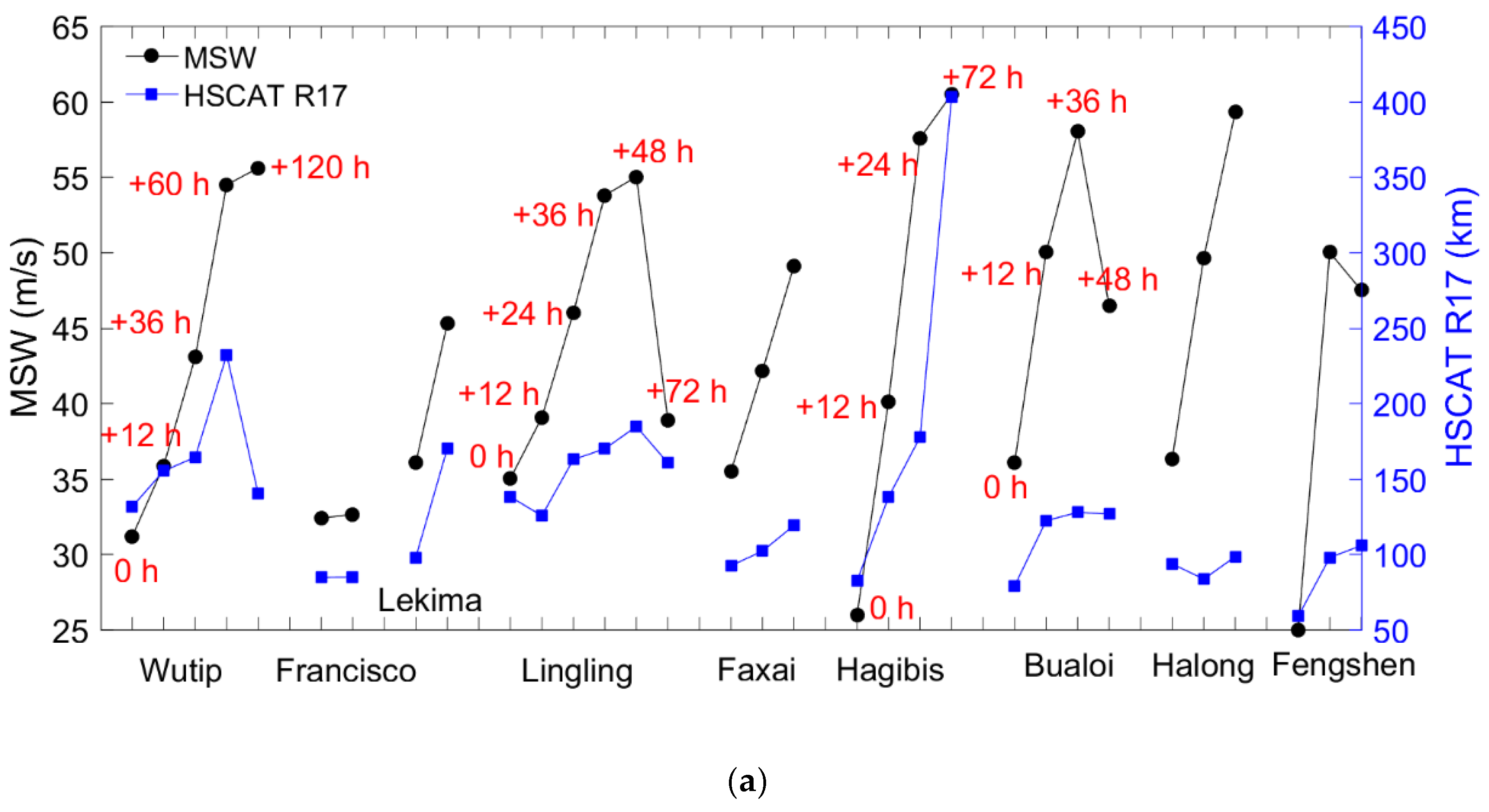
4.2. HSCAT Wind Radii versus Best-Track MSW
4.3. ASCAT Wind Radii versus Best-Track MSW
5. Discussion and Conclusions
Author Contributions
Funding
Institutional Review Board Statement
Informed Consent Statement
Data Availability Statement
Acknowledgments
Conflicts of Interest
References
- Hayes, S.P.; Mangum, L.J.; Picaut, J.; Sumi, A.; Takeuchi, K. TOGA-TAO: A Moored Array for Real-time Measurements in the Tropical Pacific Ocean. Bull. Am. Meteorol. Soc. 1991, 72, 339–347. [Google Scholar] [CrossRef] [Green Version]
- Sapp, J.; Alsweiss, S.; Jelenak, Z.; Chang, P.; Carswell, J. Stepped Frequency Microwave Radiometer Wind-Speed Retrieval Improvements. Remote Sens. 2019, 11, 214. [Google Scholar] [CrossRef] [Green Version]
- Morris, M.; Ruf, C.S. Determining Tropical Cyclone Surface Wind Speed Structure and Intensity with the CYGNSS Satellite Constellation. J. Appl. Meteorol. Clim. 2017, 56, 1847–1865. [Google Scholar] [CrossRef]
- Reul, N.; Tenerelli, J.; Chapron, B.; Vandemark, D.; Quilfen, Y.; Kerr, Y. SMOS satellite L-band radiometer: A new capability for ocean surface remote sensing in hurricanes. J. Geophys. Res. 2012, 117, C02006. [Google Scholar] [CrossRef] [Green Version]
- Meissner, T.; Ricciardulli, L.; Wentz, F.J. Capability of the SMAP Mission to Measure Ocean Surface Winds in Storms. Bull. Am. Meteorol. Soc. 2017, 98, 1660–1677. [Google Scholar] [CrossRef]
- Polverari, F.; Portabella, M.; Lin, W.; Sapp, J.W.; Stoffelen, A.; Jelenak, Z.; Chang, P.S. On High and Extreme Wind Calibration Using ASCAT. IEEE Trans. Geosci. Electron. 2021, 60, 1–10. [Google Scholar] [CrossRef]
- Ricciardulli, L.; Mears, C.; Manaster, A.; Meissner, T. Assessment of CYGNSS Wind Speed Retrievals in Tropical Cyclones. Remote Sens. 2021, 13, 5110. [Google Scholar] [CrossRef]
- Zhang, L.; Yin, X.; Shi, H.; Wang, Z.; Xu, Q. Estimation of wind speeds inside Super Typhoon Nepartak from AMSR2 low-frequency brightness temperatures. Front. Earth Sci. 2019, 13, 124–131. [Google Scholar] [CrossRef]
- Manaster, A.; Ricciardulli, L.; Meissner, T. Tropical Cyclone Winds from WindSat, AMSR2, and SMAP: Comparison with the HWRF Model. Remote Sens. 2021, 13, 2347. [Google Scholar] [CrossRef]
- Lecomte, P.; Crapolicchio, R.; Saavedra de Miguel, L. Cyclone Tracking with ERS-2 Scatterometer: Algorithm Performances and Post-processed Data Examples. In Proceedings of the ERS-ENVISAT Symposium Gothenburg (S), Gothenburg, Sweden, 16–20 October 2000. [Google Scholar]
- Brennan, M.J.; Hennon, C.C.; Knabb, R.D. The Operational Use of QuikSCAT Ocean Surface Vector Winds at the National Hurricane Center. Wea. Forecasting. 2009, 24, 621–645. [Google Scholar] [CrossRef] [Green Version]
- Seubson, S.; Suntana, O. Characterization of the Tropical Cyclones Wind Radii in the North Western Pacific Basin Using the ASCAT Winds Data Products. In Proceedings of the 2018 Progress in Electromagnetics Research Symposium (PIERS-Toyama), Toyama, Japan, 1–4 August 2018; pp. 1428–1433. [Google Scholar]
- Hu, T.; Wu, Y.; Zheng, G.; Zhang, D.; Zhang, Y.; Li, Y. Tropical Cyclone Center Automatic Determination Model Based on HY-2 and QuikSCAT Wind Vector Products. IEEE Trans. Geosci. Remote Sens. 2019, 57, 709–721. [Google Scholar] [CrossRef]
- Spencer, M.W. A Methodology for the Design of Spaceborne Pencil-Beam Scatterometer Systems. Ph.D. Thesis, Brigham Young University, Provo, UT, USA, 2001. [Google Scholar]
- Pramanik, S.; Sil, S. Assessment of SCATSat-1 Scatterometer Winds on the Upper Ocean Simulations in the North Indian Ocean. J. Geophys. Res. Oceans. 2021, 126, 6. [Google Scholar] [CrossRef]
- Bhowmick, S.A.; Kumar, R.; Kiran Kumar, A.S. Cross Calibration of the OceanSAT -2 Scatterometer With QuikSCAT Scatterometer Using Natural Terrestrial Targets. IEEE Trans. Geosci. Remote Sens. 2014, 52, 3393–3398. [Google Scholar] [CrossRef]
- Wang, Z.; Zhao, C.; Zou, J.; Xie, X.; Zhang, Y.; Lin, M. An improved wind retrieval algorithm for the HY-2A scatterometer. Chin. J. Oceanol. Limnol. 2015, 33, 1201–1209. [Google Scholar] [CrossRef]
- Figa-saldaña, J.; Wilson, J.; Attema, E.; Gelsthorpe, R.; Drinkwater, M.; Stoffelen, A.D. The Advanced Scatterometer (ASCAT) on the Meteorological Operational (MetOp) platform: A follow on for European wind scatterometers. Can. J. Remote Sens. 2002, 28, 404–412. [Google Scholar] [CrossRef]
- Stiles, B.W.; Yueh, S.H. Impact of rain on spaceborne ku-band wind scatterometer data. IEEE Trans. Geosci. Remote Sens. 2002, 40, 1973–1983. [Google Scholar] [CrossRef]
- Lin, W.; Portabella, M. Toward an Improved Wind Quality Control for RapidScat. IEEE Trans. Geosci. Remote Sens. 2017, 55, 3922–3930. [Google Scholar] [CrossRef] [Green Version]
- Liu, J.; Lin, W.; Dong, X.; Lang, S.; Yun, R.; Zhu, D.; Zhang, K.; Sun, C.; Mu, B.; Ma, J.; et al. First Results From the Rotating Fan Beam Scatterometer Onboard CFOSAT. IEEE Trans. Geosci. Remote Sens. 2020, 58, 8793–8806. [Google Scholar] [CrossRef]
- Wang, Z.; Zou, J.; Stoffelen, A.; Lin, W.; Verhoef, A.; Li, X.; He, Y.; Zhang, Y.; Lin, M. Scatterometer Sea Surface Wind Product Validation for HY-2C. IEEE J-STARS 2021, 14, 6156–6164. [Google Scholar] [CrossRef]
- Chan, K.T.F.; Chan, J.C.L. Size and Strength of Tropical Cyclones as Inferred from QuikSCAT Data. Mon. Weather Rev. 2012, 140, 811–824. [Google Scholar] [CrossRef]
- Guo, X.; Tan, Z. Tropical cyclone fullness: A new concept for interpreting storm intensity. Geophys. Res. Lett. 2017, 44, 4324–4331. [Google Scholar] [CrossRef]
- Wang, Z.; Stoffelen, A.; Zou, J.; Lin, W.; Verhoef, A.; Zhang, Y.; He, Y.; Lin, M. Validation of New Sea Surface Wind Products From Scatterometers Onboard the HY-2B and MetOp-C Satellites. IEEE Trans. Geosci. Remote Sens. 2020, 58, 4387–4394. [Google Scholar] [CrossRef]
- Ying, M.; Zhang, W.; Yu, H.; Lu, X.; Feng, J.; Fan, Y.; Zhu, Y.; Chen, D. An overview of the China Meteorological Administration tropical cyclone database. J. Atmos. Oceanic Technol. 2014, 31, 287–301. [Google Scholar] [CrossRef] [Green Version]
- Lu, X.; Yu, H.; Ying, M.; Zhao, B.; Zhang, S.; Lin, L.; Bai, L.; Wan, R. Western North Pacific Tropical Cyclone Database Created by the China Meteorological Administration. Adv. Atmos. Sci. 2021, 38, 690–699. [Google Scholar] [CrossRef]
- Merrill, R.T. A Comparison of Large and Small Tropical Cyclones. Mon. Weather Rev. 1984, 112, 1408–1418. [Google Scholar] [CrossRef] [Green Version]
- Liu, S.; Lin, W.; Wang, Z.; Lang, S. Determination of Tropical Cyclone Location and Intensity using HY-2B Scatterometer Data. Acta Oceanol. Sin. (Chin. Ed.) 2021, 43, 1–12. [Google Scholar]
- Shea, D.J.; Gray, W.M. The Hurricane’s Inner Core Region. I. Symmetric and Asymmetric Structure. J. Atmos. Sci. 1973, 30, 1544–1564. [Google Scholar] [CrossRef] [Green Version]
- Kimball, S.K.; Mulekar, M.S. A 15-Year Climatology of North Atlantic Tropical Cyclones. Part I: Size Parameters. J. Clim. 2004, 17, 3555–3575. [Google Scholar] [CrossRef]
- Lin, W.; Portabella, M.; Stoffelen, A.; Vogelzang, J.; Verhoef, A. On mesoscale analysis and ASCAT ambiguity removal. Q. J. R. Meteorol. Soc. 2016, 142, 1745–1756. [Google Scholar] [CrossRef] [Green Version]
- Xu, X.; Stoffelen, A. Improved Rain Screening for Ku-Band Wind Scatterometry. IEEE Trans. Geosci. Remote Sens. 2020, 58, 2494–2503. [Google Scholar] [CrossRef]


| TC Name | Correlation Coefficient | |||||
|---|---|---|---|---|---|---|
| R17 vs. MSW | HSCAT Wmax vs. MSW | ECMWF Wmax vs. MSW | R17 vs. MSLP | HSCAT Wmax vs. MSLP | ECMWF Wmax vs. MSLP | |
| Wutip | 0.53 | −0.36 | 0.33 | −0.54 | 0.36 | −0.34 |
| Wutip (<72 h) | 0.97 | 0.04 | 0.89 | −0.97 | −0.02 | −0.88 |
| Lingling | 0.83 | 0.63 | 0.56 | −0.84 | −0.61 | −0.54 |
| Hagibis | 0.79 | 0.76 | 0.91 | −0.81 | −0.78 | −0.92 |
| Bualoi | 0.86 | 0.16 | −0.08 | −0.87 | −0.17 | 0.09 |
Publisher’s Note: MDPI stays neutral with regard to jurisdictional claims in published maps and institutional affiliations. |
© 2022 by the authors. Licensee MDPI, Basel, Switzerland. This article is an open access article distributed under the terms and conditions of the Creative Commons Attribution (CC BY) license (https://creativecommons.org/licenses/by/4.0/).
Share and Cite
Liu, S.; Lin, W.; Portabella, M.; Wang, Z. Characterization of Tropical Cyclone Intensity Using the HY-2B Scatterometer Wind Data. Remote Sens. 2022, 14, 1035. https://doi.org/10.3390/rs14041035
Liu S, Lin W, Portabella M, Wang Z. Characterization of Tropical Cyclone Intensity Using the HY-2B Scatterometer Wind Data. Remote Sensing. 2022; 14(4):1035. https://doi.org/10.3390/rs14041035
Chicago/Turabian StyleLiu, Siqi, Wenming Lin, Marcos Portabella, and Zhixiong Wang. 2022. "Characterization of Tropical Cyclone Intensity Using the HY-2B Scatterometer Wind Data" Remote Sensing 14, no. 4: 1035. https://doi.org/10.3390/rs14041035