Decadal Lake Volume Changes (2003–2020) and Driving Forces at a Global Scale

Abstract

Lakes play a key role in the global water cycle, providing essential water resources and ecosystem services for humans and wildlife. Quantifying long-term changes in lake volume at a global scale is therefore important to the sustainability of humanity and natural ecosystems. Yet, such an estimate is still unavailable because, unlike lake area, lake volume is three-dimensional, challenging to be estimated consistently across space and time. Here, taking advantage of recent advances in remote sensing technology, especially NASA’s ICESat-2 satellite laser altimeter launched in 2018, we generated monthly volume series from 2003 to 2020 for 9065 lakes worldwide with an area ≥ 10 km². We found that the total volume of the 9065 lakes increased by 597 km³ (90% confidence interval 239–2618 km³). Validation against in situ measurements showed a correlation coefficient of 0.98, an RMSE (i.e., root mean square error) of 0.57 km³ and a normalized RMSE of 2.6%. In addition, 6753 (74.5%) of the lakes showed an increasing trend in lake volume and were spatially clustered into nine hot spots, most of which are located in sparsely populated high latitudes and the Tibetan Plateau; 2323 (25.5%) of the lakes showed a decreasing trend in lake volume and were clustered into six hot spots—most located in the world’s arid/semi-arid regions where lakes are scarce, but population density is high. Our results uncovered, from a three-dimensional volumetric perspective, spatially uneven lake changes that aggravate the conflict between human demands and lake resources. The situation is likely to intensify given projected higher temperatures in glacier-covered regions and drier climates in arid/semi-arid areas. The 15 hot spots could serve as a blueprint for prioritizing future lake research and conservation efforts.

1. Introduction

Over 80% of Earth’s liquid surface freshwater is stored in lakes [1], providing a wide range of services to human societies and wildlife [2,3]. However, there is mounting evidence that lakes globally have been undergoing rapid changes in the past decades [3,4,5,6,7]. To ensure a sustainable future for lakes, the Global Climate Observing System recently recognized lake water level and area, two indicators of lake volume, as essential climate variables [8]. An increasing number of countries have included lake conservation into their national sustainable development goals [9].

Based on repeated measurements of water level and area, changes in lake volume can be calculated, qualifying directly the water budget of a lake [10]. Although several initiatives are being undertaken for worldwide lake monitoring [10,11,12,13], a long-term assessment of the changes in global lake volume is still unavailable. Despite the fact that changes in two-dimensional lake area have been qualified by the GSW (i.e., Global Surface Water) database derived from Landsat images [14], the water volume of a lake is three-dimensional, tightly linked to water level, thus challenging to be estimated consistently across space and time [10]. Several radar missions, such as Topex/Poseidon, ENVISAT, Jason, and CryoSat-2, provide lake water level measurements [15,16,17]. Nevertheless, existing radar-based research still focused on a small proportion of global lakes with uneven temporal coverage, due to data quality issues or the difficulty of coordinating different sensors [13].

ICESat (i.e., Ice Cloud and land Elevation Satellite) and ICESat-2 have the potential to bring a significant step forward. The GLAS (i.e., Geoscience Laser Altimeter System) instrument onboard ICESat provides laser altimetry data from 2003 to 2009 with a fine spatial resolution (~70 m) [18]. The seven-year data collected by GLAS has triggered many applications in hydrological studies [19,20,21,22]. The newly available ATLAS (i.e., Advanced Topographic Laser Altimeter System) instrument onboard ICESat-2 extends the altimetry data to 2018–2020 (when this research was initiated), which have been successfully used to qualify the seasonal variability of lake water level at the global scale [23] and lake volume variations at the regional scale [24,25]. Thus, water level changes based on ICESat/ICESat-2 data, combined with area changes, offers an opportunity to estimate global lake volume changes spanning nearly two decades, with potentially high accuracy.

However, one challenge that needs to be engaged is the data gap of lake water level between 2009 and 2018 during which ICESat and ICESat-2 missions were disconnected. Fortunately, lake area is continuously available since the 1980s [14], and three approaches have been developed to reconstruct water level series from area series. The first approach is to assume a constant morphology for all lakes (e.g., a conical shape), such that lake area change can be geometrically linked to lake water level change [26]. However, this approach is challenging for a global application, because lake morphology differs across regions [10]. The second approach estimates the topographic slope of a lake using high-resolution DEM and terrain indices, based on the assumption that the topography surrounding a lake is indicative of lake morphology [27,28,29]. Although this approach has been used to provide a snapshot of global lake volume [30], the estimated changes in lake volume can be erroneous because the expansion or shrinkage of a lake is not isotropic as implicitly assumed by this approach. The third approach relies on existing observations of lake area and lake water level to build a regression between the two, and to obtain a regression slope [21,24,25]. Hence, this approach is purely data-driven, and is the most intuitive. However, unreasonable regression slopes (e.g., a negative slope value, which implies that the water level decreases with increasing area) were frequently obtained for many lakes, due to either measurement errors or the limited number of months during which both lake area and water level observations were available. For quality control purposes, previous research excluded lakes with unreasonable slopes from analysis [21,24,25,31], which caused a drastic reduction in the number of lakes studied.

In this study we developed a new method, built upon the abovementioned third approach, to reconstruct water level series from area series and therefore fill the data gap of lake water level between 2009 and 2018. An advantage of the new method is its ability to predict lake water level from lake area even with few paired observations between lake area and water level, thus largely improving the number of lakes that can be studied. Using our new method, combined with ICESat/ICESat-2 data and refined estimates of the GSW lake area, we provide a long-term (i.e., 2003–2020) assessment of the changes in lake volume at the global scale for 9065 lakes with an area ≥ 10 km². We then validate the estimated water levels and volumes using the ESA CCI (i.e., European Space Agency Climate Change Initiative) database and in situ measurements [13]. Further, the spatial pattern and driving forces of lake volume change are explored and discussed. Our results will hopefully be relevant for hydrological studies and the sustainable management of lakes worldwide.

2. Materials and Methods

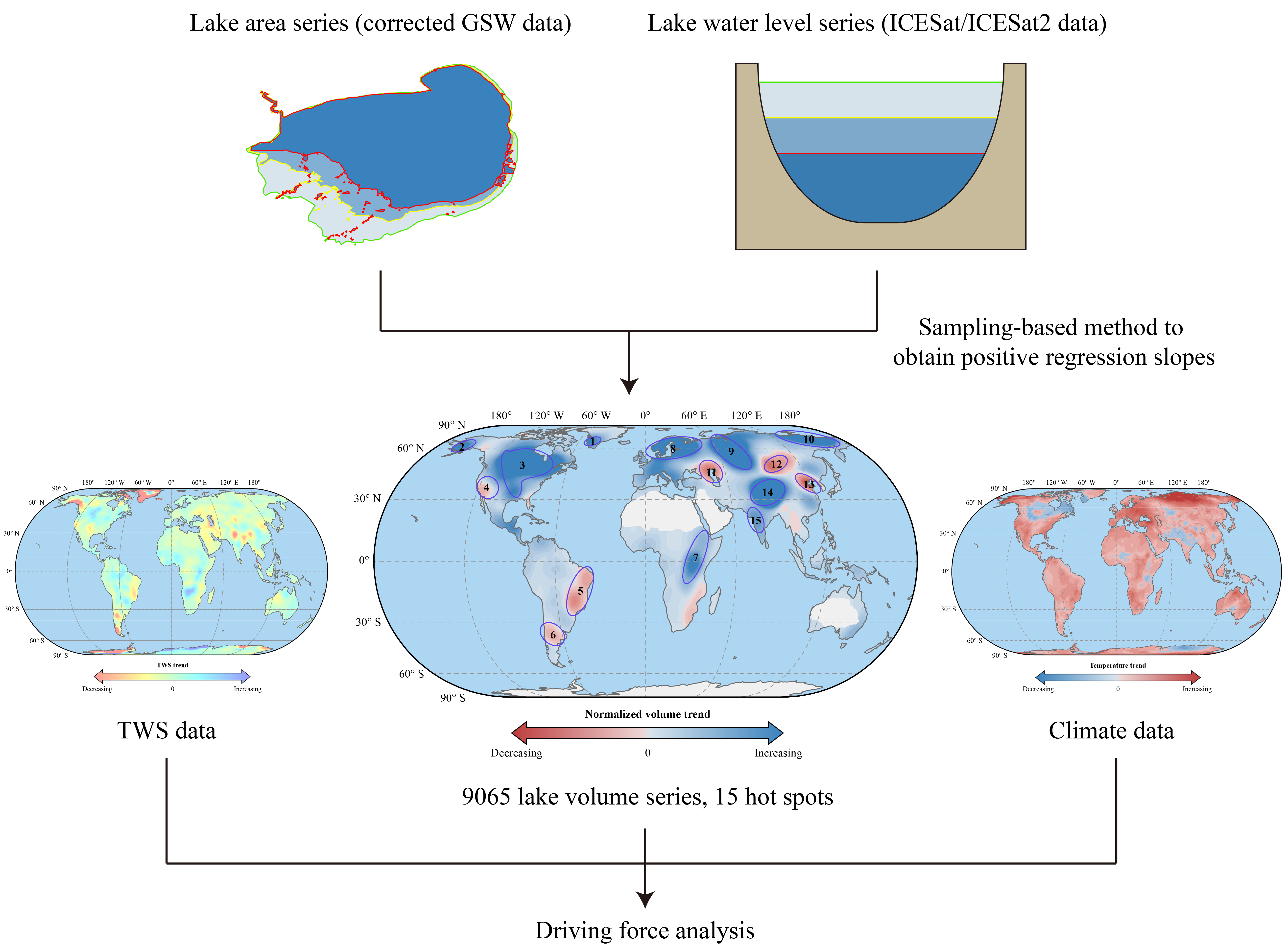
2.1. Methodological Framework

We located lakes with an area of at least 10 km² (16689 in total) using the HydroLAKES database [30], and then calculated a monthly time series of lake area for each lake using the GSW database, after controlling for quality issues such as cloud contamination (Figure S1). Note that months with no valid lake area observations were excluded from all subsequent analyses. We focused on lakes with an area larger than 10 km² because ICESat/ICESat-2 have relatively sparse observations over smaller lakes. To reconstruct a continuous series of lake water level, we calculated the regression slope (s) between lake water levels and lake area (i.e., $s=\frac{d level}{d area}$), using a new sampling-based method (Figure S2), and further generated area-derived water levels from 2003 to 2020. The monthly time series of lake area and water level were then combined to generate monthly lake volumes. The results were validated against in situ (Tables S1–S3) and satellite radar (i.e., ESA CCI database) measurements.

Lake volume changes were then compared to changes in terrestrial water storage (TWS) observed by the GRACE satellites (i.e., Gravity Recovery and Climate Experiment) [32,33]. Climate data were used to explore the driving forces of the observed lake volume changes. Spatial data processing was performed using the GDAL/OGR package [34] in Python. Lake volumes were calculated and analyzed using pracma and ggm packages in R [35,36,37]. The methodological framework is shown in Figure 1 and is explained in more detail below.

2.2. Locating Lakes

The locations and boundaries of 16689 lakes with an area of at least 10 km² were obtained from the HydroLAKES database (https://www.hydrosheds.org/page/hydro lakes; accessed on 18 January 2022). This database provides the state-of-art distribution of global inland water bodies by combing and correcting several near-global and regional datasets such as the SRTM water body data [30]. Reservoirs and natural lakes with regulation structures were included in this study and all are referred to as “lakes”.

2.3. Lake Area from the GSW Database

Pekel et al. generated a surface water database using Landsat images (https://global-surface-water.appspot.com/download; accessed on 18 January 2022) [14]. We used the occurrence map and monthly water history maps, two key components of the GSW database, to derive time series of lake area for lakes ≥10 km². Since the water history maps were affected by issues such as cloud contamination, data unavailability, and ETM+ sensor scan line failure [25], we rectified the water history maps using the method proposed by Zhao and Gao [38], which can be summarized as follows (Figure S1):

(1)

For each lake, a mask is generated by buffering its lake boundary as defined in the HydroLAKES database (Figure S1a). Extraction of lake area is confined within the masked region. A large buffer distance possibly includes surrounding water bodies, whereas a small one fails to capture the enlargement of the lake during the study period. The buffer distance (in meters) was chosen to be set as the ¼th power of lake area (in meters squared), after trial and error. This distance was validated to be neither too large (only 24 km for the Caspian Sea—the largest lake on Earth), nor too small (for 99% of the lakes, the maximum lake area did not exceed the buffer zone during 2003–2020).

(2)

The water history map of the GSW dataset describes whether each pixel was covered by water in a given month (Figure S1b), and the water occurrence map describes the frequency of each pixel marked as water bodies during the past decades (Figure S1c). We clipped the water occurrence map taking the cloud-contaminated water history map as a mask (Figure S1d), and then decided on an occurrence threshold (Figure S1e) [38], which was in turn used to binarize the water occurrence map and derive the final corrected lake area (Figure S1f). Note that we consider a lake to have a valid area observation in a month only if more than 10 pixels (~0.01 km²) are marked as water bodies in the corresponding water history map.

For each lake, we made certain that it had more than four valid area observations since 2003. To improve data quality, we removed outliers (if any) in each time series of lake area using a “hampel” filter [37], with the window length and the standard deviation of the filter set at 5 and 2, respectively, after trial and error.

2.4. Lake Water Level from ICESat and ICESat-2 Data

GLAH14, one of the level 2 ICESat/GLAS products, provides global surface elevation data from 2003 to 2009 (https://nsidc.org/; accessed on 18 January 2022). To compare the GLAH14 product with in situ measurements (height above mean sea level), we first extracted the high-quality elevation data, which were from the laser beams without signal saturation nor cloud contamination, and then converted them into orthometric heights using Equation (1) [39,40]:

$$h_{ortho}=h_{measure}-\mathrm{\Delta }{h}_{geoid}-\mathrm{\Delta }{h}_{ellipsoid}$$

(1)

where $h_{ortho}$ is the orthometric height above the EGM2008 geoid; $h_{measure}$ is the elevation with respect to the Topex/Poseidon ellipsoid (marked as “d_elev” in the released HDF5 files); $\mathrm{\Delta }{h}_{geoid}$ is the offset from the WGS84 ellipsoid to the EGM2008 geoid (“d_gdHt”); and $\mathrm{\Delta }{h}_{ellipsoid}$ is the offset from the Topex/Poseidon ellipsoid to the WGS84 ellipsoid (“d_deltaEllip”).

ATLAS on board ICESat-2 was launched in September 2018. Compared with GLAS, it has a smaller footprint (~17 m) and a finer spatial sampling interval (0.7 m along the track and 90 m across the track) [41], and thus observes many more lakes than ICESat (Figure S3). We used the ATL13, one of the level 3A ICESat-2/ATLAS products, to derive lake water levels from 2018 to 2020 [42]. As with the GLAH14 processing, we removed low-quality data, which came from strong beams or were contaminated by clouds, and then converted ellipsoid heights to orthometric heights. An additional parameter, known as significant wave elevation (h_wave), was used to further correct ICESat-2 measurements (Equation (2)) [24]:

$$h_{ortho}=h_{measure}-\mathrm{\Delta }{h}_{geoid}-h_{wave}$$

(2)

where $h_{measure}$ is the elevation with respect to the WGS84 ellipsoid (“ht_water_surf”) and the other symbols have the same meanings as in Equation (1).

We averaged ICESat/ICESat-2 $h_{ortho}$ from laser shots that fell in the central region of each lake (pixels with a 100% occurrence frequency in the GSW water occurrence map). This avoids the influence of ground laser shots on water level retrieval [22]. Note that if there exist multiple observations ($h_{ortho}$) for a lake within a month, we averaged these values to make the temporal resolution of water level data the same as that of area data. Outliers (if any) in each monthly mean water level time series were removed, using the “hampel” filter as mentioned above.

2.5. Area-Derived Water Level

As mentioned in the Introduction, we developed a new method to fill the data gap of water level. This method predicts lake water level from lake area using the ordinary least squares regression technique (Equations (3) and (4)):

$$h_t=s{A}_t+c+{\epsilon }_t$$

(3)

$$\widehat{h_t}=\widehat{s}{A}_t+\widehat{c}$$

(4)

where $h_t$ and $A_t$ are the water level and area at time $t$; ${\epsilon }_t$ is the error term; $s$ and $c$ are the regression slope and intercept, respectively; $\widehat{s}$ and $\widehat{c}$ are the estimated parameters, which are derived from Equation (3) using the ordinary least squares regression; and $\widehat{h_t}$ is the area-derived water level at time $t$.

More specifically, the method followed the idea of Monte Carlo simulation [43] and can be divided into the following steps (Figure S2):

(1)

We first counted the number of paired observations between lake area and lake water level (or, number of months in which both lake area and water level were observed). If the value is greater than or equal to four, proceed to step (2); otherwise, proceed to step (3). The threshold of four was decided after trial and error, and other values produced lower accuracy for the estimated water levels according to the validation against in situ data.

(2)

We sampled randomly two paired observations without replacement and calculated a regression slope between the sampled lake area and lake water levels. This step was repeated 2000 times and all positive slopes were kept.

(3)

We sampled randomly two water levels without replacement and recorded their months and years. Two lake area observations were then sampled from the same months of water levels but not necessarily from the same years. A regression slope was then calculated between the sampled lake area and lake water levels. This step was repeated 2000 times and all positive slopes were kept.

(4)

The final regression slope ($s$) was calculated as the median of all positive slopes. The 90% confidence interval ($s_5$ and $s_{95}$) of the slope was also calculated to quantify the uncertainty of our approach.

The threshold for the number of paired observations (i.e., at least four pairs) and the sampling times (i.e., 2000 times) were obtained by a trial-and-error process. The difference between in situ and area-derived water levels were the minimum when the two parameters were set to four and 2000, respectively (Figure S4).

Our method enabled us to estimate the regression slopes (s) for 9065 out of the 16,689 (54.3%) lakes ≥10 km² in area, in contrast to 948 lakes if this method was not applied. The sum of volumes of the 9065 lakes accounts for 98% of the total lake volume of the 16,689 lakes, according to the global lake volume estimations by Messager et al. [30].

Based on the estimated the regression slopes, we further reconstructed a continuous water level series from 2003 to 2020 as follows (Equation (5)):

$$h_t-h_{t_0}=s\left(A_t-A_{t_0}\right)$$

(5)

where $A$ and $h$ are the lake area and water level derived from lake area, respectively; $t$ is the month in which there was a valid area observation; $t_0$ is the first month between 2003 and 2020 in which there was a valid area observation; and $s$ is the regression slope calculated by our sampling-based method. The lower and upper limits of $h_t$ (i.e., $h_{t5}$ and $h_{t95}$) were also calculated by substituting s with $s_5$ and $s_{95}$, respectively.

2.6. Lake Volume Changes and Drivers

We then calculated a time series of lake volume ($V_t$) for each of the 9065 lakes [10,44,45]:

$$V_t=h_t\left(A_t+A_{t_0}+\sqrt{A_t{A}_{t_0}}\right)/3$$

(6)

where all symbols have the same meanings as in Equation (5). The lower and upper limits of $V_t$ were also calculated by substituting $h_t$ with $h_{t5}$ and $h_{t95}$, respectively.

After obtaining lake volume series, we calculated lake volume changes between 2003 and 2020 (i.e., $V_{2020}$ minus $V_{2003}$). To mitigate the impact of intra-annual variation in lake volume, V₂₀₂₀ and V₂₀₀₃ were represented by lake volumes in the same months of 2020 and 2003, respectively. Less than 2% (162/9065) of lakes had no volume in the same months of 2020 and 2003, so their $V_{2020}$ and $V_{2003}$ were represented by lake volumes in the same months of two closest neighboring years of 2020 and 2003, respectively (such as 2019 and 2004, depending on data availability).

Temporal trends in lake volume from 2003 to 2020 were also calculated, using the seasonal Kendall method [43]. This method separates the inter-annual trend of lake volumes from the intra-annual variation. Specifically, volumes were first grouped by month (Equation (7)), and then the inter-annual trend and its corresponding p value were calculated, as depicted in Equations (8)–(11):

$$\begin{array}{c}V=\left(V_1,V_2,\dots ,V_{12}\right)\\ V_i=\left(v_{i1},v_{i2},\dots ,v_{i{n}_i}\right)\end{array}$$

(7)

$$Tren{d}_{ijk}=\frac{v_{ij}-v_{ik}}{j-k},i=1,2,\dots ,12;j=k+1,k+2,\dots ,n_i;k=1,2,\dots ,n_i-1$$

(8)

$$S={{\displaystyle \sum }}_{i=1}^{12}{{\displaystyle \sum }}_{j=k+1}^{n_i}{{\displaystyle \sum }}_{k=1}^{n_i-1}sgn\left(v_{ij}-v_{ik}\right)$$

(9)

$$Var\left(S\right)={{\displaystyle \sum }}_{i=1}^{12}\frac{n_i\left(n_i-1\right)\left(2n_i+5\right)}{18}$$

(10)

$$Z=\{\begin{array}{c}\frac{S-1}{\sqrt{Var\left(S\right)}}, S>0\\ 0, S=0\\ \frac{S+1}{\sqrt{Var\left(S\right)}}, S<0\end{array}$$

(11)

where $V$ is a group of volume estimations, made up of subsamples $V_1$ through $V_{12}$ (one for each month); $V_i$ contains $n_i$ annual values from month $i$ (i.e., $v_{i1},v_{i2},\dots ,v_{i{n}_i}$); $Tren{d}_{ijk}$ is the possible trend value, which was calculated by any two estimated volumes in the same subsample. The inter-annual trend is the median of possible trend values; $sgn(\ast )$ is the sign function; and $Z$ is the standard normal variate. That is, we consider lake volume changes to be significant (p < 0.05) if $\left|Z\right|>1.96$.

To clearly present the spatial pattern of the trends in volume, we identified hot spots of lake change using the kernel density method. To do this, we first normalized the volumes of each lake using Equation (12):

$$V_t^{’}=(V_t-V_0)/\left(V_{max}-V_{min}\right)$$

(12)

where $V_t$ is the normalized volume at time $t$; $V_t$ is the volume value derived from Equation (6); $V_0, V_{max},$ and $V_{min}$ are the first, maximum, and minimum volume values, respectively, in the time series of lake volume. Normalization is necessary because the volumes differed in magnitude among lakes.

We then calculated the trends in the normalized volume for all lakes, and smooth the trends spatially using the kernel density method [46,47]:

$$Tren{d}_{\left(x,y\right)}=\frac{3}{\pi }{{\displaystyle \sum }}_{i=1}^{n}Tren{d}_i{(1-{(\frac{dis{t}_i}{radius})}^2)}^2$$

(13)

where ${Tren}_i$ is the trend of normalized volume series for lake $i$, calculated using the seasonal Kendall method; $Tren{d}_{\left(x,y\right)}$ is the smoothed trend at the location $\left(x,y\right)$; $dis{t}_i$ is the distance between lake $i$ and the location $\left(x,y\right)$; and $radius$ is the search radius.

Finally, to explore the possible driver of lake change, we calculated the Pearson’s r between time series of lake volume and of the ERA5 (i.e., ECMWF Reanalysis v5) monthly temperature, potential evapotranspiration, and precipitation [48].

2.7. Lake Volume Change versus TWS Change

TWS observed by the GRACE satellite reflects the amount of water stored on the Earth’s surface, including different forms of water such as lakes, groundwater, snow and ice, and glaciers [49]. To check whether directions of lake volume change are consistent with directions of TWS change, we compared the spatial pattern of lake volume change with that of TWS change [32,33,50]. Specifically, we obtained Tellus monthly mass grids from 2003 to 2017 using GEE (i.e., Google Earth Engine). We then extracted TWS series for each lake and calculated Pearson’s r between TWS and volume series.

3. Results

3.1. Accuracy Assessment of Lake Water Levels and Lake Volumes

The accuracy of ICESat/ICESat-2 data was assessed against the in situ water levels of 132 lakes (see Table S1 and Figure S5 for detailed information on these lakes). After eliminating systematic errors caused by the difference in reference ellipsoid by normalizing in situ and satellite-derived water levels, we obtained a Pearson’s r of 0.997 and a root mean square error (RMSE) of 0.375 m (Figure S6a). ICESat-2 showed a higher accuracy than ICESat (Figure S6a). Among the 132 lakes, 85% had a Pearson correlation coefficient (r) greater than 0.8, and 78% has a normalized RMSE (NRMSE, not influenced by the very different volumes of 132 lakes) lower than 30% (Table S1). We also compared water levels retrieved from ICESat/ICESat-2 with ESA CCI water levels. We found lower accuracy for ESA CCI product, as compared to the performance of ICESat/ICESat-2 (Figures S6a,b): the NRMSE of ICESat/ICESat-2 water levels was much lower than that of ESA CCI (0.5% vs. 22%). We therefore conclude that water levels retrieved from ICESat/ICESat-2 data are highly accurate.

Regarding the accuracy of area-derived water levels, although the RMSE was higher compared with the accuracy of water levels directly observed by ICESat/ICESat-2, the NRMSE remained low (Figure S6c): among the 132 lakes with in situ water levels, 94 showed NRMSEs lower than 30% (Table S2). This indicates that our proposed sampling-based approach is effective.

The uncertainties of estimated lake volumes were also assessed. Compared with lake water levels, lake volumes are much more difficult to be measured on the ground. Ultimately, we collected in situ volume measurements for 14 lakes (see Table S3 and Figure S5 for detailed information on these lakes). A Pearson’s r of 0.976 and an RMSE of 0.568 km³ were obtained (Figure S7), and 12 lakes had an NRMSE lower than 30% (Table S3), suggesting that the estimated lake volumes are reliable.

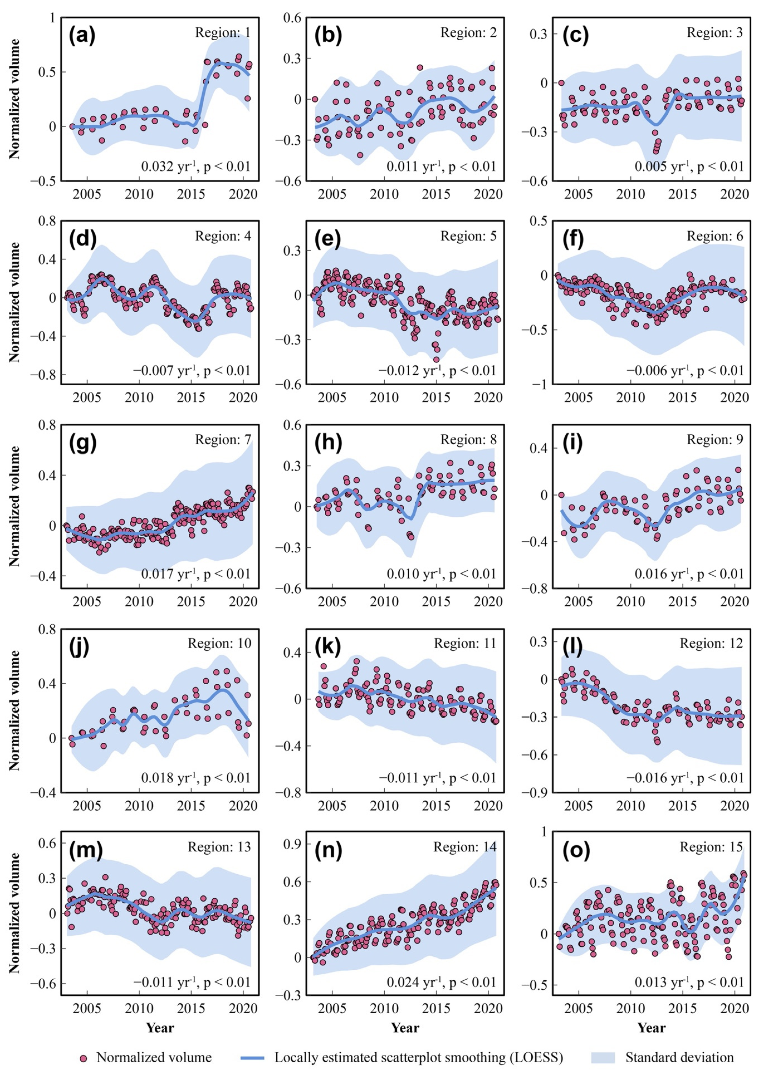
3.2. Lake Volume Changes from 2003 to 2020

From 2003 to 2020, the total volume of the 9065 lakes increased by 597 km³ (90% confidence interval 239–2618 km³). Increases in lake volume were observed in 6049 (66.7%) lakes. Regarding the temporal trends in lake volume (Figure 2a), 6753 (74.5%) of the lakes showed an increasing trend whereas 2312 (25.5%) showed a decreasing trend; 54.8% (4964/9065) of the lakes experienced significant volume changes (p < 0.05), with 44.6% increasing and 10.2% decreasing. We identified 15 hot spots of lake volume change (Figure 2b). Nine of the 15 hot spots were dominated by increasing trends in lake volume, including southern Greenland (region 1), western Alaska (region 2), central North America (region 3), central East Africa (region 7), northern Europe (region 8), western Russia (region 9), eastern Siberia (region 10), the Tibetan Plateau (region 14), and western India (region 15). Six hot spots were found to be dominated by decreasing trends in lake volume, including western United States (region 4), southeastern Latin America (region 5), southern Latin America (region 6), central Asia (around Caspian Sea, region 11), the western Mongolian Plateau (region 12), and northern China (region 13).

We explored the temporal changes in lake volume in these hot spots (Figure 3). Southern Greenland (region 1, Figure 3a) showed the largest increasing trend (0.032 per year, or a 3.2% annual increase), due to an acceleration in lake expansion occurring around 2015. The Tibetan Plateau (region 14, Figure 3n) showed the second largest increasing trend (0.024 per year), followed by eastern Siberia (region 10, Figure 3j, 0.018 per year), central East Africa (region 7, Figure 3g, 0.017 per year), and western Russia (region 9, Figure 3i, 0.016 per year). The largest decrease in lake volume was observed in the western Mongolian Plateau (region 12, Figure 3l, −0.016 per year, or a 1.6% annual decrease), followed by southeastern Latin America (region 5, Figure 3e, −0.012 per year), and northern China (region 13, Figure 3m, −0.011 per year). Other regions such as central Asia and western United States showed smaller decreasing rates (Figure 3d,f). We verified that the drastic lake volume changes occurred in some regions (such as regions 12 and 14) are not due to calculation errors by checking the lake shoreline changes of typical lakes (Figure S8).

3.3. Lake Volume Changes versus TWS Changes

We then explored whether the directions of lake volume change are consistent with the directions of the total water resource changes in a region. For this purpose, trends in lake volume were compared with trends in TWS observed by the GRACE satellite. The spatial pattern of lake trends was generally consistent with that of TWS trends: trends in lake volume of 6526 (72%) of the lakes correlated positively with trends in TWS (Figure 4), although some correlations were inevitably insignificant (Figure S9). Trends in lake volume correlated negatively with TWS trends in 28% of the lakes which, however, were mainly distributed in Northern Hemisphere and the southern Tibetan Plateau, pointing to glacier and permafrost-related lake inflation. However, some lakes in densely populated regions such as northern and eastern China (Figure 4) also showed opposite trends between TWS and lake volume, suggesting intense human impacts. These results generally support the view that lakes are “sentinels” of surface water and climate changes [51], except for in regions with strong human interventions on lakes.

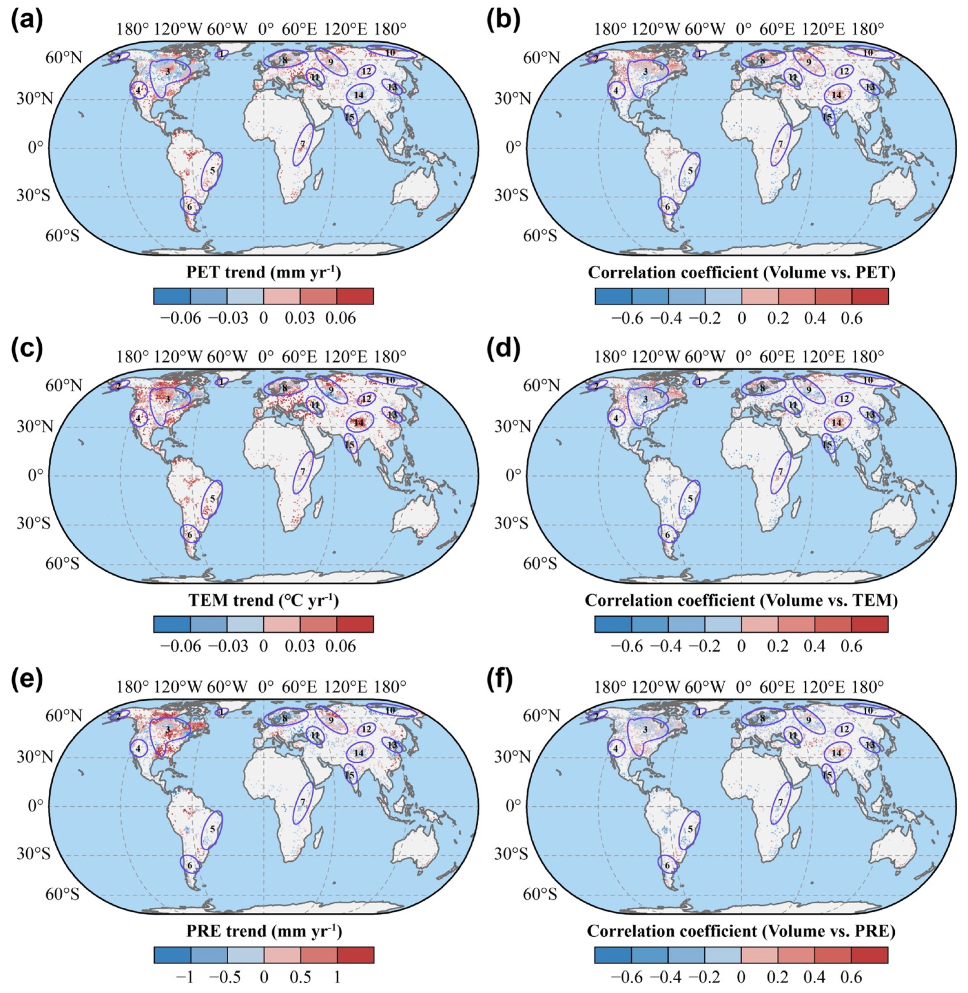
3.4. Climatic Drivers of Lake Volume Change

To further explore the climatic drivers of lake volume change, we calculated trends in three climatic factors (temperature, precipitation, and potential evapotranspiration), and performed correlation analyses between lake volume and each of the three climatic factors.

Seen from Figure 5, the impacts of climate change on lake volume were complex. We identified three types of climate-related lake changes: lake increase due to rising temperature, lake increase driven by wetter climate, and lake decrease caused by drier climate. A last category lumped all lake changes weakly associated with any of these three climate trends.

Lake volume increase due to rising temperature was mainly found in high-latitude and mountainous regions (regions 1, 2, 8, 10, and 14), suggesting indirectly the influences of glacier melt and permafrost thaw on lake volume changes. For instance, in southern Greenland (region 1), trends in lake volume correlated positively with rising temperature in 81% of the lakes (regional mean rate of 0.019 °C per year, Figure 5c,d). Similarly, in the Tibetan Plateau (region 14), 80% of the volume trends correlated positively with rising temperature, although 63% also correlated with increasing precipitation (Figure 5d,f).

Lake volume increase driven by wetter climate was mainly found in regions 3, 9, and 15. For instance, in western India (region 15), PET decreased with a regional average rate of −0.203 mm per year (Figure 5a); 98.6% of the increasing trends in lake volume in this region correlated negatively with the PET trends (Figure 5b). Region 3 (central North America) is large in area, extending ~30 degrees in latitude and ~60 degrees in longitude. This region experienced increased amount of precipitation in its southern and eastern parts, and decreased PET in its northern and western parts (Figure 5a,c). Consequently, 25.4% of the volume trends showed positive correlations with precipitation, and 52% showed negative correlations with PET (Figure 5b,f).

The third type of lake change (i.e., lake volume decrease caused by drying climate) was observed in regions 4, 5, 6, 11, 12, and 13, most of which are the world’s arid and semi-arid areas with high population densities. Region 4 (western United States) experienced increased PET and temperature during the study period (Figure 5a,c), although precipitation also slightly increased (Figure 5e). Except for this region, all the other five regions experienced strong drying climates characterized by rising temperature (regional averaged rate of 0.040, 0.024, 0.049, 0.041, and 0.039 °C, respectively), decreasing precipitation (regional averaged rate of −0.452, −0.271, −0.448, −0.134, −0.202 mm per year, respectively), and increasing PET (regional averaged rate of 0.198, 0.239, 0.256, 0.100, 0.170 mm per year, respectively) (Figure 5a,c,e). As a result, trends in lake volume of 80%, 53%, 67%, 60%, and 56% of the lakes in these five regions, respectively, correlated negatively with the rising temperature (Figure 5d).

Only in region 7 were lake changes weakly associated with climate. A drier climate was observed (increasing temperature, increasing PET, and decreasing precipitation) but lake volumes increased (Figure 5a,c,e).

4. Discussion

4.1. GSW and ICESat/ICESat-2 Data for Estimating Lake Volume Changes

Accurate and long-term information on lake volume is essential for water budget assessment and water resource management [1]. To monitor long-term changes in global lake volume, this study used the most recent advances in satellite remote sensing: the Landsat-based GSW database and the ICESat/ICESat-2 altimetry data.

The GSW database was produced using a massive number of Landsat images and various data mining techniques (e.g., expert system and visual analytics) [14]. This database provides accurate information about the dynamics of the Earth’s surface waters, which has been widely used in hydrological and ecological studies [52,53,54]. Here, we further refined the GSW layers to alleviate the impacts of clouds and scan line failure, using the method of Zhao and Gao [38] (Figure S1). The rectified lake area laid a solid foundation for subsequent estimation of lake volume changes.

Seminal research has demonstrated the large potential of remote sensing data for retrieving lake water levels, using mainly satellite radar data (e.g., Topex/Poseidon, ENVISAT, Jason, and CryoSat-2) [10,13,15,16,17]. Our results indicated that ICESat and ICESat-2 data had measurement errors of 35.5 cm and 26.0 cm, respectively (Figure S6a), better than previous radar measurements (Figure S6b) [55]. Moreover, compared with the ESA CCI database, a typical satellite radar-based water level product, ICESat/ICESat-2 observed more medium-sized lakes (i.e., lakes with an area of 10–50 km²), which are important habitats and water supplies in arid and semi-arid regions [5]. Another operating altimeter, GEDI (i.e., Global Ecosystems Dynamics Investigation) lidar onboard the ISS (i.e., International Space Station) has a theoretical observation capability comparable to GLAS or ATLAS due to its small footprint (~25 m). However, the orbital inclination angle of the ISS is 51.6°, which prevents the GEDI lidar from observing lakes at high latitudes [56]. Thus, ICESat/ICESat-2 altimetry data currently remains the best option for global-scale lake water level inversion. The upcoming Surface Water and Ocean Topography (SWOT) satellite mission will soon enable a more comprehensive estimate of lake volume, including the exceedingly small water bodies (<1 km² in area) [57] over which ICESat/ICESat-2 laser shots are sparse; thus, it is expected to contribute enormously to the conservation of global lakes.

4.2. Reconstructing Time Series of Lake Water Levels from Lake Area

Although lake area was continuously available throughout our study period (i.e., 2003–2020), lake water level was unavailable between 2009 and 2018. This problem challenged the trend analysis of lake volume. Three approaches have been developed for reconstructing time series of lake water levels from lake area, namely the morphology-based approach [26], the topography-based approach [27,28,29], and the data-driven approach [21,24,25] (see the Introduction section for details).

In this study, we used the third approach but extended it to tackle the challenge of unreasonable regression slope. Our proposed method, or the sampling-based method, gap-filled lake water levels for an unprecedented number of lakes (9065) with high accuracy. Comparing area-derived lake water levels against in situ measurements, we obtained a Pearson’s r of 0.901, an RMSE of 2.223 m, and an NRMSE of 3.2% (Figure S6c), which is comparable with existing case studies [25]. To test the accuracy of our approach more strictly, we used a worst-case scenario by applying our approach on Lake Hongze, one of the five largest freshwater lakes in China (Figure S10). Lake Hongze connects with several tributaries of the Yantgtze River, thus having an extremely irregular lake outline and a large seasonality in lake area. However, its seasonality in lake water level is much smaller under normal climate conditions. We found similar trends between area-derived and in situ time series of water level, with a Pearson’s r of 0.55 and an RMSE of 0.423 m (Figure S10), improving our confidence in the sampling-based approach.

We also compared our approach with the second approach that estimates the topographic slope of a lake. Using the topographic slopes provided by Messager et al. [30] and by assuming a circular lake boundary (see Figure S11 for details), we converted lake area changes into lake water level changes. However, we obtained less accurate results (NRMSE of 48.0% in Figure S11, compared to 3.2% in Figure S6c), suggesting that our sampling-based method is the best option currently available for interpolating lake water level from lake area.

It is worth noting that the accuracy of our method depends on the number of paired observations between lake area and lake water level. As shown in Figure S12, a significantly negative correlation was obtained between the accuracy of the estimated water levels and the number of paired observations (r = −0.195, p = 0.025). This is expected because paired observations were the inputs of our sampling-based method. With the accumulation of ICESat-2 data in the near future, our methods are expected to monitor the dynamics of a larger number of lakes, with possibly higher accuracy. With more ICESat-2 observations, it is also possible to quantify more accurately the codynamics between lake area and lake water level based on stratified sampling. We here established a constant, linear regression slope (between lake area and lake water level) per lake. However, the codynamics between lake area and lake water level could be nonlinear or time-dependent, which have been reported in, e.g., Lake Urmia, Lake Mead, and Lake Tana [20,31].

4.3. Validation and Uncertainties Assessment of the Estimated Lake Volumes

Prior to the analysis of lake volume changes, we assessed the accuracy of the estimated lake volumes. In spite of the difficulty of measuring lake volume on the ground, we were able to compile in situ lake volumes for 14 lakes from multiple sources (Table S3). To our knowledge, this dataset is the largest compilation for the validation of satellite-based lake volumes. Compared with in situ volumes, our estimated volumes showed NRMSEs ranging from 3.5% to 37.5%, which are similar to a previous estimation based on 30 years of altimetry data [31].

The validation also confirmed that two major results of this study are robust. First, our calculation that 9065 lakes increased in volume by 597 km³ with a 90% confidence interval of 239–2618 km³, is reliable. Seen from Table S3, 82.2% of the in situ volumes fell within the 90% confidence interval of the estimated volumes. Second, the trends in lake volume presented in Figure 2 are also reliable. For 11 out of 14 lakes with in situ volumes, correlation coefficients between estimated and in situ volumes were higher than 0.7 (Table S3). Further exploring the time series of lake volume for three typical lakes (Figure S13), we found highly similar trends between estimated and in situ volumes (r > 0.95), despite some shifts in the seasonal amplitude (Figure S13c). In addition, lake volume trends were highly consistent with TWS trends (Figure 4)—further evidence that the volume trends presented in Figure 2 are reliable.

4.4. Drivers of Lake Volume Change

Our results indicated large regional differences in the changes in lake volume attributed to several climatic drivers. The most prominent lake change is the temperature-driven increase in lake volume in high-latitude regions and in the Tibetan Plateau [58]. TWS decreased significantly in these regions [44] and correlated negatively with lake volume trends (Figure 4). However, this phenomenon is unsustainable as loss of glaciers will eventually deplete freshwater resources, thus threatening Earth’s long-term water supply.

The second-most prominent lake change is the worldwide lake decrease caused by drier climatic conditions (regions 4, 5, 6, 11, 12, and 13), especially in the arid and semi-arid areas (regions 5, 6, 11, 12, and 13). In western United States (region 4, located in the western of the Rocky Mountains), severe droughts and over-extraction of groundwater have caused a significant decrease in regional water resources [59]. Previous research found decreasing groundwater levels [60,61,62] and loss of forest canopy moisture in this region [63]. Our finding of decreasing lake volume is in line with these drying ecosystem conditions. Regions 5, 6, 11, 12, and 13 are the world’s major arid and semi-arid areas. The decreasing lake volume in these regions might directly impact local environment and social development, given the high dependence on freshwater in arid and semi-arid regions [50,64].

Compared with the above two types of lake changes, lake increase caused by wetter climatic conditions is much rarer. One such example is the central North America (region 3). This region suffered repeated droughts during 2001–2003, then received excessive precipitation in the following years, explaining the observed increasing lake volume. Another example is western India (region 15)—one of the world’s most densely populated regions. The widespread increase in lake volume in this region could be caused by a strengthening of the Indian Monsoon in the past decades [65].

In central East Africa (region 7), lake changes were found to be largely inconsistent with climate change. Interestingly, this region is known for anthropogenic practices involving dam construction, building of hydropower stations, and human management of lakes [66,67].

It should be noted that the same climatic drivers could have also been revealed by correlating lake area (instead of lake volumes) and climatic factors. This is because we gap-filled lake water levels using a linear regression between lake area and water levels, and then calculated lake volumes combining lake area and water levels. However, in reality, lake volume or water level changes could be inconsistent with lake area changes because of the complexity in three-dimensional lake topography [20,31]. With more water level observations in the future, it will be interesting to explore the nonlinear relationship between lake water level and area, and to expect different drivers of lake area and lake volume changes in some regions.

It should also be noted that our analysis only tried to uncover the dominant climatic driving forces of lake changes at the regional scale. At the local scale, human interventions also contributed largely to the observed lake changes. Previous studies reported lake changes caused by various forms of human activities, including but not limited to water diversion, irrigation [68], economic activities [6], and open-pit coal mining [5]. For instance, the world’s largest lake—the Caspian Sea in central Asia—is drying largely due to irrigation [68]. In the Mongolian Plateau, open-pit coal mining destroyed groundwater aquifers and reduced lake inflows [69]. In the North China Plain, lake refilling and inter-basin water transfer increased the water storages of some lakes, thus rescued the drying lakes. In northern and eastern China, agricultural irrigation, lake impoldering, and groundwater extraction have had severe impacts on many local lakes [70]. In the western United States, excessive groundwater pumping has led to a water crisis, and has therefore placed a heavier burden on lakes to supply water to human societies. Reconciling the increasing human demand with the ever-changing surface water resources remains a key challenge to sustainable development goals pledged by many countries.

5. Conclusions

Our study provided the first long-term (2003–2020) assessment of the changes in lake volume for 9065 lakes ≥10 km² on Earth. A new sampling-based method was developed to fill the data gap of water level between 2009 and 2018, and to reconstruct a continuous time series of lake water level from 2003 to 2020; 74.5% (6753 out of 9065) of the lakes showed increasing trends in volume whereas 25.5% showed decreasing trends. A net increase of 597 km³ (90% confidence interval 239–2618 km³) in the total lake volume was observed. Our results also indicated large regional differences in the changes in lake volume attributed to several climatic drivers. Against the backdrop of climate changes, human activities also contributed to the observed lake changes at the local scale in central East Africa, central Asia, and northern China.

Behind the net increase in total lake volume are spatially uneven lake changes, with increase in lake volume concentrated in the high latitudes and the Tibetan Plateau, and decrease in lake volume mainly found in arid/semi-arid areas. These results uncovered emerging issues in surface water sustainability. Firstly, in high latitudes and the Tibetan Plateau, lakes are abundant and population density is low (average population density per square kilometer is 36.5 person), but lake volumes increased mainly due to warming-induced glacier melt. This phenomenon is unsustainable as loss of glaciers will eventually deplete freshwater resources, thus threatening Earth’s long-term water supply. Portions of the glacial lakes even have the risk of sudden “outburst” floods, particularly in the geologically active Tibetan Plateau [71]. Secondly, a large population (~793.7 million—2.4 times the population of the United States in 2020) rely on lakes as main sources of freshwater in arid and semi-arid regions. Unfortunately, lake volumes further decreased in these regions, which has already impacted local environment and social development [5], and could even lead to the collapse of an entire regional economy, as in the case of the demise of the Aral Sea [72]. Moreover, since lake changes are indicative of surface water changes (Figure 4), lake volume decreases in arid/semi-arid regions also imply a looming water crisis involving not only lake shrinkages but also, e.g., dropping groundwater levels.

Seen from a global perspective, the observed spatially uneven lake volume changes exacerbate the tension, which are already high, between lake services and human demands. The situations are likely to worsen given projected higher temperature in glacier-covered regions and drier climate in arid/semi-arid regions, let alone the worldwide increasing human demands on surface water resources. It is for these reasons that continued monitoring and sustainable management of lakes are needed. In the near future, ICESat-2, GEDI, and the upcoming SWOT missions will jointly provide more observations of lake water level and lake volume over a larger number of lakes [57]. We will therefore constantly refine and update our estimations. The results of this study, especially the 15 hot spots, could serve as a blueprint for prioritizing lake research and conservation efforts, and are thus expected to contribute to a sustainable future for global lakes.

References

1. Woolway, R.I.; Kraemer, B.M.; Lenters, J.D.; Merchant, C.J.; O’Reilly, C.M.; Sharma, S. Global lake responses to climate change. Nat. Rev. Earth Environ. 2020, 1, 388–403. [Google Scholar] [CrossRef]
2. Dudgeon, D.; Arthington, A.H.; Gessner, M.O.; Kawabata, Z.I.; Knowler, D.J.; Lévêque, C.; Naiman, R.J.; Prieur-Richard, A.H.; Soto, D.; Stiassny, M.L.; et al. Freshwater biodiversity: Importance, threats, status and conservation challenges. Biol. Rev. 2006, 81, 163–182. [Google Scholar] [CrossRef] [PubMed]
3. Rinke, K.; Keller, P.S.; Kong, X.; Borchardt, D.; Weitere, M. Ecosystem Services from Inland Waters and Their Aquatic Ecosystems. In Atlas of Ecosystem Services: Drivers, Risks, and Societal Responses; Schröter, M., Bonn, A., Klotz, S., Seppelt, R., Baessler, C., Eds.; Springer: Berlin/Heidelberg, Germany, 2019; pp. 191–195. [Google Scholar]
4. Grafton, R.Q.; Pittock, J.; Davis, R.; Williams, J.; Fu, G.; Warburton, M.; Udall, B.; McKenzie, R.; Yu, X.; Che, N.; et al. Global insights into water resources, climate change and governance. Nat. Clim. Chang. 2013, 3, 315–321. [Google Scholar] [CrossRef]
5. Tao, S.; Fang, J.; Zhao, X.; Zhao, S.; Shen, H.; Hu, H.; Tang, Z.; Wang, Z.; Guo, Q. Rapid loss of lakes on the Mongolian Plateau. Proc. Natl. Acad. Sci. USA 2015, 112, 2281–2286. [Google Scholar] [CrossRef] [PubMed] [Green Version]
6. Wurtsbaugh, W.A.; Miller, C.; Null, S.E.; DeRose, R.J.; Wilcock, P.; Hahnenberger, M.; Howe, F.; Moore, J. Decline of the world’s saline lakes. Nat. Geosci. 2017, 10, 816–821. [Google Scholar] [CrossRef]
7. Pham-Duc, B.; Sylvestre, F.; Papa, F.; Frappart, F.; Bouchez, C.; Crétaux, J.F. The Lake Chad hydrology under current climate change. Sci. Rep. 2020, 10, 5498. [Google Scholar] [CrossRef] [PubMed] [Green Version]
8. Bojinski, S.; Verstraete, M.; Peterson, T.C.; Richter, C.; Simmons, A.; Zemp, M. The concept of essential climate variables in support of climate research, applications, and policy. Bull. Amer. Meteorol. Soc. 2014, 95, 1431–1443. [Google Scholar] [CrossRef]
9. Wang, Z.; Wu, J.; Madden, M.; Mao, D. China’s wetlands: Conservation plans and policy impacts. Ambio 2012, 41, 782–786. [Google Scholar] [CrossRef] [Green Version]
10. Crétaux, J.F.; Abarca-del-Río, R.; Berge-Nguyen, M.; Arsen, A.; Drolon, V.; Clos, G.; Maisongrande, P. Lake volume monitoring from space. Surv. Geophys. 2016, 37, 269–305. [Google Scholar] [CrossRef] [Green Version]
11. Lehner, B.; Döll, P. Development and validation of a global database of lakes, reservoirs and wetlands. J. Hydrol. 2004, 296, 1–22. [Google Scholar] [CrossRef]
12. Verpoorter, C.; Kutser, T.; Seekell, D.A.; Tranvilk, L.J. A global inventory of lakes based on high-resolution satellite imagery. Geophys. Res. Lett. 2014, 41, 6396–6402. [Google Scholar] [CrossRef]
13. Crétaux, J.F.; Merchant, C.J.; Duguay, C.; Simis, S.; Calmetters, B.; Bergé-Nguyen, M.; Wu, Y.; Zhang, D.; Carrea, L.; Liu, X.; et al. ESA Lakes Climate Change Initiative (Lakes_cci): Lake Products, Version 1.0; Centre for Environmental Data Analysis: London, UK, 2020. [Google Scholar] [CrossRef]
14. Pekel, J.F.; Cottam, A.; Gorelick, N.; Belward, A.S. High-resolution mapping of global surface water and its long-term changes. Nature 2016, 540, 418–422. [Google Scholar] [CrossRef] [PubMed]
15. Birkett, C.M.; Beckley, B. Investigating the performance of the Jason-2/OSTM radar altimeter over lakes and reservoirs. Mar. Geod. 2010, 33, 204–238. [Google Scholar] [CrossRef]
16. Göttl, F.; Dettmering, D.; Müller, F.L.; Schwatke, C. Lake level estimation based on CryoSat-2 SAR altimetry and multi-looked waveform classification. Remote Sens. 2016, 8, 885. [Google Scholar] [CrossRef] [Green Version]
17. Liu, Z.; Yao, Z.; Wang, R. Evaluation and validation of CryoSat-2-derived water levels using in situ lake data from China. Remote Sens. 2019, 11, 889. [Google Scholar] [CrossRef] [Green Version]
18. Schutz, B.E.; Zwally, H.J.; Shuman, C.A.; Hancock, D.; DiMarzio, J.P. Overview of the ICESat mission. Geophys. Res. Lett. 2005, 32, L21S01. [Google Scholar] [CrossRef] [Green Version]
19. Gardner, A.S.; Moholdt, G.; Wouters, B.; Wolken, G.; Burgess, D.O.; Sharp, M.J.; Cogley, J.G.; Braun, C.; Labine, C. Sharply increased mass loss from glaciers and ice caps in the Canadian Arctic Archipelago. Nature 2011, 473, 357–360. [Google Scholar] [CrossRef]
20. Duan, Z.; Bastiaanssen, W.G.M. Estimating water volume variations in lakes and reservoirs from four operational satellite altimetry database and satellite imagery data. Remote Sens. Environ. 2013, 134, 403–416. [Google Scholar] [CrossRef]
21. Song, C.; Huang, B.; Ke, L. Modeling and analysis of lake water storage changes on the Tibetan Plateau using multi-mission satellite data. Remote Sens. Environ. 2013, 135, 25–35. [Google Scholar] [CrossRef]
22. Wang, X.; Gong, P.; Zhao, Y.; Xu, Y.; Cheng, X.; Niu, Z.; Luo, Z.; Huang, H.; Sun, F.; Li, X. Water-level changes in China’s large lakes determined from ICESat/GLAS data. Remote Sens. Environ. 2013, 132, 131–144. [Google Scholar] [CrossRef]
23. Cooley, S.W.; Ryan, J.C.; Smith, L.C. Human alteration of global surface water storage variability. Nature 2021, 591, 78–81. [Google Scholar] [CrossRef] [PubMed]
24. Zhang, G.; Chen, W.; Xie, H. Tibetan Plateau’s Lake level and volume changes from NASA’s ICESat/ICESat-2 and Landsat missions. Geophys. Res. Lett. 2019, 46, 13107–13118. [Google Scholar] [CrossRef]
25. Xu, N.; Ma, Y.; Zhang, W.; Wang, X.H. Surface-water-level changes during 2003–2019 in Australia revealed by ICESat/ICESat-2 altimetry and Landsat imagery. IEEE Geosci. Remote Sens. Lett. 2020, 18, 1129–1133. [Google Scholar] [CrossRef]
26. Cael, B.B.; Heathcote, A.J.; Seekell, D.A. The volume and mean depth of Earth’s lakes. Geophys. Res. Lett. 2017, 44, 209–218. [Google Scholar] [CrossRef]
27. Sobek, S.; Nisell, J.; Fölster, J. Predicting the volume and depth of lakes from map-derived parameters. Inland Waters 2011, 1, 177–184. [Google Scholar] [CrossRef]
28. Heathcote, A.J.; del Giorgio, P.A.; Prairie, Y.T. Predicting bathymetric features of lakes from the topography of their surrounding landscape. Can. J. Fish. Aquat. Sci. 2015, 72, 643–650. [Google Scholar] [CrossRef]
29. Zhan, P.; Song, C.; Luo, S.; Liu, K.; Ke, L.; Chen, T. Lake level reconstructed from DEM-based virtual station: Comparison of multisource DEMs with laser altimetry and UAV-LiDAR measurements. IEEE Geosci. Remote Sens. Lett. 2021, 19, 1–5. [Google Scholar] [CrossRef]
30. Messager, M.L.; Lehner, B.; Grill, G.; Nedeva, I.; Schmitt, O. Estimating the volume and age of water stored in global lakes using a geo-statistical approach. Nat. Commun. 2016, 7, 13603. [Google Scholar] [CrossRef]
31. Busker, T.; de Roo, A.; Gelati, E.; Schwatke, C.; Adamovic, M.; Bisselink, B.; Pekel, J.F.; Cottam, A. A global lake and reservoir volume analysis using a surface water dataset and satellite altimetry. Hydrol. Earth Syst. Sci. 2019, 23, 669–690. [Google Scholar] [CrossRef] [Green Version]
32. Swenson, S.C.; Wahr, J. Post-processing removal of correlated errors in GRACE data. Geophys. Res. Lett. 2006, 33, L08402. [Google Scholar] [CrossRef]
33. Swenson, S.C. GRACE Monthly Land Water Mass Grids NETCDF RELEASE 5.0; PO. DAAC: Pasadena, CA, USA, 2012. [CrossRef]
34. GDAL/OGR Contributors. GDAL/OGR Geospatial Data Abstraction Software Library; Open Source Geospatial Foundation: Beaverton, OR, USA, 2020; Available online: https://gdal.org (accessed on 18 January 2022).
35. Giovanni, M.; Mathias, D.; Kayvan, S. Ggm: Graphical Markov Models with Mixed Graphs; The Comprehensive R Archive Network: Vienna, Austria, 2020; Available online: https://CRAN.R-project.org/package=ggm (accessed on 18 January 2022).
36. R Core Team. R: A Language And Environment for Statistical Computing; R Foundation for Statistical Computing: Vienna, Austria, 2020; Available online: https://www.R-project.org/ (accessed on 18 January 2022).
37. Borchers, H.W. Pracma: Practical Numerical Math Functions; The Comprehensive R Archive Network: Vienna, Austria, 2021; Available online: https://CRAN.R-project.org/package=pracma (accessed on 18 January 2022).
38. Zhao, G.; Gao, H. Automatic correlation of contaminated images for assessment of reservoir surface area dynamics. Geophys. Res. Lett. 2018, 45, 6092–6099. [Google Scholar] [PubMed]
39. Simard, M.; Pinto, N.; Fisher, J.B.; Baccini, A. Mapping forest canopy height globally with spaceborne lidar. J. Geophys. Res. Biogeosci. 2011, 116, G04021. [Google Scholar] [CrossRef] [Green Version]
40. Zou, F.; Tenzer, R.; Jin, S. Water storage variations in Tibet from GRACE, ICESat, and hydrological data. Remote Sens. 2019, 11, 1103. [Google Scholar] [CrossRef] [Green Version]
41. Markus, T.; Neumann, T.; Martino, A.; Abdalati, W.; Brunt, K.; Csatho, B.; Farrell, S.; Fricker, H.; Gardner, A.; Harding, D.; et al. The Ice, Cloud, and land Elevation Satellite-2 (ICESat-2): Science requirements, concept, and implementation. Remote Sens. Environ. 2017, 190, 260–273. [Google Scholar] [CrossRef]
42. Jasinski, M.F.; Stoll, J.D.; Hancock, J.; Robbins, J.; Nattala, J.; Morison, B.M.; Jones, M.E.; Ondrusek, T.; Pavelsky, M.; Parrish, C.; et al. ATLAS/ICESat-2 L3A Inland Water Surface Height, Version 3; NASA National Snow and Ice Data Center Distributed Active Archive Center: Boulder, CO, USA, 2020. [CrossRef]
43. Hirsch, R.; Slack, J.R.; Smith, R.A. Techniques of trend analysis for monthly water quality data. Water Resour. Res. 1982, 18, 107–121. [Google Scholar] [CrossRef] [Green Version]
44. Taube, C.M. Three Methods for Computing the Volume of a Lake. In Manual of Fisheries Survey Methods II: With Periodic Updates; Schneider, J.C., Ed.; Special Report; Michigan Department of Natural Resources, Fisheries Division: Ann Arbor, MI, USA, 2000; Volume 25, pp. 175–179. [Google Scholar]
45. Abileah, R.; Vignudelli, S.; Scozzari, A. A completely remote sensing approach to monitoring reservoirs water volume. Int. Water Technol. J. 2011, 1, 63–77. [Google Scholar]
46. Silverman, B.W. Density Estimation for Statistics and Data Analysis; Chapman and Hall: New York, NY, USA, 1986. [Google Scholar]
47. Mitchel, A. The ESRI Guide to GIS Analysis, Volume 2: Spatial Measurements and Statistics; ESRI Press: Redlands, CA, USA, 2005; pp. 176–180. [Google Scholar]
48. Sabater, J.M. ERA5-Land Hourly Data from 1981 to Present. Copernicus Climate Change Service Climate Data Store. 2019. Available online: https://doi.org/10.24381/cds.e2161bac (accessed on 18 January 2022).
49. Rodell, M.; Famiglietti, J.S.; Wiese, D.N.; Reager, J.T.; Beaudoing, H.K.; Landerer, F.W.; Lo, M. Emerging trends in global freshwater availability. Nature 2018, 557, 651–659. [Google Scholar] [CrossRef]
50. Wang, J.; Song, C.; Reager, J.T.; Yao, F.; Famiglietti, J.S.; Sheng, Y.; MacDonald, G.M.; Brun, F.; Schmied, H.M.; Marston, R.A.; et al. Recent global decline in endorheic basin water storages. Nat. Geosci. 2018, 11, 926–932. [Google Scholar] [CrossRef] [Green Version]
51. Adrian, R.; O’Reilly, C.M.; Zagarese, H.; Baines, S.B.; Hessen, D.O.; Keller, W.; Livingstone, D.M.; Sommaruga, R.; Straile, D.; Van Donk, E.; et al. Lakes as sentinels of climate change. Limnol. Oceanogr. 2009, 54, 2283–2297. [Google Scholar] [CrossRef]
52. Davidson, N.C.; Fluet-Chouinard, E.; Finlayson, C.M. Global extent and distribution of wetlands: Trends and issues. Mar. Freshw. Res. 2018, 69, 620–627. [Google Scholar] [CrossRef] [Green Version]
53. Yang, X.; Pavelsky, T.M.; Allen, G.H. The past and future of global river ice. Nature 2020, 577, 69–73. [Google Scholar] [CrossRef] [PubMed]
54. Cloern, J.E.; Safran, S.M.; Vaughn, L.S.; Robinson, A.; Whipple, A.A.; Boyer, K.E.; Drexler, J.Z.; Naiman, R.J.; Pinckney, J.L.; Howe, E.R.; et al. On the human appropriation of wetland primary production. Sci. Total Environ. 2021, 785, 147097. [Google Scholar] [CrossRef]
55. Li, H.; Qiao, G.; Wu, Y.; Cao, Y.; Mi, H. Water level monitoring on Tibetan lakes based on ICESat and ENVISAT data series. Int. Arch. Photogramm. Remote Sens. Spat. Inform. Sci. 2017, 42, 1529. [Google Scholar] [CrossRef] [Green Version]
56. Patterson, P.L.; Healey, S.; Ståhl, G.; Saarela, S.; Holm, S.; Andersen, H.E.; Dubayah, R.O.; Duncanson, L.; Hancock, S.; Armston, J. Statistical properties of hybrid estimators proposed for GEDI—NASA’s global ecosystem dynamics investigation. Environ. Res. Lett. 2019, 14, 065007. [Google Scholar] [CrossRef]
57. Biancamaria, S.; Lettenmaier, D.P.; Pavelsky, T.M. The SWOT mission and its capabilities for land hydrology. Surv. Geophys. 2016, 37, 307–337. [Google Scholar] [CrossRef] [Green Version]
58. Xue, B.; Helman, D.; Wang, G.; Xu, C.; Xiao, J.; Liu, T.; Wang, L.; Li, X.; Duan, L.; Lei, H. The low hydrologic resilience of Asian Water Tower basins to adverse climatic changes. Adv. Water Resour. 2021, 155, 103996. [Google Scholar] [CrossRef]
59. Williams, A.P.; Cook, E.R.; Smerdon, J.E.; Cook, B.I.; Abatzoglou, J.T.; Bolles, K.; Beak, S.H.; Badger, A.M.; Livneh, B. Large contribution from anthropogenic warming to an emerging North American megadrought. Science 2020, 368, 314–318. [Google Scholar] [CrossRef]
60. Borsa, A.A.; Agnew, D.C.; Cayan, D.R. Ongoing drought-induced uplift in the western United States. Science 2014, 345, 1587–1590. [Google Scholar] [CrossRef]
61. Condon, L.E.; Atchley, A.L.; Maxwell, R.M. Evapotranspiration depletes groundwater under warming over the contiguous United States. Nat. Commun. 2020, 11, 873. [Google Scholar] [CrossRef]
62. O’Neill, M.M.; Tijerina, D.T.; Condon, L.E.; Maxwell, R.M. Assessment of the ParFlow–CLM CONUS 1.0 integrated hydrologic model: Evaluation of hyper-resolution water balance components across the contiguous United States. Geosci. Model Dev. 2021, 14, 7223–7254. [Google Scholar] [CrossRef]
63. Asner, G.P.; Brodrick, P.G.; Anderson, C.B.; Vaughn, N.; Knapp, D.E.; Martin, R.E. Progressive forest canopy water loss during the 2012–2015 California drought. Proc. Natl. Acad. Sci. USA 2016, 113, E249–E255. [Google Scholar] [CrossRef] [PubMed] [Green Version]
64. Yagmur, N.; Bilgilioglu, B.B.; Dervisoglu, A.; Musaoglu, N.; Tanik, A. Long and short-term assessment of surface area changes in saline and freshwater lakes via remote sensing. Water Environ. J. 2021, 35, 107–122. [Google Scholar] [CrossRef]
65. Asoka, A.; Gleeson, T.; Wada, Y.; Mishra, V. Relative contribution of monsoon precipitation and pumping to changes in groundwater storage in India. Nat. Geosci. 2017, 10, 109–117. [Google Scholar] [CrossRef] [Green Version]
66. Swenson, S.; Wahr, J. Monitoring the water balance of Lake Victoria, East Africa, from space. J. Hydrol. 2009, 370, 163–176. [Google Scholar] [CrossRef]
67. Ahmed, M.; Sultan, M.; Wahr, J.; Yan, E. The use of GRACE data to monitor natural and anthropogenic induced variations in water availability across Africa. Earth Sci. Rev. 2014, 136, 289–300. [Google Scholar] [CrossRef]
68. Micklin, P. The past, present, and future Aral Sea. Lakes Reserv. Res. Manag. 2010, 15, 193–213. [Google Scholar] [CrossRef]
69. Zhang, B.; Song, X.; Ma, Y.; Bu, H. Impact of coal power base constructions on the environment around the Wulagai water reservoir, Xilinguole, Inner Mongolia. J. Arid Land Res. Environ. 2013, 27, 190–194. [Google Scholar]
70. Tao, S.; Zhang, H.; Feng, Y.; Zhu, J.; Cai, Q.; Xiong, X.; Ma, S.; Fang, L.; Fang, W.; Tian, D.; et al. Changes in China’s water resources in the early 21st century. Front. Ecol. Environ. 2020, 18, 188–193. [Google Scholar] [CrossRef]
71. Wang, S.; Che, Y.; Ma, X. Integrated risk assessment of glacier lake outburst flood (GLOF) disaster over the Qinghai–Tibetan Plateau (QTP). Landslides 2020, 17, 2849–2863. [Google Scholar] [CrossRef]
72. Glantz, M.H.; Rubinstein, A.Z.; Zonn, I. Tragedy in the Aral Sea basin: Looking back to plan ahead? Glob. Environ. Chang. 1993, 3, 174–198. [Google Scholar] [CrossRef]
Figure 1. Methodological framework of this study. Abbreviations: Global Surface Water (GSW), Ice Cloud and land Elevation Satellite (ICESat), European Space Agency Climate Change Initiative (ESA CCI); total water storage (TWS), and ERA5 (European Centre for Medium-Range Weather Forecasts Reanalysis v5). For more details on the methods, see Figures S1 and S2.
Remotesensing 14 01032 g001
Figure 2. Changes in lake volume at the global scale in the period of 2003–2020. (a) Trends in monthly lake volume from 2003 to 2020 for 9065 lakes: the trends were calculated using the seasonal Kendall method to remove the seasonal amplitude of lake volume. (b) Hot spots of lake volume change: trends in lake volume of individual lakes were normalized and smoothed spatially via the kernel density method (Equations (12) and (13)). Hot spots dominated by increasing trends in lake volume are shown in blue and those dominated by decreasing trends are shown in red.
Remotesensing 14 01032 g002
Figure 3. Time series of normalized lake volume in the period of 2003–2020 for the 15 hot spots (ao) of lake change. The locations of the hot spots are shown in Figure 2b. In each panel, red dots represent the monthly normalized lake volumes of a region (mean across all lakes, with the normalized volume of each lake in this region calculated using Equation (12)). A trend line is shown in blue and was calculated using the locally estimated scatterplot smoothing (LOESS) method. The standard deviation of the monthly normalized volumes of individual lakes in this region is also shown (light blue shadow). The slope value labeled within each panel can be interpreted as the annual percentage increase/decrease in lake volume.
Remotesensing 14 01032 g003
Figure 4. Correlations between monthly lake volume and TWS (terrestrial water storage measured by the GRACE satellite).
Remotesensing 14 01032 g004
Figure 5. Climate change versus lake volume change. Spatial patterns of the trends in monthly potential evapotranspiration (PET, (a)), temperature (TEM, (c)), and precipitation (PRE, (e)) during the period 2003–2020 are shown in the left panels. Seasonal amplitude was removed before calculating the trends by using the seasonal Kendall method. Correlation coefficients between the three climatic factors and lake volumes are shown in the right panels (b,d,f). The 15 hot spots of lake change were marked as ellipses, same with Figure 2b.
Remotesensing 14 01032 g005
Publisher’s Note: MDPI stays neutral with regard to jurisdictional claims in published maps and institutional affiliations.