Extending the GOSAILT Model to Simulate Sparse Woodland Bi-Directional Reflectance with Soil Reflectance Anisotropy Consideration

Abstract

Anisotropic canopy reflectance plays a crucial role in estimating vegetation biophysical parameters, whereas soil reflectance anisotropy affects canopy reflectance. However, woodland canopy bidirectional reflectance distribution function (BRDF) models considering soil anisotropy are far from universal, especially for the BRDF models of mountain forest. In this study, a mountain forest canopy model, named geometric-optical and mutual shadowing and scattering from arbitrarily inclined-leaves model coupled with topography (GOSAILT), was extended to consider the soil anisotropic reflectance characteristics by introducing the simple soil directional (SSD) reflectance model. The modified GOSAILT model (named GOSAILT-SSD) was evaluated using unmanned aerial vehicle (UAV) field observations and discrete anisotropic radiative transfer (DART) simulations. Then, the effects of Lambertian soil assumption on simulating the vi-directional reflectance factor (BRF) were evaluated across different fractions of vegetation cover (Cv), view zenith angles (VZA), solar zenith angles (SZA), and spectral bands with the GOSAILT-SSD model. The evaluation results, with the DART simulations, show that the performance of the GOSAILT-SSD model in simulating canopy BRF is significantly improved, with decreasing RMSE, from 0.027 to 0.017 for the red band and 0.051 to 0.037 for the near-infrared (NIR) band. Meanwhile, the GOSAILT-SSD simulations show high consistency with UAV multi-angular observations (R² = 0.97). Besides, it is also found that the BRF simulation errors caused by Lambertian soil assumption are too large to be neglected, with a maximum relative bias of about 45% for the red band. This inappropriate assumption results in a remarkable BRF underestimation near the hot spot direction and an obvious BRF overestimation for large VZA in the solar principal plane (PP). Meanwhile, this simulation bias decreases with the increase of fraction of vegetation cover. This study provides an effective technique to improve the capability of the mountain forest canopy BRDF model by considering the soil anisotropic characteristics for advancing the modeling of radiative transfer (RT) processes over rugged terrain.

1. Introduction

Anisotropic reflectance is a result of land surface intrinsic scattering properties, which, in turn, can be linked to its structural and biophysical characteristics, as described by the bidirectional reflectance distribution function (BRDF) [1,2]. BRDF is meaningful for scientific research and remote sensing applications, such as land cover classification, radiation budget, and vegetation dynamic monitoring [3,4]. Complex terrain, covering about 24% of the land surface of the Earth, significantly affects anisotropic reflectance by the modulation of local sun-terrain-sensor (STS) geometries and redistribution of the direct and diffuse radiations received by a target, which results in great challenges and complexities in BRDF modeling [5,6]. There have been increased interests in surface BRDF modeling over rugged terrain with the advent of freely available, high-resolution digital elevation models (DEM), and surface BRDF models for rugged terrain have been developed over recent years [5]. For example, the GOSAILT (geometric optical and mutual shadowing and scattering from arbitrarily inclined leaves model coupled with topography) model, which is a hybrid of geometric and radiative transfer models coupled with topography, was developed to quantitatively retrieve forest canopy biophysical parameters over mountainous regions from remote sensing observations [7].

Background or underlying soil is essential for vegetation canopy BRDF models, since it serves as the lower boundary and contributes the radiation in the vegetation–soil system of canopy BRDF models [8,9], especially for sparse woodland (e.g., forest, orchard, tea plantation) canopy, where the contribution of soil may even reach up to 80% near the nadir view directions, whether over flat or rugged surface [7]. Thus, soil reflectance has always been an important input parameter of canopy BRDF models [9,10,11]. However, the current canopy BRDF modeling focuses on vegetation architectural or spectral properties, but the soil reflectance is only treated to be isotropic and as a constant when the model simplification is considered [6,7,12].

However, investigations show that the soil reflectance on the earth is anisotropic, and the backscattering and hot spot effects are significant [13,14,15,16,17]. The effects of soil anisotropy on the canopy bidirectional reflectance factor (BRF) were first investigated by field observations [13], and the results suggest that anisotropic reflectance of soil plays a dominated role in sparse vegetation canopy (refers to leaf area index (LAI) that is smaller than 3.0) [14]. It was also found that ignoring the anisotropy of soil reflectance will cause significant errors on canopy BRF estimation at low LAI conditions, and the bias could reach up to 0.3 in the hotspot direction [10], which highlighted the importance of considering soil anisotropy on canopy BRDF modeling.

Currently, great efforts have been made to model canopy BRDF with anisotropic soil reflectance. For example, the Hapke soil reflectance model [18], together with the PROSPECT-5 leaf radiative transfer model [19], were coupled to the ED2 (Ecosystem Demography model, version 2), in order to predict canopy spectral reflectance accurately [20]. Similar efforts, considering soil anisotropy, have been reported in physical BRDF models, such as GORT (hybrid GO and RT) [21], SLC (soil-leaf-canopy) [15], and so on. Besides, computer simulation models can also easily implement the coupling of soil BRDF models [22,23,24]. However, it can be found that current canopy BRDF models are either physical models for flat land surface or computer simulation models with low computational efficiency and complicated inversion operation. Over the last several decades, canopy BRDF models for complex terrain were developed [2,6,7,25], yet they ignored the anisotropy of soil reflectance and caused a major uncertainty for subsequent, such as mountain vegetation canopy variable retrievals [26,27]. Therefore, the topographic effects and anisotropy of soil reflectance should be considered together in canopy BRDF modeling over complex terrain.

The aim of this study is to extend the GOSAILT model to consider reflectance anisotropy of soil for better modeling of forest canopy bi-directional reflectance over sloping terrain, as well as to evaluate the effect of soil anisotropy on mountain forest canopy BRF, based on the modified GOSAILT model. In Section 2, the GOSAILT model and its extension method are introduced. In Section 3, the simulated and observed datasets for model validation are described. In Section 4 and Section 5, the performances of model and effects of Lambertian soil reflectance assumption on mountain forest canopy BRF are analyzed and discussed, respectively. Finally, the conclusion is briefly summarized in Section 6.

2. Methods

2.1. Extending GOSAILT Model to Consider Soil Reflectance Anisotropy

The GOSAILT model is a sloping surface forest canopy hybrid physical BRDF model, based on the GOMS model and coupled with the SAIL model [7]. In the GOSAILT model, the canopy reflectance of discrete forest (R), observed by remote sensing sensor, is expressed as the sum of the reflectance of four individual components (i.e., the sunlit crown ($C$), sunlit soil ($G$), shaded crown ($T$), and shaded soil ($Z$)), weighted by their areal proportion within the pixel (Equation (1)). The GOSAILT modified the four-component areal proportion (i.e., $K_C$, $K_G$, $K_T$, and $K_Z$), and the four-component BRFs (i.e., $C_{s\left(d\right)}$, $G_{s\left(d\right)}$, $T_{s\left(d\right)}$, and $Z_{s\left(d\right)}$), whereas the quantities of the four-component BRFs were modeled by Lambertian soil reflectance (see Equations (A1)–(A10) in Appendix A).

$$R\left({\theta }_s,{\theta }_v,\phi \right)=K_C\ast C+K_G\ast G+K_T\ast T+K_Z\ast Z$$

(1)

where ${\theta }_s$ and ${\theta }_v$ are the solar zenith angle (SZA) and view zenith angle (VZA), respectively; $\phi$ is the relative azimuth angle (RAA) between the sensor and the sun; $K_C$, $K_G$, $K_T$, and $K_Z$ are the areal proportion of $C$, $G$, $T$, and $Z$ within the pixel, respectively.

According to the GOSAILT model, considering atmospheric diffuse scattering, the reflected radiation $X$ is, respectively, expressed as the linear weighted sum of the solar direct radiation $X_s$ and atmospheric diffuse scattering $X_f$ of each component by the ratio ($f_d$) of the diffuse scattering and total radiation. The four-component BRFs modeling, considering soil anisotropic reflectance characteristics, can be carried out in two cases.

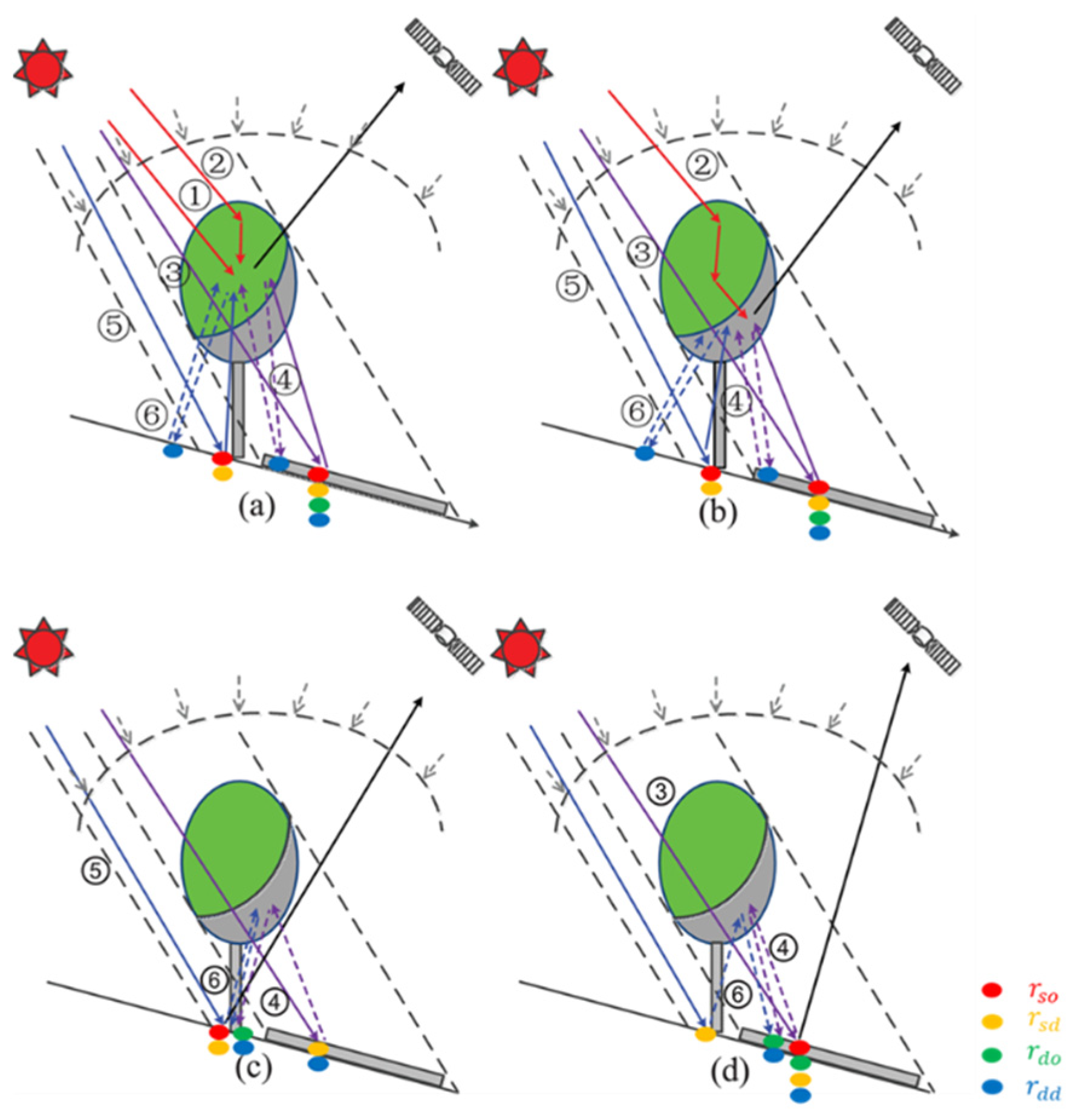
2.1.1. Four-Component BRFs Modeling with Only Direct Solar Radiation ($f_d=0$)

For $f_d=0$, only direct solar radiation with a certain incidence geometry exists in the scene. At this moment, four components of the forest canopy can be observed by sensor, namely sunlit crown, sunlit soil, shaded crown, and shaded soil. The reflected radiation of the four components in the forest canopy were parameterized according to the four-stream approximation algorithm [15]. Since the four-component BRFs all contain the interaction terms between photons and soil, the reflected radiation of soil can be divided into four four-stream reflected radiation (bi-directional, hemispherical-directional, directional-hemispherical, and bi-hemispherical reflected radiation), in consideration of the soil anisotropic reflected radiation during the parameterization. Figure 1 displays the reflected radiation transfer process of the four components in the forest canopy, in which each serial number represents a specific radiation transfer process. At the same time, the types of directional reflectance factors of the soil involved in the radiative transfer process are also marked with different colors (corresponding to different directional reflectance factors) in the diagram.

As for the sunlit crown (Figure 1a), the radiative transfer process of the sunlit crown included four cases: (1) single scattering from the crown without soil interactions (①); (2) multiple scattering from the crown without soil interactions (②); (3) photons transmitted through within-crown gaps (③ and ④); and (4) photons transmitted through between-crown gaps (⑤ and ⑥). The component BRF $C_s$, in the GOSAILT model (marked with $C_s^{old}$), was initially expressed as Equation (2), where the single variable $r_{soil}$ was used to describe the contribution of the soil reflectance to canopy BRF.

$$C_s^{old}={\rho }_{sos}+{\rho }_{sod}+\frac{\left[\left(1-P_{gap}\right)\left({\tau }_{ss}+{\tau }_{sd}\right)+P_{gap}\right]r_{soil}\left({\tau }_{oo}+{\tau }_{do}\right)}{1-r_{dd}\left(1-K_{open}\right){\rho }_{dd}}$$

(2)

where $P_{gap}$ represents the canopy gap ratio, and $K_{open}$ represents the canopy openness; ${\rho }_{sos}$ and ${\rho }_{sod}$ represent the single and multiple scattering of tree crown, respectively. $r_{soil}$ represents Lambertian soil reflectance. ${\tau }_{ss}$, ${\tau }_{sd}$, ${\tau }_{oo}$, and ${\tau }_{do}$ represent the bi-directional transmittance, hemispherical-directional transmittance, directional-hemispherical transmittance, and bi-hemispherical transmittance of tree crown, respectively.

Considering the soil reflectance anisotropy, the $r_{soil}$ in the Equation (2) is refined into four reflectance factors of soil: bi-directional reflectance ($r_{so}$), hemispherical-directional reflectance ($r_{do}$), directional-hemispherical reflectance ($r_{sd}$), and bi-hemispherical reflectance ($r_{dd}$); then, the $C_s$ is extended as the functions of four anisotropic soil reflectance factors (Equation (3)).

$$C_s={\rho }_{sos}+{\rho }_{sod}+\frac{\left[\left(1-P_{gap}\right)\left({\tau }_{ss}{r}_{so}+{\tau }_{sd}{r}_{do}\right)+P_{gap}{r}_{so}\right]{\tau }_{oo}+\left[\left(1-P_{gap}\right)\left({\tau }_{ss}{r}_{sd}+{\tau }_{sd}{r}_{dd}\right)+P_{gap}{r}_{sd}\right]{\tau }_{do}}{1-r_{dd}\left(1-K_{open}\right){\rho }_{dd}}$$

(3)

Similarly, according to the radiative transfer processes of Figure 1 and

Table A1. Radiative transfer processes of four scene components and relevant soil directional reflectance factors, under the condition of $f_d=0$.

Scene Component	ID	Radiative Transfer Processes	Soil Reflectance Factors
Sunlit crown	①	Solar photons→tree crown→sensor	—
	②	Solar photons→tree crown→(multiple scattering within tree crown)→sensor	—
	③	Solar photons→(within-crown gaps)→soil→tree crown→sensor	$r_{so}$, $r_{sd}$, $r_{do}$, $r_{dd}$
	④	Solar photons→(within-crown gaps)→soil→tree crown→soil→tree crown→sensor	$r_{dd}$
	⑤	Solar photons→(between-crown gaps)→soil→tree crown→sensor	$r_{so}$, $r_{sd}$
	⑥	Solar photons→(between-crown gaps)→soil→tree crown→soil→tree crown→sensor	$r_{dd}$
Shaded crown	②	Solar photons→tree crown→(multiple scattering within tree crown)→sensor	—
	③	Solar photons→(within-crown gaps)→soil→tree crown→sensor	$r_{so}$, $r_{sd}$, $r_{do}$, $r_{dd}$
	④	Solar photons→(within-crown gaps)→soil→tree crown→soil→tree crown→sensor	$r_{dd}$
	⑤	Solar photons→(between-crown gaps)→soil→tree crown→sensor	$r_{so}$, $r_{sd}$
	⑥	Solar photons→(between-crown gaps)→soil→tree crown→soil→tree crown→sensor	$r_{dd}$
Sunlit soil	④	Solar photons→(within-crown gaps)→shaded soil→tree crown→sunlit soil→sensor	$r_{sd}$, $r_{dd}$, $r_{do}$
	⑤	Solar photons→(between-crown gaps)→soil→sensor	$r_{so}$
	⑥	Solar photons→(between-crown gaps)→sunlit soil→tree crown→sunlit soil→sensor	$r_{sd}$, $r_{do}$, $r_{dd}$
Shaded soil	③	Solar photons→(within-crown gaps)→shaded soil→sensor	$r_{so}$, $r_{do}$
	④	Solar photons→(within-crown gaps)→shaded soil→tree crown→shaded soil→sensor	$r_{sd}$, $r_{dd}$, $r_{do}$
	⑥	Solar photons→(between-crown gaps)→sunlit soil→tree crown→shaded soil→sensor	$r_{sd}$, $r_{do}$, $r_{dd}$

, the other component BRF $G_s$, $T_s$, and $Z_s$ can be derived by following (Equations (4)–(6)).

$$G_s=r_{so}+\frac{\left[\left(1-P_{gap}\right)\left({\tau }_{ss}{r}_{sd}+{\tau }_{sd}{r}_{dd}\right)+P_{gap}{r}_{sd}\right]\left[\left(1-K_{open}\right){\rho }_{dd}\right]r_{do}}{1-r_{dd}\left(1-K_{open}\right){\rho }_{dd}}$$

(4)

$$T_s={\rho }_{sod}+\frac{\left[\left(1-P_{gap}\right)\left({\tau }_{ss}{r}_{so}+{\tau }_{sd}{r}_{do}\right)+P_{gap}{r}_{so}\right]{\tau }_{oo}+\left[\left(1-P_{gap}\right)\left({\tau }_{ss}{r}_{sd}+{\tau }_{sd}{r}_{dd}\right)+P_{gap}{r}_{sd}\right]{\tau }_{do}}{1-r_{dd}\left(1-K_{open}\right){\rho }_{dd}}$$

(5)

$$Z_s=\left(1-P_{gap}\right)\left({\tau }_{ss}{r}_{so}+{\tau }_{sd}{r}_{do}\right)+\frac{\left[\left(1-P_{gap}\right)\left({\tau }_{ss}{r}_{sd}+{\tau }_{sd}{r}_{dd}\right)+P_{gap}{r}_{sd}\right]\left[\left(1-K_{open}\right){\rho }_{dd}\right]r_{do}}{1-r_{dd}\left(1-K_{open}\right){\rho }_{dd}}$$

(6)

2.1.2. Four-Component BRFs Modeling with Only Atmospheric Diffuse Scattering ($f_d=1$)

For $f_d=1$, there is only atmospheric diffuse radiation and no shaded component in the forest canopy. In order to retain the same formats as those in direct illumination, the two components are split into a similar four components (i.e., $C_d$, $T_d$, $G_d$, and $Z_d$). In this case, the sunlit crown radiation of $C_d$ is consistent with that of shade crown radiation, $T_d$, and the sunlit soil radiation of $G_d$ is consistent with that of shade soil radiation, $Z_d$. Referring to Figure 1 and

Table A2. Radiative transfer processes of four scene components and relevant soil reflectance factors, under the condition of $f_d=1$.

Scene Component	ID	Radiative Transfer Processes	Soil Reflectance Factors
Sunlit crown/shaded crown	①	Solar photons→tree crown→sensor	—
	②	Solar photons→tree crown→(multiple scattering within tree crown)→sensor	—
	③/⑤	Solar photons→(within- and between-crown gaps)→soil→tree crown→sensor	$r_{do}$, $r_{dd}$
	④/⑥	Solar photons→(within- and between-crown gaps)→soil→tree crown→soil→tree crown→sensor	$r_{dd}$, $r_{do}$
Sunlit soil/shaded soil	③/⑤	Solar photons→(within- and between-crown gaps)→soil→tree crown→sensor	$r_{do}$
	④/⑥	Solar photons→(within- and between-crown gaps)→soil→tree crown→soil→sensor	$r_{dd},r_{do}$

, the quantities $C_d$, $G_d$, $T_d$, and $Z_d$ can be expressed as the functions of anisotropic soil reflectance factors (Equations (7) and (8)).

$$C_d=T_d={\rho }_{dos}+{\rho }_{dod}+\frac{\left[\left(1-K_{open}\right){\tau }_{dd}+K_{open}\right]\left(r_{do}{\tau }_{oo}+r_{dd}{\tau }_{do}\right)}{1-r_{dd}\left(1-K_{open}\right){\rho }_{dd}}$$

(7)

$$G_d=Z_d=\frac{\left[\left(1-K_{open}\right){\tau }_{dd}+K_{open}\right]r_{do}}{1-r_{dd}\left(1-K_{open}\right){\rho }_{dd}}$$

(8)

where ${\rho }_{dos}$ and ${\rho }_{dod}$ represent single and multiple scattering of the tree crown under the condition of pure sky light diffuse scattering, respectively.

2.2. Anisotropic Reflectance Factors of Soil

The simple soil directional (SSD) reflectance model is a two-parameter soil directional reflectance model, which is a simplification of Hapke model, based on radiative transfer theory, but has the similar simulation capability [16], which is expressed as follows:

$$r\left({\theta }_s,{\theta }_v,\phi ,\lambda \right)=\frac{{\rho }_0\left(\lambda \right)}{{\mu }_0+\mu }\left(\frac{e^{ag}}{1+g}-\frac{{\theta }_s{}^2+{\theta }_v{}^2}{10}\right)$$

(9)

where ${\rho }_0\left(\lambda \right)$ is the brightness parameter, varying with wavelength; $a$ is the direction-dependent shape parameter; and $r\left({\theta }_s,{\theta }_v,\phi ,\lambda \right)$ is the $r_{so}$ of four-component BRFs. The two terms, in the bracket of right side of the equation, denote the single and multiple scattering, respectively.

Theoretically, the hemispherical-directional reflectance ($r_{do}$), directional-hemispherical reflectance ($r_{sd}$), and bi-hemispherical reflectance factors ($r_{dd}$) can be solved by numerical integration of $r\left({\theta }_s,{\theta }_v,\phi ,\lambda \right)$, according to the following formula.

$$r_{do}\left({\theta }_v,\lambda \right)=\frac{1}{\pi }{{\displaystyle \int }}_0^{2\pi }{{\displaystyle \int }}_0^{\frac{\pi }{2}}r\left({\theta }_s,{\theta }_v,\phi ,\lambda \right)\sin {\theta }_s\cos {\theta }_{s}d{\theta }_{s}d\phi$$

(10)

$$r_{sd}\left({\theta }_s,\lambda \right)=\frac{1}{\pi }{{\displaystyle \int }}_0^{2\pi }{{\displaystyle \int }}_0^{\frac{\pi }{2}}r\left({\theta }_s,{\theta }_v,\phi ,\lambda \right)\sin {\theta }_v\cos {\theta }_{v}d{\theta }_{v}d\phi$$

(11)

$$r_{dd}\left(\lambda \right)=\frac{2}{\pi }{{\displaystyle \int }}_0^{\frac{\pi }{2}}{{\displaystyle \int }}_0^{2\pi }{{\displaystyle \int }}_0^{\frac{\pi }{2}}r\left({\theta }_s,{\theta }_v,\phi ,\lambda \right)\sin {\theta }_s\cos {\theta }_s\sin {\theta }_v\cos {\theta }_{v}d{\theta }_{v}d\phi d{\theta }_s$$

(12)

However, in order to avoid the over-complexity of the extended GOSAILT model and improve the efficiency of model operation, the empirical equations of $r_{do}$, $r_{sd}$, and $r_{dd}$ are derived by fitting the integral values simulated by the SSD model [16]. The results of the $r_{do}$, $r_{sd}$, and $r_{dd}$ empirical equations are highly consistent with the numerical integration results, which proves that the empirical equations of $r_{do}$, $r_{sd}$, and $r_{dd}$ are reliable enough to be used as inputs to the four-component BRFs model.

$$r_{do}\left({\theta }_v,\lambda \right)={\rho }_0\left(\lambda \right)c_1{e}^{c_{2}a}$$

(13)

where

$$\left\{\begin{array}{c}{c}_1=-0.037{\theta }_v{}^2+0.006{\theta }_v+0.297\\ c_2=0.763{\theta }_v{}^2-0.130{\theta }_v+0.924\end{array}\right.$$

(14)

And,

$$r_{sd}\left({\theta }_s,\lambda \right)={\rho }_0\left(\lambda \right)c_1{e}^{c_{2}a}$$

(15)

where

$$\left\{\begin{array}{c}{c}_1=-0.037{\theta }_s{}^2+0.006{\theta }_s+0.297\\ c_2=0.763{\theta }_s{}^2-0.130{\theta }_s+0.924\end{array}\right.$$

(16)

Besides,

$$r_{dd}\left(\lambda \right)=0.270{\rho }_0\left(\lambda \right)e^{1.446a}$$

(17)

3. Datasets

The UAV multi-angle BRF observation and DART simulation BRF datasets were used to evaluate the accuracy of GOSAILT-SSD model. Since grounded multiangular BRF observations of mountain forest are difficult to obtain, the UAV multi-angle BRF dataset was obtained over flat land surface, and the DART simulation dataset covered various topographic conditions.

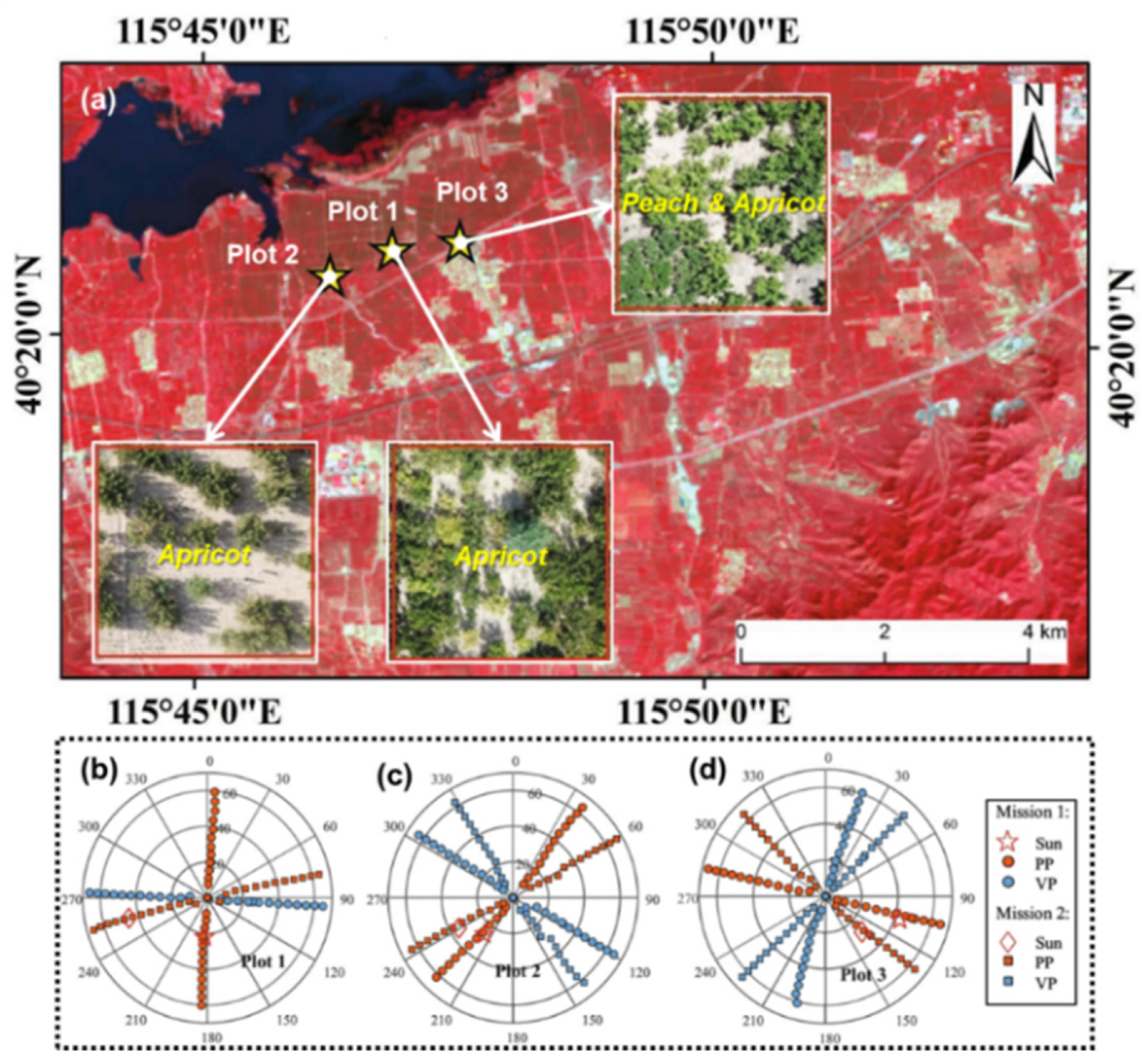
3.1. UAV-Observed BRF Dataset

The targets of UAV observation dataset are three sample plots, located in the rural area (40.34° N, 115.78° E) of Huailai County, Hebei Province, China, which are in a flat terrain with a subhumid continental climate and an altitude of 480~485 m (Figure 2a). Three sample plots are typical orchards of northern China, and their background is bare, dry clay (soil moisture content is less than 18%, and clay content on the top layer of soil is around 60–75%). The dataset was acquired on 30–31 July 2019. During the experiment, the weather was clear, with no wind or clouds. Two observations (i.e., Mission 1 and Mission 2) were implemented for each sample plot (Figure 2b–d). The UAV used in the experiment was the DJI M600 pro (DJI Technology Co., Ltd., Shenzhen, China), on which a multispectral camera (MAPIR survey 3 NRGN, manufactured by Peau Productions, Inc., San Diego, CA, USA) with three narrow spectral bands (central wavelengths of 550, 660, and 850 nm) was loaded. The detailed scheme about UAV observation experiment can be referred to the literature [10]. Besides, canopy structure properties (vegetation coverage, LAI, crown diameter and so on), leaf spectral profile and soil BRF profile of each plot were also observed.

Radiometric calibration, geometric correction, and multiangular information extraction (including illumination geometry, observation geometry, and BRF) were carried out for each UAV image acquired in the field, so as to obtain the multiangular BRF dataset, under the conditions of two illumination geometry, for each sample plot. For each illumination geometry, each sample plot contains multiangular observation, with an VZA interval of 5° from −60°(backward-scattering) to 60° (forward-scattering) in the solar principal plane (PP). A more detailed flowchart on calculating UAV BRF can be founded in the work of Li et al. [10]. In the model evaluation with the UAV dataset, the two parameters in soil anisotropic reflectance factors of the GOSAILT-SSD model were inversed optimally using the UAV-derived soil BRF profile of each sample plot (see

Table 1. GOSAILT-SSD parameters, corresponding to the UAV multi-angle observations.

Input Parameters		Unit	Plot 1	Plot 2	Plot 3
Spectral properties (850 nm)	Leaf reflectance	[-]	0.449	0.477	0.455
	Leaf transmittance	[-]	0.449	0.477	0.455
	$\mathrm{SSD}\mathrm{parameter}({\rho }_0$)	[-]	0.62	0.65	0.64
	$\mathrm{SSD}\mathrm{parameter}(a$)	[-]	0.17	0.31	0.32
Canopy structural properties	Tree density	[hr−1]	646	456	883
	LAI	[m2/m2]	2.36	1.71	2.83
	Coverage	[%]	58	34	62
	Crown vertical axis	[m]	1.44	1.13	1.01
	Crown horizontal axis	[m]	1.69	1.54	1.5
	Canopy height	[m]	1.93	1.78	1.56
	Leaf dimension	[m]	0.2	0.2	0.2
Topographic	Slope	[°]	0	0	0
	Aspect	[°]	0	0	0
Atmospheric	SKYL	[-]	0	0	0
Illumination-observation geometry	SAA (Massion 1)	[°]	184.21	218.22	134.44
	SZA (Massion 1)	[°]	23.5	30.8	33.5
	SAA (Massion 2)	[°]	255.47	240.66	107.34
	SZA (Massion 2)	[°]	45.5	42.8	48.5
	VAA	[°]	PP	PP	PP
	VZA	[°]	0–60	0–60	0–60

), and the Lambertian soil reflectance in the original GOSAILT model was set a constant value of the nadir view direction, simulated by the SSD.

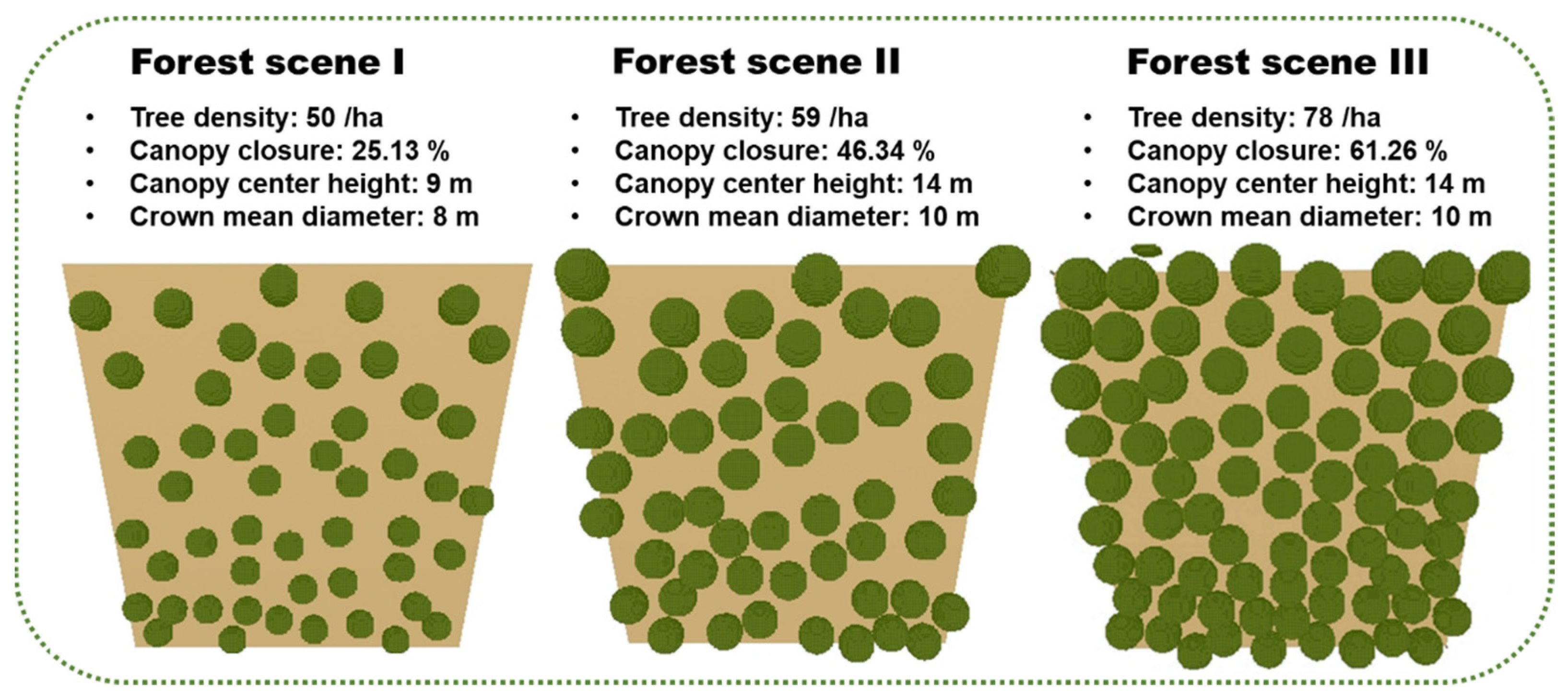
3.2. DART-Simulated BRF Dataset

The DART (discrete anisotropic radiative transfer) model is one of the computer simulation models, which can simulate the anisotropic reflection characteristics of complex 3-D scenes at pixel scale [28]. Here, it was used as a benchmark to evaluate the accuracy of BRDF model, considering anisotropic background soil reflectance for a mountain forest. The area of the forest scene was set as 100 m × 100 m, the leaf area index (LAI) of a single tree crown was set as 4, and the tree crown was uniformly distributed in the scene. Three kinds of forest canopies (including 50, 59, and 78 trees) were set, corresponding to three different crown densities (see Figure 3). For each forest canopy with specific density, a further 49 scenes were constructed, according to its topographic slope changing from 0° to 60° and SZA changing from 0° to 60°. Therefore, a total of 147 forest scenarios were constructed using the DART simulation system, covering different crown densities, topographies, and SZAs. For each forest scene, both the topographic aspect and solar azimuth angle (SAA) were set to a fixed value of 0°, while the observation geometry (VZA and VAA) remained with 50 default values of DART; that is, the observation geometry positions were uniformly distributed in the hemispheric ($2\pi$) space.

The setting of spectral parameters mainly involves leaf reflectance, leaf transmittance, and soil reflectance in red and near-infrared (NIR) spectral bands. As with the GOSAILT model, the leaves were still treated as Lambertian reflectors, with reflectance and transmittance varying only in wavelength. Background soil was treated as an anisotropic reflector in this study, and its anisotropy was described by the five parameters Hapke model (

Table 2. Canopy spectral parameter settings of the DART.

Object	Parameters	Red Band	NIR Band	Data Source
Leaf	reflectance	0.055	0.496	GOSPEL spectral library [7]
	transmittance	0.015	0.441
Soil	$\omega$	0.5106	0.5434	Zeng et al. [29]
	$b$	0.82	0.86	Default Hapke parameters of for a typical plowed field [18]
	$c$	0.67	0.70
	$B_0$	0.30	0.33
	$h$	0.25	0.21
	$a$	0.0720	0.0614

) in the DART software (version 5.7.0). There are 294 groups of forest canopy multi-angular reflectance data (uniformly distributed in hemispheric space) in the DART simulation dataset, including the red and NIR bands, and each group of data covers 50 observation directions in hemispheric space. The reflectance output of the DART software employed in the simulation experiment is the reflectance based on the definition of horizontal incident energy; thus, the cosine correction method was used to convert the reflectance simulated by DART into slope reflectance [7], which is then used as the reference truth value to evaluate the model. In the model evaluation with the DART dataset, the two parameters in the soil anisotropic reflectance factors of GOSAILT-SSD model were inversed optimally using the DART-simulated soil BRF profile, and the Lambertian soil reflectance in the original GOSAILT model was set a constant value of the nadir view direction, simulated by the SSD model (shown in Figure 4).

4. Results

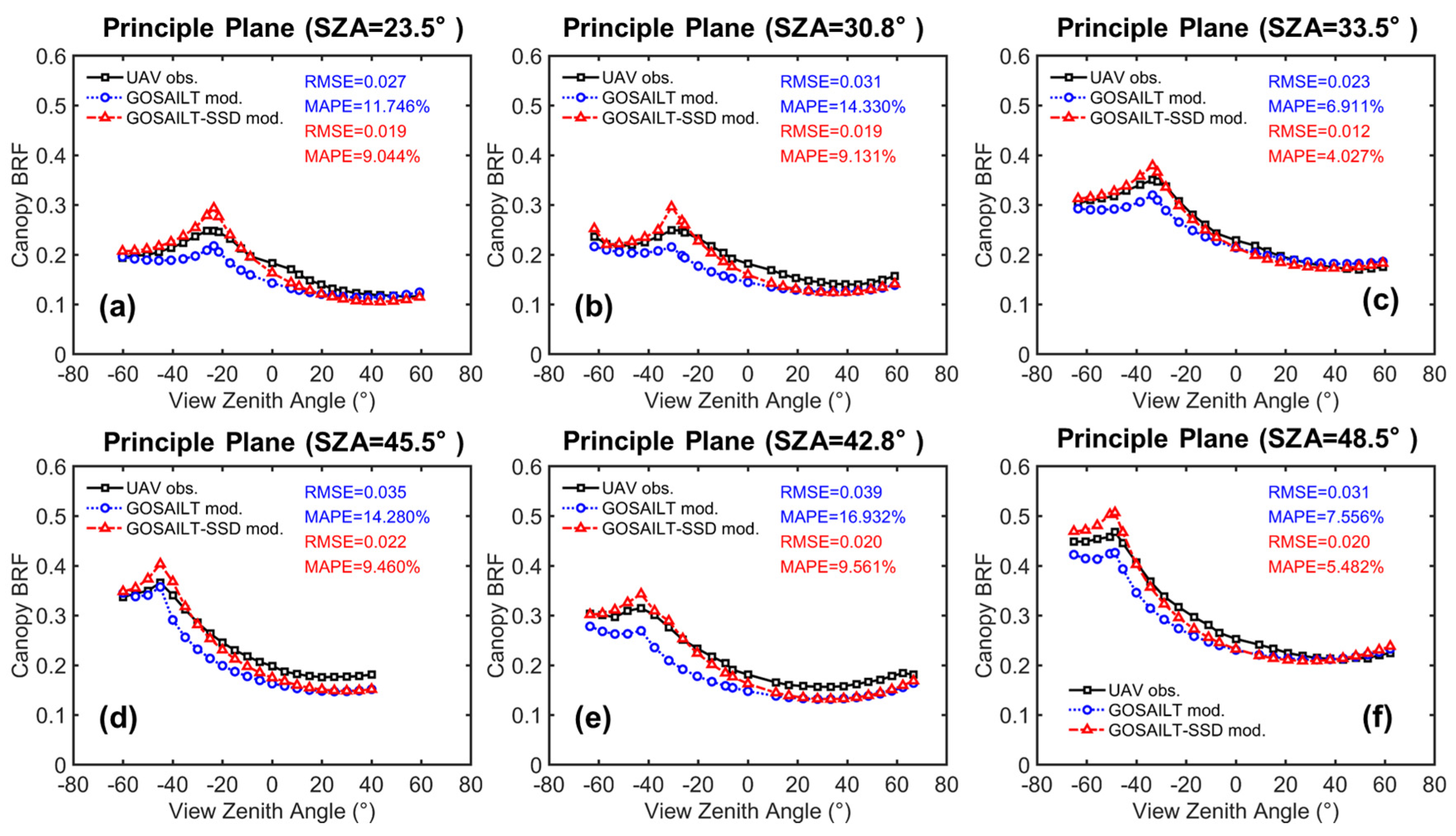
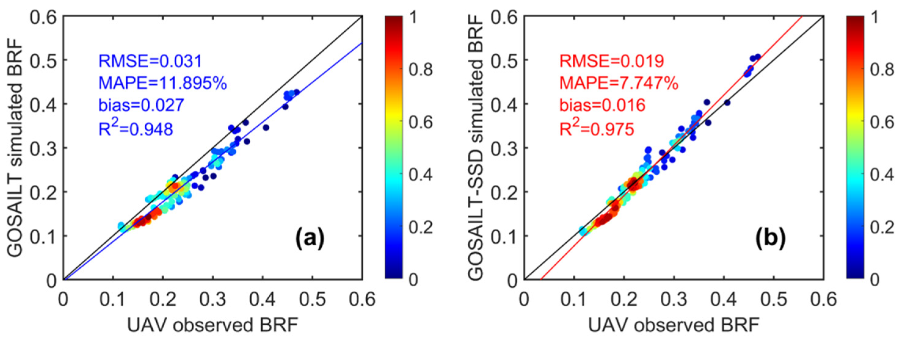
4.1. Validation with UAV-Observed BRF

As shown in Figure 5, the UAV multi-angular observations are used to further evaluate the modified GOSAILT (GOSAILT-SSD) model. The fruit-plantation canopy BRF in the PP, observed by the UAV, is asymmetric in the NIR band, showing an obvious bowl shape. The higher and lower BRF correspond to the backward-scattering (VZA < 0) and forward-scattering directions (VZA > 0), respectively, and the canopy BRF in the hot spot direction reaches the maximum. With the increase of SZA, the bowl shape of the canopy BRF is more obvious, and the BRF in the backward-scattering direction is larger. Compared with the UAV observations, the original GOSAILT underestimates the BRF near the hotspot directions, while the GOSAILT-SSD simulations show similar shape patterns, which indicates the GOSAILT-SSD can improve the BRF simulations (especially near the hotspot directions). Meanwhile, the improvement degree of the canopy BRF simulations by the GOSAILT-SSD varies with the fraction of vegetation cover and SZA, which is because different fractions of vegetation cover or SZAs can lead to the areal proportion differences of sunlit soil. For example, with the GOSAILT-SSD, the BRF simulations RMSE (MAPE) of sparse canopy in Plot-2 are decreased from 0.039 (16.932%) to 0.020 (9.561%) (see Figure 5e), while the RMSE (MAPE) of dense canopy in Plot-3 are decreased from 0.031 (7.556%) to 0.020 (5.482%) (see Figure 5f). Although the differences exist, a higher overall accuracy of the GOSAILT-SSD model is shown, which underlines the significance of coupling the SSD to the GOSAILT to model canopy BRF of fruit-plantation with anisotropic soil reflectance.

Figure 6 shows the total scatterplot and statistical results of all scenarios simulated by the GOSAILT and GOSAILT-SSD model. The results suggest that the GOSAILT-SSD can improve the directional reflectance simulations in the NIR band, leading to a higher accuracy, compared with original GOSAILT simulations, which neglects reflectance anisotropy of soil. With the GOSAILT-SSD model, the fitting line of scatterplot is close to the 1:1 line, and all accuracy indexes are improved (RMSE = 0.019, MAPE = 7.7%, bias = 0.016, R² = 0.97). This means that simulations of the GOSAILT-SSD model are broadly in line with the field observations, and the GOSAILT-SSD model has a good performance for directional reflectance simulations of artificial forest canopy on flat surface.

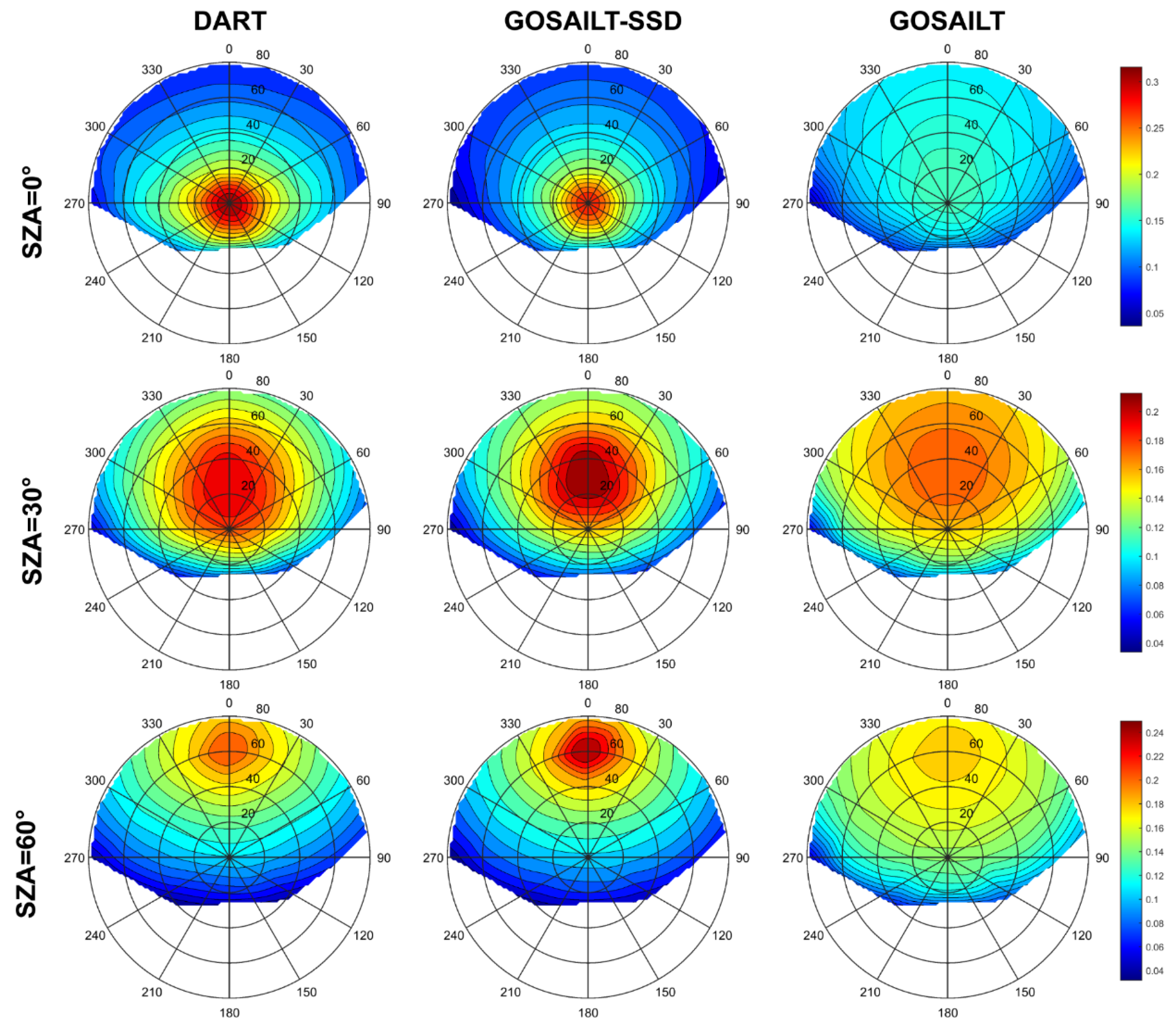
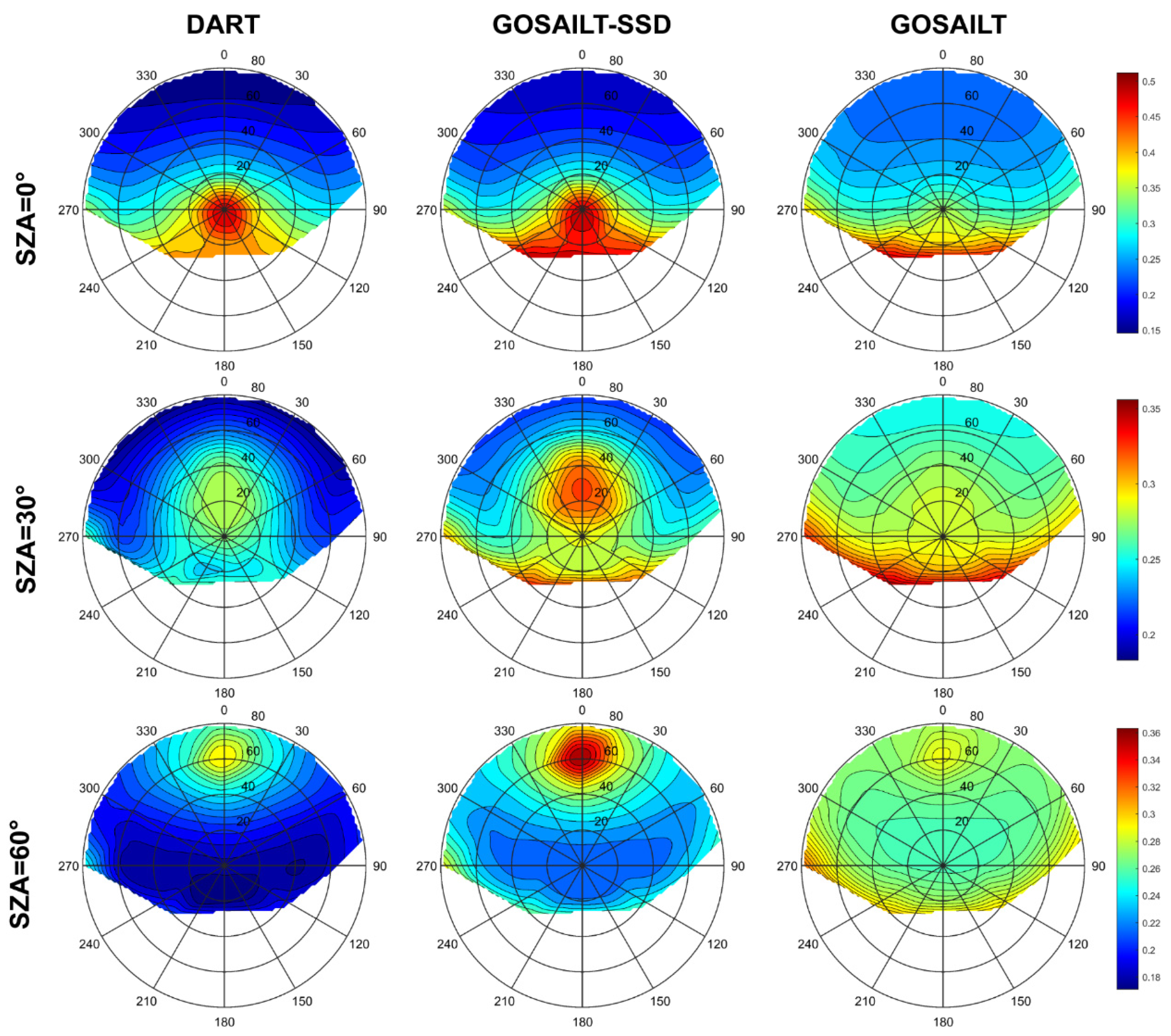
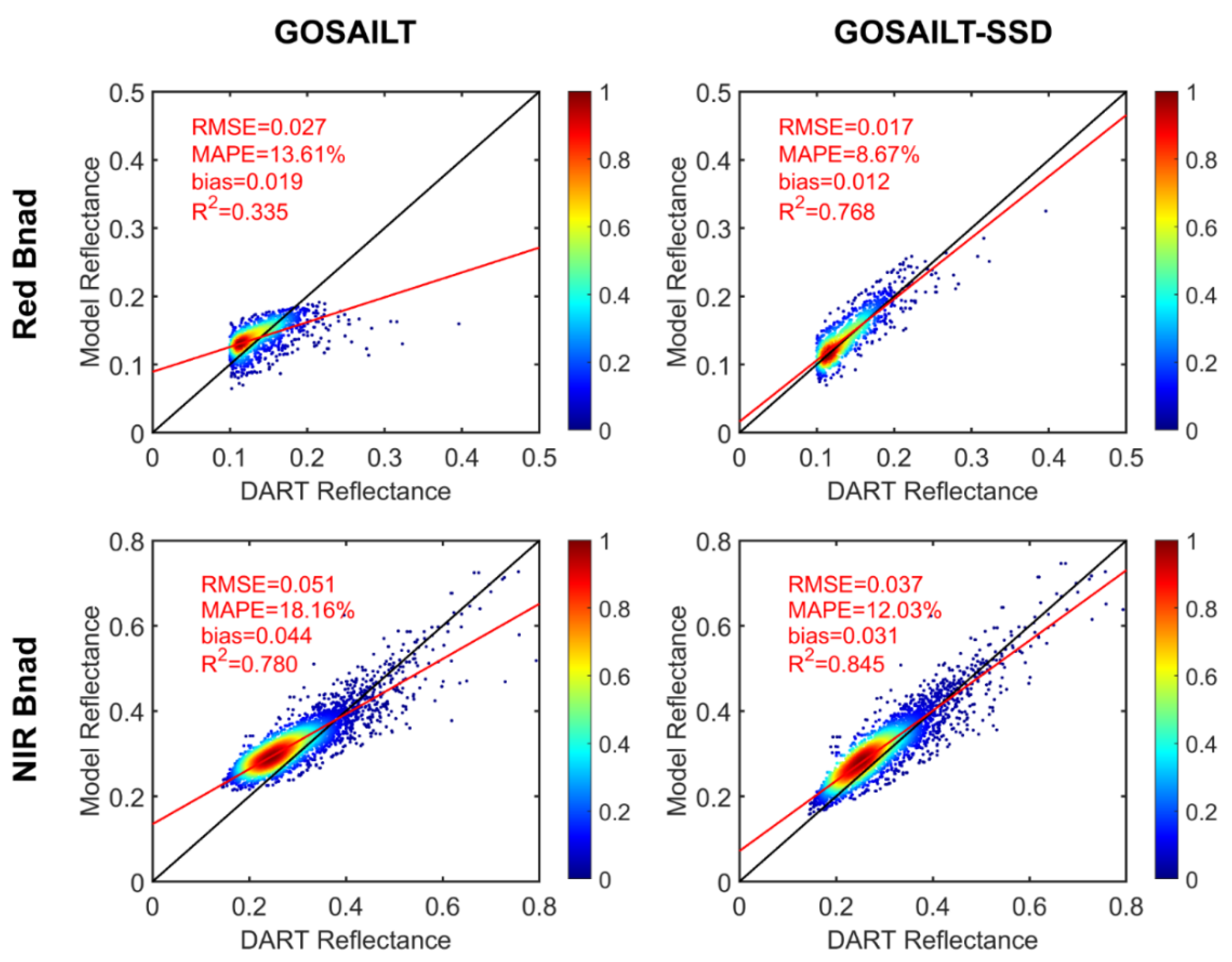
4.2. Validation with DART-Simulated BRF

As shown in Figure 7, the GOSAILT-SSD simulated BRFs in the red band are compared with the DART-simulated reflectance. As it can be seen, both the GOSAILT-SSD and original GOSAILT show a larger BRF in the solar illumination direction, but the latter has a larger BRF value and more significant hot spot effect. Compared with the BRFs simulated by DART, the original GOSAILT model shows BRF underestimation in the observation direction of the high-BRF region (near the hot spot direction) and observation direction of low-BRF region (forward-looking direction), and this phenomenon is more obvious when the SZA is small. However, the GOSAILT-SSD model shows a better agreement with the reference BRFs by DART simulation, which can better describe the hot spot effect and BRDF characteristics (shape) of canopy BRF in mountain forest. These results indicate that the GOSAILT-SSD model with non-Lambertian soil has high accuracy in the red band.

Similarly, the results of the comparison in the NIR band are shown in Figure 8. It can be found that, when SZA is small, the original GOSAILT cannot describe the hot spot effect of forest canopy BRF, and the maximum BRF appears in the forward-scattering direction. Although the hot spot effect of BRF is captured with the increase of SZA, there is a serious underestimation, compared with the DART simulation, which is consistent with the phenomenon of that in the red band. However, the GOSAILT-SSD model can better describe the hot spot effect of mountain forest canopy BRF in the NIR band, and anisotropic characteristics of the simulated BRF are in good agreement with the reference BRF by DART. Compared with the original GOSAILT, which does not consider the non-Lambertian reflection characteristics of soil, the GOSAILT-SSD model can significantly improve the simulation performance.

The performance of the GOSAILT-SSD under different topographic conditions and canopy density was further evaluated, and it was found that the model could accurately describe the anisotropic characteristics of forest canopy BRF under different topographic conditions and canopy density levels. Figure 9 shows the overall accuracy of the GOSAILT and GOSAILT-SSD. In the mountain forest canopy with rough soil background, the RMSE, MAPE, bias, and R² of the original GOSAILT model for canopy BRF simulation of red band were 0.027, 13.61%, 0.019, and 0.335, respectively. The corresponding accuracy indexes of NIR band were 0.051, 18.61%, 0.044, and 0.780, respectively. However, the accuracy of the modified model was significantly improved, and RMSE, MAPE, bias, and R² for the red band were 0.017, 8.67%, 0.012, and 0.768, respectively; those of NIR band were 0.037, 12.03%, 0.031, and 0.845, respectively. These results indicate that the GOSAILT-SSD performs well in mountain forest with rough soil because it considers the anisotropy of soil reflectance. On the other hand, the GOSAILT shows considerably worse results over the same scene, which manifests that it is not enough to consider only the anisotropy of tree crown reflectance to describe the BRF of canopy in the mountain forest with rough soil, but the anisotropy of soil reflectance should be considered.

5. Discussion

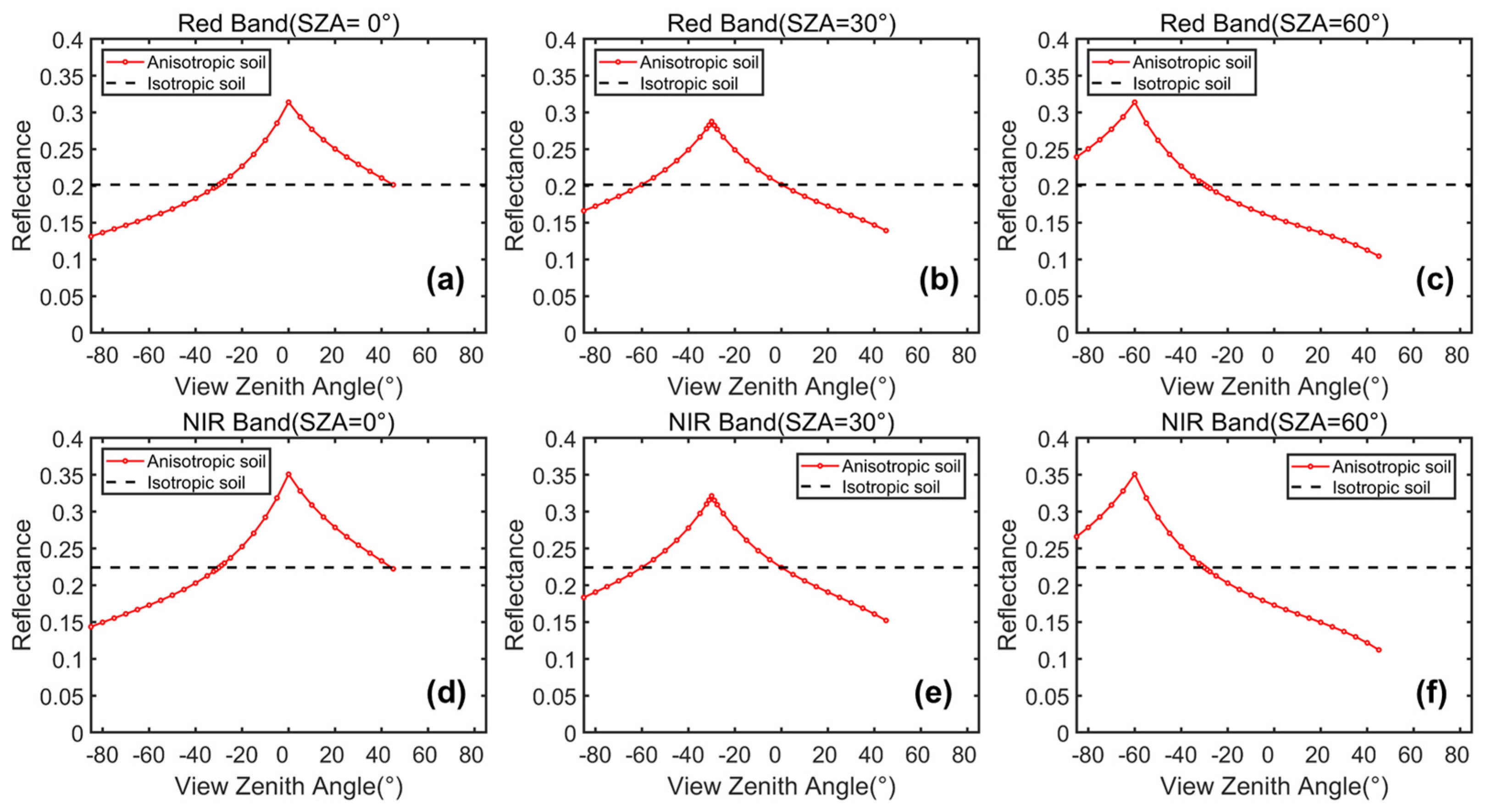
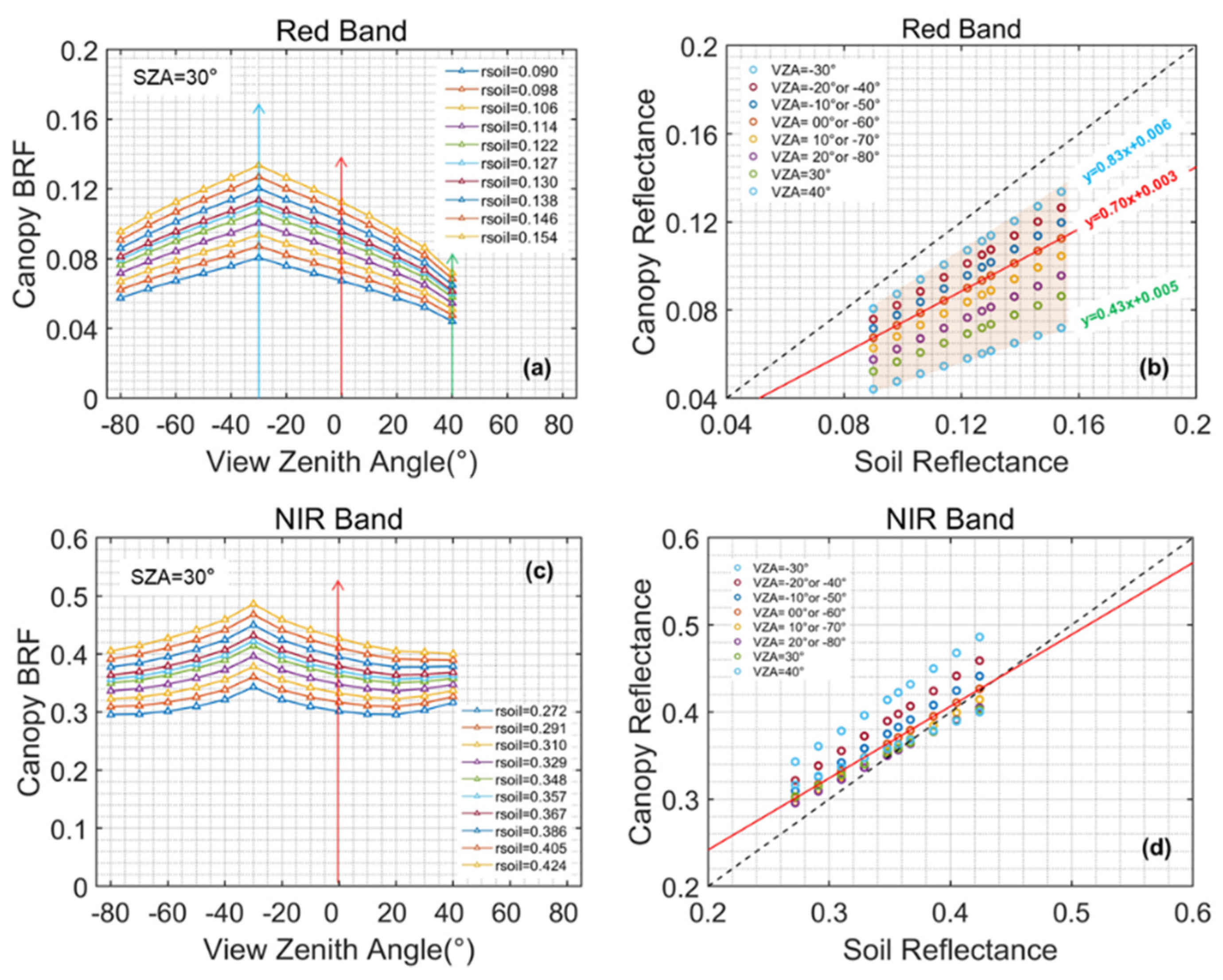
5.1. Sensitivity of Forest Canopy BRF to Soil Reflectance

Soil reflectance is an important driving variable of forest canopy BRDF model. The local sensitivity analysis of soil reflectance was performed with the original GOSAILT model, and it was found that forest canopy BRF, under all VZA conditions in the PP, increased with the increase of soil reflectance (Figure 10a,c). Meanwhile, the canopy BRF showed a perfect linear relationship with soil reflectance (Figure 10b,d). Here, the slope of the regression line can be expressed as $\Delta BR{F}_{Canopy}/\Delta r_{soil}$, so the slope of regression line is used to quantitatively characterize the contribution of soil reflectance to canopy BRF. The slope of regression line varies from 0 to 1, which means the contribution of the soil reflectance varies from 0% to 100%. As shown in Figure 10b, in terms of the red band, the slope of the regression line varies with VZA, with the maximum (0.83) and minimum (0.43) corresponding to the hot and cold spot directions, respectively, and the slope of the nadir direction is 0.7. The slope of the regression line, under most VZA conditions, is greater than 0.6 in the red band. For the NIR band, it had similar results (Figure 10d). The results suggest that the contribution of soil reflectance to canopy BRF is large (more than 60%) for sparse canopy (Cv = 25.13%). The local sensitivity analysis results demonstrate the importance of soil reflectance for canopy BRF and show that soil reflectance is an important and highly-sensitive driving variable for the discrete forest canopy BRDF model over a sloped surface. Therefore, in addition to topography, the accurate description of soil reflectance should not be ignored in BRDF modeling for discrete forest canopy.

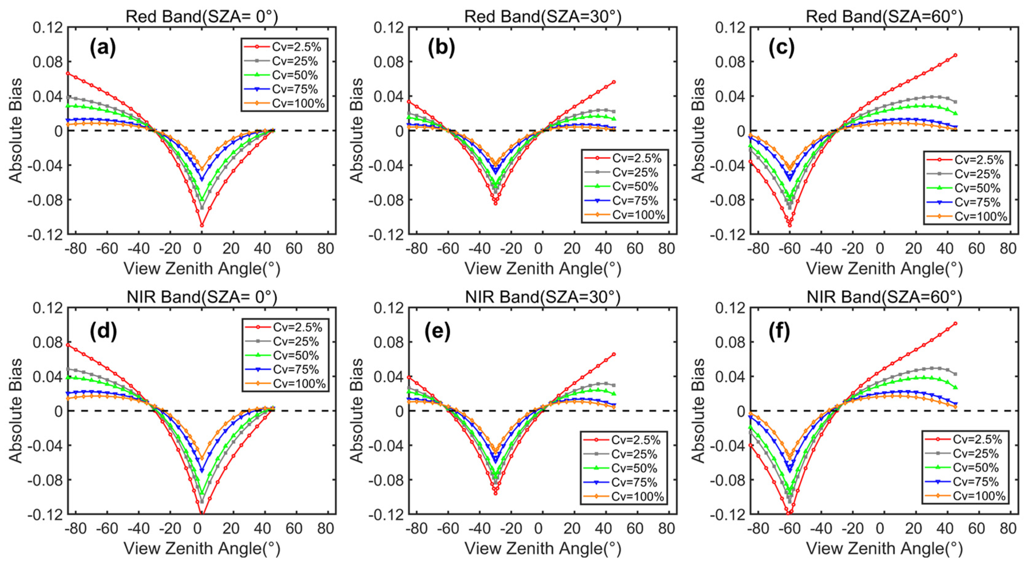
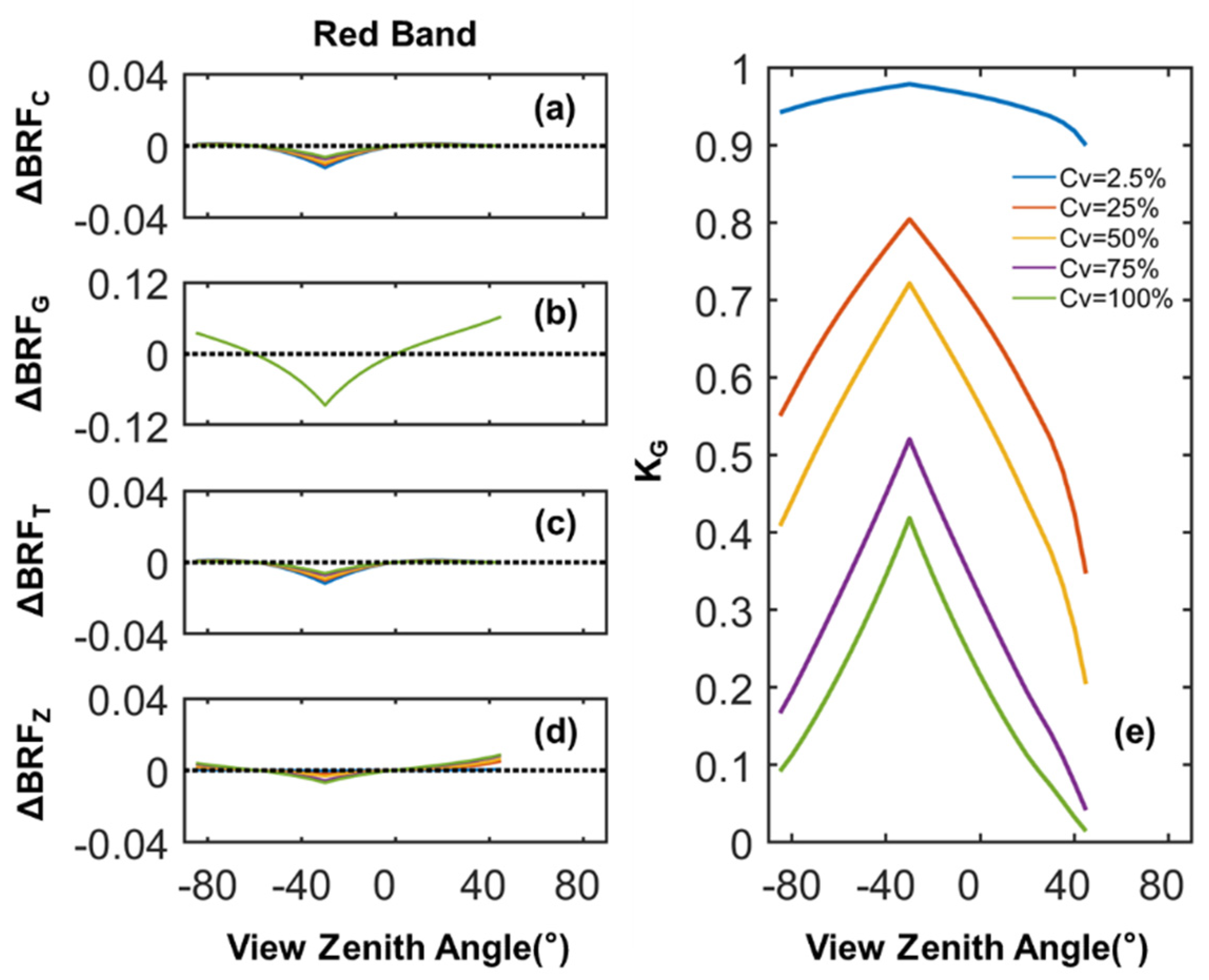
5.2. Impact of Soil Reflectance Anisotropy on Forest Canopy BRF Characteristics

To characterize the impacts of soil anisotropy on forest canopy BRF characteristics, the canopy BRF profiles of various virtual forest scenes were firstly simulated using GOSAILT and GOSAILT-SSD; then, the discrepancies of canopy BRF between isotropic and anisotropic soil conditions (shown in Figure 4) were analyzed under different fractions of vegetation cover (Cv), view zenith angles (VZA), incident solar zenith angles (SZA), and spectral bands. The setting of canopy other structural and spectral parameters was the same as that in Section 3.2. The absolute deviation ($AD=BR{F}_{vi}^{GOSAILT}-BR{F}_{vi}^{GOSAILT-SSD}$) at a given view direction between the GOSAILT and the GOSAILT-SSD was used to estimate canopy BRF discrepancies.

(1) Fraction of vegetation cover: Five types of forest scenes with different tree-crown densities are set to control the fractions of vegetation cover (Cv), including 2.5%, 25%, 50%, 75%, and 100%. By comparing the canopy BRF error of Lambertian soil assumption under different Cv levels in Figure 11, it can be found that the smaller the Cv, the more significant the absolute bias is (except for some specific VZA), which is because the smaller the Cv, the larger the area proportion of soil observed (Figure 12b), resulting in the absolute bias of forest canopy BRF larger. However, as for some specific VZA, where all lines converge to the same point (e. g. VZA = 0° in Figure 11b), there is no discrepancy among different Cv levels, which is because Lambertian soil assumption does not cause four-component BRF errors in these VZA conditions (Figure 12a). As shown in Figure 11b, when the SZA is 30° and VZA is 30°, the BRF absolute bias of forest canopy with Cv = 25% in the red (NIR) band is −0.071 (−0.083), while the BRF absolute bias of forest canopy with Cv = 100% is −0.04 (−0.048). Since the GOSAILT model assumes that the tree crown is spherical and randomly distributed in the scene, sunlit soil can still be observed when the forest Cv increases to 100% (Figure 12b), leading to canopy BRF errors not equal to 0.

(2) View zenith angles: The canopy BRF errors of Lambertian soil assumption differ from the view zenith angles along the PP. As shown in Figure 11b, for forest canopy with Cv = 25% and SZA = 30°, when the VZA are −60° and −30°, the corresponding absolute biases of red band are 0 and −0.071, respectively. When the VZA are +30° and +45°, both absolute biases are 0.022 (see

Table 3. Forest canopy reflectance error statistics under different spectral bands (SZA = 30°).

VZA	Cv = 25% (Sparse Forest)				Cv = 100% (Dense Forest)
(°)	ADred	ADnir	RDred	RDnir	ADred	ADnir	RDred	RDnir
−85	0.02	0.027	20.4%	14.8%	0.004	0.01	11.1%	3.2%
−60	0	0.002	0.0%	0.1%	0	0.005	0.6%	1.5%
−30	−0.071	−0.083	−29.1%	−26.3%	−0.04	−0.048	−21.8%	−10.0%
0	0	0.002	0.0%	0.1%	0	0.005	0.6%	1.5%
30	0.022	0.029	24.8%	16.5%	0.004	0.01	12.1%	2.9%
45	0.022	0.03	40.2%	9.8%	0.001	0.004	10.8%	1.2%

Note: VZA < 0 denotes backward-scattering direction, VZA > 0 denotes forward-scattering direction; AD_red and AD_nir indicate the absolute deviation in the red and NIR bands, respectively, while RD_red and RD_nir indicate the relative deviation in the red and NIR bands, respectively. The relative deviation is expressed as: $RD=AD/BR{F}_{vi}^{GOSAILT-SSD}\times 100\%$.

). The results indicate that the Lambertian soil assumption can cause underestimation and overestimation of forest canopy BRF; the most serious underestimation occurs in the direction of hot spot effect, and the most serious overestimation occurs in the direction of forward-scattering. This is because the reflectance of real soil is anisotropic and has weak forward-scattering, as well as strong backward-scattering (especially in the direction of hot spot effect). When the VZA is 0°, the absolute bias is 0, which means there is no deviation in canopy BRF, due to the correct value of soil BRF in the nadir view direction. Meanwhile, at other VZA (e.g., VZA = −60° in Figure 11b, where all lines also converge to the same point), the absolute bias of canopy BRF is also 0. This occurs because the value of anisotropic soil reflectance, under these VZA conditions, is exactly equal to the value of isotropic soil reflectance (see Figure 4b), resulting in the unbiasedness of canopy BRF.

(3) Solar zenith angles: The incident solar zenith angle changes the angular distribution of canopy reflectance by changing the area proportion and BRF shape of four components, especially the area proportion and BRF shape of sunlit soil. Canopy BRF error at different incident zenith angles are generated, including 0°, 30°, and 60°. As shown in Figure 11a–c, for forest canopy with Cv = 2.5%, when the SZA are 0°, 30°, and 60°, the corresponding absolute biases of hotspot observation direction in the red band are −0.110, −0.084, and −0.110, respectively. Meanwhile, for forest canopy with Cv = 25%, the corresponding absolute biases are of −0.09, −0.07, and −0.09, respectively. These results indicate that the absolute biases of canopy BRF at SZA = 30° are smaller than those of at SZA = 0° and SZA = 60°, especially for sparser canopy. This is mainly because the BRF error of sunlit soil is the smallest, and the area proportion of sunlit soil is large enough for sparser canopy, when the SZA is 30° over a sloping terrain of slope = 30°.

(4) Spectral bands: Comparing Figure 11a–c with Figure 11d–f, it can be found that there are differences in the canopy BRF error between the red and NIR bands. Under the same Cv, VZA, and SZA conditions, the absolute bias in the NIR band is slightly larger than that of the red band, but the relative bias is smaller than that of the red band, especially for the forest scene with larger Cv. For example, as shown in Figure 11b,e and Table 3, when the Cv is 25% and VZA is −30° (backward-scattering direction), the absolute bias is −0.071 (underestimated by 29.1%) in the red band, while the absolute bias is −0.083 (underestimated by 21.8%) in the NIR band. Under the same observation geometry, for forest canopy with Cv = 100%, the absolute bias is −0.04 (underestimated by 26.3%) in the red band, and the absolute bias is −0.048 (underestimated by 10%) in the NIR band. The results occur since vegetation is brighter than soil in the NIR band; meanwhile, stronger multi-scattering of canopy moderates the impact of soil reflectance anisotropy on canopy BRF.

6. Conclusions

The anisotropy of soil reflectance is a significant source of uncertainty in BRF simulation of sparse woodland. In order to reduce this uncertainty, the GOSAILT model is extended and improved by coupling the background soil’s non-Lambertian reflectance characteristic function, in order to develop the GOSAILT-SSD model. Thus, the GOSAILT-SSD model could take the topographic effect, tree’s geotropic nature, atmospheric diffuse-scattering, and soil anisotropic reflectance of mountain forest into account. The accuracy of the GOSAILT-SSD model was validated by employing UAV field multi-angular observations and DART simulations. The results indicate that the GOSAILT-SSD model exhibits good performance for woodland canopy BRF simulations. The validation with UAV field multi-angle observation data shows high accuracy with RMSE (MAPE, Bias, and R²), corresponding to 0.019 (7.7%, 0.016, and 0.97) for canopy BRF simulation of orchards over flat surfaces. The validation with DART simulation data shows that the RMSE (MAPE, Bias, and R²) of the GOSAILT-SSD model in the red and NIR bands are 0.017 (8.67%, 0.012, and 0.768) and 0.037 (12.03%, 0.031, and 0.845), respectively. The results indicate that, in addition to the topography effects, the anisotropy of soil reflectance should also be emphasized in BRDF modeling for discrete woodland. To the best of our knowledge, GOSAILT-SSD is the only one physical BRDF model over sloping terrain that has soil anisotropic reflectance considered, so far.

Then, the sensitivity of canopy BRF to soil reflectance and the impact of soil reflectance anisotropy on forest canopy BRF characteristics were analyzed, based on a series of GOSAILT and GOSAILT-SSD model simulations. It is found that the forest canopy BRF is highly sensitive to soil reflectance. The BRF simulation accuracy of mountain forest canopy is significantly affected by the Lambertian soil approximation, and there are differences in the effect among different fractions of vegetation cover, different VZAs, different SZAs, or different spectral bands. The canopy BRF error, caused by the Lambertian soil approximation, decreases with the increase of fraction of vegetation cover. In the solar principal plane, the Lambertian soil approximation results in a severe underestimation of BRF in the hot spot direction and an obvious overestimation in the large observation zenith angles. The absolute error caused by the Lambertian soil approximation in the NIR band is slightly larger than that of the red band, but the relative error in the red band is larger than that of the NIR band. The results corroborate earlier findings, especially those by Privette et al. [14] and Li et al. [10], who have carried out similar studies, regarding error analysis of Lambertian soil assumption, based on computer simulation models. As the results show in this study, the canopy reflectance is largely biased, due to the Lambertian soil assumption. If the canopy BRDF model, ignoring the soil reflectance anisotropy, is used to retrieve canopy structural parameters (e.g., LAI and clumping index) and leaf functional traits (e.g., foliar chlorophyll content and leaf mass per area), it will cause large retrieval errors. The findings presented in this research can be used to analyze the propagation mechanism of leaf functional and canopy structural trait retrieval errors, due to the Lambertian soil assumption in the BRDF model, further finding a better strategy for the estimation of leaf functional and canopy structural traits, based on regular spectral measurements.

However, some limitations still exist in our study, such as the spheroidal crown shape implication in the GOSAILT model [30], uncertainty of the SSD model, simplification of forest background in the real world, and so on. Taking bare soil as an example, this paper considers the anisotropy of background reflectance in the BRDF model of mountain forest canopy. In the real world, the forest background can also be dense grassland or a combination of weeds, lichens, moss, litter, or even snow in the winter boreal [10,31]. For these cases, it is only needed to couple the corresponding background anisotropic reflectance characteristic function into the extended GOSAILT model of this paper. For example, the anisotropic reflectance characteristic function of grassland can be derived by using the kernel-driven RTLSR model [32] or physical PROSAIL model [33], and the anisotropic reflectance characteristic function of snow can be deduced by using the kernel-driven snow BRDF model [34]. In the future, the method proposed in this paper will be further evaluated and sequentially employed to couple the background grassland’s non-Lambertian reflectance characteristic function, in order to develop tree–grass ecosystem BRDF models over a sloped surface.

References

1. Schaepman-Strub, G.; Schaepman, M.E.; Painter, T.H.; Dangel, S.; Martonchik, J.V. Reflectance quantities in optical remote sensing—definitions and case studies. Remote Sens. Environ. 2006, 103, 27–42. [Google Scholar] [CrossRef]
2. Hao, D.; Wen, J.; Xiao, Q.; Wu, S.; Lin, X.; You, D.; Tang, Y. Modeling Anisotropic Reflectance Over Composite Sloping Terrain. IEEE Trans. Geosci. Remote Sens. 2018, 56, 3903–3923. [Google Scholar] [CrossRef]
3. Bacour, C.; Bréon, F.-M.; Maignan, F. Normalization of the directional effects in NOAA–AVHRR reflectance measurements for an improved monitoring of vegetation cycles. Remote Sens. Environ. 2006, 102, 402–413. [Google Scholar] [CrossRef]
4. Vanonckelen, S.; Lhermitte, S.; Van Rompaey, A. The effect of atmospheric and topographic correction methods on land cover classification accuracy. Int. J. Appl. Earth Obs. Geoinf. 2013, 24, 9–21. [Google Scholar] [CrossRef] [Green Version]
5. Wen, J.; Liu, Q.; Xiao, Q.; Liu, Q.; You, D.; Hao, D.; Wu, S.; Lin, X. Characterizing Land Surface Anisotropic Reflectance over Rugged Terrain: A Review of Concepts and Recent Developments. Remote Sens. 2018, 10, 370. [Google Scholar] [CrossRef] [Green Version]
6. Yin, G.; Li, A.; Zhao, W.; Jin, H.; Bian, J.; Wu, S. Modeling Canopy Reflectance Over Sloping Terrain Based on Path Length Correction. IEEE Trans. Geosci. Remote Sens. 2017, 55, 4597–4609. [Google Scholar] [CrossRef]
7. Wu, S.; Wen, J.; Lin, X.; Hao, D.; You, D.; Xiao, Q.; Liu, Q.; Yin, T. Modeling Discrete Forest Anisotropic Reflectance Over a Sloped Surface with an Ex-tended GOMS and SAIL Model. IEEE Trans. Geosci. Remote Sens. 2018, 57, 944–957. [Google Scholar] [CrossRef]
8. Pisek, J.; Chen, J.M. Mapping forest background reflectivity over North America with Multi-angle Imaging SpectroRadiometer (MISR) data. Remote Sens. Environ. 2009, 113, 2412–2423. [Google Scholar] [CrossRef]
9. Pisek, J.; Chen, J.M.; Miller, J.R.; Freemantle, J.R.; Peltoniemi, J.; Simic, A. Mapping Forest Background Reflectance in a Boreal Region Using Multiangle Compact Airborne Spectrographic Imager Data. IEEE Trans. Geosci. Remote Sens. 2009, 48, 499–510. [Google Scholar] [CrossRef]
10. Li, L.; Mu, X.; Qi, J.; Pisek, J.; Roosjen, P.; Yan, G.; Huang, H.; Liu, S.; Baret, F. Characterizing reflectance anisotropy of background soil in open-canopy plantations using UAV-based multiangular images. ISPRS J. Photogramm. Remote Sens. 2021, 177, 263–278. [Google Scholar] [CrossRef]
11. Xie, D.; Qin, W.; Wang, P.; Shuai, Y.; Zhou, Y.; Zhu, Q. Influences of Leaf-Specular Reflection on Canopy BRF Characteristics: A Case Study of Real Maize Canopies With a 3-D Scene BRDF Model. IEEE Trans. Geosci. Remote Sens. 2016, 55, 619–631. [Google Scholar] [CrossRef]
12. Fan, W.; Chen, J.M.; Ju, W.; Nesbitt, N. Hybrid Geometric Optical–Radiative Transfer Model Suitable for Forests on Slopes. IEEE Trans. Geosci. Remote Sens. 2014, 52, 5579–5586. [Google Scholar] [CrossRef]
13. Kimes, D.S. Dynamics of directional reflectance factor distributions for vegetation canopies. Appl. Opt. 1983, 22, 1364. [Google Scholar] [CrossRef]
14. Privette, J.L.; Myneni, R.B.; Emery, W.J.; Pinty, B. Inversion of a soil bidirectional reflectance model for use with vegeta-tion reflectance models. J. Geophys. Res. Atmos. 1995, 200, 25497–25508. [Google Scholar] [CrossRef] [Green Version]
15. Verhoef, W.; Bach, H. Coupled soil—Leaf-canopy and atmosphere radiative transfer modeling to simulate hyper-spectral multi-angular surface reflectance and TOA radiance data. Remote Sens. Environ. 2007, 109, 166–182. [Google Scholar] [CrossRef]
16. Jiang, C.Y. Multiangle Measurement Method and Soil Reflectance Modeling; The University of Chinese Academy of Sciences: Beijing, China, 2014. [Google Scholar]
17. Tapimo, R.; Atemkeng, C.C.; Kamdem, H.T.T.; Lazard, M.; Yemele, D.; Tchinda, R.; Tonnang, E.H.Z. Bidirectional transmittance and reflectance models for soil sig-nature analysis. Appl. Opt. 2019, 58, 1924–1932. [Google Scholar] [CrossRef] [PubMed]
18. Hapke, B. Bidirectional reflectance spectroscopy: 1. Theory. J. Geophys. Res. Earth Surf. 1981, 86, 3039–3054. [Google Scholar] [CrossRef]
19. Feret, J.B.; François, C.; Asner, G.P.; Gitelson, A.A.; Martin, R.E.; Bidel, L.P.; Ustin, S.L.; Jacquemoud, S. PROSPECT-4 and 5: Advances in the leaf optical properties model sepa-rating photosynthetic pigments. Remote Sens. Environ. 2008, 112, 3030–3043. [Google Scholar] [CrossRef]
20. Shiklomanov, A.N.; Dietze, M.C.; Fer, I.; Viskari, T.; Serbin, S.P. Cutting out the middleman: Calibrating and validating a dynamic vegetation model (ED2-PROSPECT5) using remotely sensed surface reflectance. Geosci. Model Dev. 2021, 14, 2603–2633. [Google Scholar] [CrossRef]
21. Ni, W.; Li, X. A Coupled Vegetation–Soil Bidirectional Reflectance Model for a Semiarid Landscape. Remote Sens. Environ. 2000, 74, 113–124. [Google Scholar] [CrossRef]
22. Gastellu-Etchegorry, J.P.; Martin, E.; Gascon, F. DART: A 3D model for simulating satellite images and studying surface radiation budget. Int. J. Remote Sens. 2004, 25, 73–96. [Google Scholar] [CrossRef]
23. Melendo-Vega, J.R.; Martín, M.P.; Pacheco-Labrador, J.; González-Cascón, R.; Moreno, G.; Pérez, F.; Migliavacca, M.; Garcia, M.; North, P.; Riaño, D. Improving the Performance of 3-D Radiative Transfer Model FLIGHT to Simulate Optical Properties of a Tree-Grass Ecosystem. Remote Sens. 2018, 10, 2061. [Google Scholar] [CrossRef] [Green Version]
24. Qi, J.; Xie, D.; Yin, T.; Yan, G.; Gastellu-Etchegorry, J.P.; Li, L.; Zhang, W.; Mu, X.; Norford, L.K. LESS: LargE-Scale remote sensing data and image simulation framework over heterogeneous 3D scenes. Remote Sens. Environ. 2019, 221, 695–706. [Google Scholar] [CrossRef]
25. Wen, J.; Liu, Q.; Tang, Y.; Dou, B.; You, D.; Xiao, Q.; Liu, Q.; Li, X. Modeling Land Surface Reflectance Coupled BRDF for HJ-1/CCD Data of Rugged Terrain in Heihe River Basin, China. IEEE J. Sel. Top. Appl. Earth Obs. Remote Sens. 2015, 8, 1506–1518. [Google Scholar] [CrossRef]
26. Stuckens, J.; Somers, B.; Delalieux, S.; Verstraeten, W.W.; Coppin, P. The impact of common assumptions on canopy radiative transfer simula-tions: A case study in Citrus orchards. J. Quant. Spectrosc. Radiat. Transf. 2009, 110, 1–21. [Google Scholar] [CrossRef]
27. Sun, T.; Fang, H.; Liu, W.; Ye, Y. Impact of water background on canopy reflectance anisotropy of a paddy rice field from multi-angle measurements. Agric. For. Meteorol. 2017, 233, 143–152. [Google Scholar] [CrossRef]
28. Gastellu-Etchegorry, J.-P.; Yin, T.; Lauret, N.; Cajgfinger, T.; Gregoire, T.; Grau, E.; Feret, J.-B.; Lopes, M.; Guilleux, J.; Dedieu, G.; et al. Discrete Anisotropic Radiative Transfer (DART 5) for Modeling Airborne and Satellite Spectroradiometer and LIDAR Acquisitions of Natural and Urban Landscapes. Remote Sens. 2015, 7, 1667–1701. [Google Scholar] [CrossRef] [Green Version]
29. Zeng, Y.; Li, J.; Liu, Q.; Huete, A.; Yin, G.; Xu, B.; Fan, W.; Zhao, J.; Yan, K.; Mu, X. A Radiative Transfer Model for Heterogeneous Agro-Forestry Scenarios. IEEE Trans. Geosci. Remote Sens. 2016, 54, 4613–4628. [Google Scholar] [CrossRef]
30. Geng, J.; Chen, J.M.; Fan, W.; Tu, L.; Tian, Q.; Yang, R.; Yang, Y.; Wang, L.; Lv, C.; Wu, S. GOFP: A Geometric-Optical Model for Forest Plantations. IEEE Trans. Geosci. Remote Sens. 2017, 55, 5230–5241. [Google Scholar] [CrossRef]
31. Hornero, A.; North, P.R.J.; Zarco-Tejada, P.J.; Rascher, U.; Martín, M.P.; Migliavacca, M.; Hernandez-Clemente, R. Assessing the contribution of understory sun-induced chlorophyll fluorescence through 3-D radiative transfer modelling and field data. Remote Sens. Environ. 2021, 153, 112195. [Google Scholar] [CrossRef]
32. Koukal, T.; Atzberger, C.; Schneider, W. Evaluation of semi-empirical BRDF models inverted against multi-angle data from a digital airborne frame camera for enhancing forest type classification. Remote Sens. Environ. 2014, 151, 27–43. [Google Scholar] [CrossRef]
33. Hornero, A.; North, P.R.J.; Zarco-Tejada, P.J.; Rascher, U.; Martín, M.P.; Migliavacca, M.; Hernandez-Clemente, R. PROSPECT + SAIL models: A review of use for vegetation characterization. Remote Sens. Environ. 2009, 13, S56–S66. [Google Scholar]
34. Jiao, Z.; Ding, A.; Kokhanovsky, A.; Schaaf, C.; Bréon, F.M.; Dong, Y.; Wang, Z.; Liu, Y.; Zhang, X.; Yin, S. Development of a snow kernel to better model the anisotropic reflec-tance of pure snow in a kernel-driven BRDF model framework. Remote Sens. Environ. 2019, 221, 198–209. [Google Scholar] [CrossRef]
Figure 1. Radiative transfer processes of the four components considering soil anisotropic reflectance. (a) Sunlit crown. (b) Shaded crown. (c) Sunlit soil. (d) Shaded soil. ①: Single scattering from the crown. ②: Multiple scattering from the crown. ③: Photons transmitted through the within-crown gaps. ④: Multiple scattering between crown and soil, initiated from ③. ⑤: Photons transmitted through the between-crown gaps. ⑥: Multiple scattering between crown and soil, initiated from ⑤. The bi-directional reflectance ( r s o ), directional-hemispherical reflectance ( r s d ), hemispherical-directional reflectance ( r d o ), and bi-hemispherical reflectance ( r d d ) of soil are represented by red, orange, green, and bule solid ovals, respectively.
Remotesensing 14 01001 g001
Figure 2. Overview of the study area (a) and angular samplings of the UAV multi-angle observation (bd). Plot 1: a sparse apricot plantation. Plot 2: a dense apricot plantation. Plot 3: peach and apricot mixed plantation [10].
Remotesensing 14 01001 g002
Figure 3. Canopy structural parameter settings and nadir views of three DART-simulated forest scenes over a 30° slope. Each scene has the same area of 100 m × 100 m.
Remotesensing 14 01001 g003
Figure 4. Anisotropic soil reflectance along the PP in the GOSAILT-SSD and isotropic soil reflectance in the GOSAILT. (ac) Red band; (df) NIR band; (a,d) SZA is 0°; (b,e) SZA is 30°; (c,f) SZA is 60°. Here, the anisotropic soil reflectance is simulated with the SSD model ( ρ 0   = 0.5755, a   = 0.0720 in the red band; ρ 0   = 0.6429, a   = 0.0614 in the NIR band). The isotropic soil reflectance varies with spectral band and is set as the value of anisotropic soil reflectance, at VZA = 0°, SZA = 30°.
Remotesensing 14 01001 g004
Figure 5. Comparisons between the model simulations and UAV observations in the PP under different sample plots and SZA conditions. (a,d) Plot 1; (b,e) Plot 2; (c,f) Plot 3. The view zenith angle in the forward scattering direction of the PP is positive, whereas that of the backward scattering direction of the PP is negative.
Remotesensing 14 01001 g005
Figure 6. Scatterplots between model simulations and UAV observations. (a) GOSAILT model; (b) GOSAILT-SSD model. The color bar represents the density of points from lowest (blue) to highest (red).
Remotesensing 14 01001 g006
Figure 7. Comparisons of BRF, estimated by DART and GOSAILT-SSD or GOSAILT, of a sparse forest scene (Cv = 25.13%), over a medium slope (30°), with an aspect (0°) in the red band. From top to bottom, SZA are 0°, 30°, and 60°, respectively, and SAA are all 0°. In the polar maps, the length of the radius represents VZA, and the direction of the radius represents VAA.
Remotesensing 14 01001 g007
Figure 8. Comparisons of BRF, estimated by DART and GOSAILT-SSD or GOSAILT of a sparse forest scene (Cv = 25.13%), over a medium slope (30°), with an aspect (0°) in the NIR band. From top to bottom, SZA are 0°, 30°, and 60°, respectively, and SAA are all 0°. In the polar maps, the length of the radius represents VZA, and the direction of the radius represents VAA.
Remotesensing 14 01001 g008
Figure 9. Scatterplots between the canopy reflectance, simulated by GOSAILT (or GOSAILT-SSD) and DART. The color bar represents the density of points from lowest (blue) to highest (red).
Remotesensing 14 01001 g009
Figure 10. Influence of soil reflectance on canopy BRF in the PP, simulated by the GOSAILT model. (a,b) Red band; (c,d) NIR band. (a,c) Canopy BRF profiles under different soil reflectance conditions. (b,d) The sensitivity of canopy BRF to soil reflectance under different VZA conditions. Here, the fraction of vegetation cover of forest is 25.13%, slope angle of terrain is 30°, and SZA is 30°. The single-arrow red line in (a) or (c) represents the nadir view direction (VZA = 0°), while the single-arrow blue and green lines represent the hot spot direction (VZA = −30°) and maximum VZA in the forward scattering direction (VZA = 40°), respectively. The solid red line in (b) or (d) represents the regression line between canopy reflectance (dependent variable) and soil reflectance (independent variable) in the nadir view direction, and the dotted black line represents the 1:1 line.
Remotesensing 14 01001 g010
Figure 11. Forest canopy reflectance error along the PP over a medium-slope terrain (slope = 30°, aspect = 0°), under different fractions of vegetation cover (Cv) and different solar zenith angles (SZA) due to Lambertian (versus anisotropic) soil reflectance. (ac) Red band (df); NIR band; (a,d) SZA is 0°; (b,e) SZA is 30°; (c,f) SZA is 60°. Here, the solar azimuth angles (SAA) are set as 0°. Negative value of VZA represents backward-scattering direction (VAA = 0°), and positive value of VZA represents forward-scattering direction (VAA = 180°).
Remotesensing 14 01001 g011
Figure 12. BRF error and area proportion of the four components along the PP, over a medium-slope terrain (slope = 30°, aspect = 0°), under different fractions of vegetation cover (Cv). (a) BRF error of sunlit crown; (b) BRF error of sunlit soil; (c) BRF error of shaded crown; (d) BRF error of shaded soil; (e) area proportion of sunlit soil. Here, the SZA and SAA are set as 30° and 0°, respectively.
Remotesensing 14 01001 g012