1. Introduction
With the successful launch of a variety of remote sensing satellites, remote sensing images with different spatial and spectral resolutions from multiple sources have been acquired [
1]. There is a certain degree of complementarity among these image data. How to effectively integrate these image data to obtain more abundant image information has become an urgent issue to be solved [
2]. Remote sensing image fusion aims at obtaining more accurate and richer information than any single image data. In addition, it generates composite image data with new spatial, spectral and temporal features from the complementary multi-source remote sensing image data in space, time and spectrum [
3]. Hyperspectral and panchromatic images are two important types of remote sensing images. The hyperspectral images usually contain abundant spectral information and consist of hundreds or thousands of spectral bands, while the panchromatic images usually have only one spectral band but contain detailed spatial information on ground objects. During the imaging process, due to the limited energy acquired by remote sensing image sensors, for the sake of maintaining high spectral resolution, the spatial resolution of hyperspectral remote sensing images is usually low. Similarly, panchromatic remote sensing images usually have high spatial resolution but low spectral resolution. As a result, the spatial details of ground objects cannot be reflected well in hyperspectral remote sensing images [
4], and panchromatic remote sensing images can provide spatial details of ground objects but usually have insufficient spectral information [
5]. The fusion of hyperspectral and panchromatic remote sensing images can obtain images with both high spectral and high spatial resolutions and can complement each other. The fused images can be used in a variety of applications, such as urban target detection [
6], ground object classification [
7], spectral decomposition [
8], etc.
1.1. Existing Fusion Methods
The existing data fusion methods mainly fall into the following levels [
9]. (1) Signal level. This type of data fusion process inputs and outputs raw data. Data fusion at this level is conducted immediately after the data are gathered from sensors and based on signal methods. (2) Pixel level. This type of data fusion usually aims at image fusion. Data fusion at this level processes original pixels in raw image data collected from image sensors. (3) Feature level. At this level, both the input and output of the data fusion process are features. Thus, the data fusion process addresses a set of features to improve and refine for obtaining new features. (4) Decision level. This level obtains a set of features as input and provides a set of decisions as output, which is also known as decision fusion.
Remote sensing image fusion is a specific issue in the data fusion field and the fusion algorithms mainly fall into several groups:
(1) The fusion method based on component substitution (CS) relies on a component of multispectral or hyperspectral images, which is substituted by a high spatial resolution remote sensing image. CS fusion methods include the Intensity-Hue-Saturation (IHS) method [
10,
11,
12] and Principal Component Analysis (PCA) method [
13,
14,
15], in which PCA components are chosen and fused into new data [
16], etc. The shortcoming of this kind of fusion method [
17,
18] is that the spectral information of the fused images is distorted due to the mismatch between the high spatial resolution images and the spectral range of the hyperspectral spectrum.
(2) The image fusion methods based on multi-scale and resolution analysis (MRA) firstly obtain spatial details through multi-scale decomposition of high spatial resolution images, and then inject them into multi-spectral or hyperspectral remote sensing images. For MRA fusion methods, extractors of spatial details mainly include Decimated Wavelet Transform (DWT), Non-Decimated Wavelet Transform (UDWT) [
19], Undecimated Wavelet Transform (UWT) [
20], Laplacian Pyramid (LP) [
21], Inseparable Transform Based on Curve Wave [
22], Inseparable Transform Based on Configure Wave [
23], etc. The disadvantages of MRA fusion methods are as follows. The design of spatial filters is usually complex, making the methods difficult to implement and comprehensive in the computational complexity [
24].
(3) Bayesian fusion methods rely on the use of a posterior distribution in observed multispectral or hyperspectral images and high spatial resolution images. Selecting appropriate prior information can solve the inverse ill-posed problem in the fusion process [
25]. Therefore, this kind of method can intuitively explain the fusion process through the posterior distribution. Since fusion problems are usually ill-conditioned, Bayesian methods provide a convenient way to regularize the problem by defining an appropriate prior distribution for the scenarios of interest. According to this strategy, many scholars have designed different Bayesian estimation methods [
26]. The main disadvantage of Bayesian fusion methods is that the prior and posterior information are required for the fusion process, but this information may not be available for all scenes.
(4) The fusion method based on matrix decomposition (i.e., the variational model based fusion method) assumes that hyperspectral images can be modeled as the product of spectral primitives and correlation coefficient matrix. The spectral primitives represent the spectral information in the hyperspectral images and can be divided into sparse expression [
27,
28,
29] and low-rank expression [
30] in the variational image fusion methods. The spectral primitive form of sparse expression has a complete dictionary and assumes that each spectrum is a linear combination of the several dictionary atoms. The atoms here are usually based on a complete dictionary achieved with low spatial resolution of hyperspectral images by sparse dictionary learning methods, such as K-SVD [
31], online dictionaries [
32], nonnegative dictionary learning, etc. The shortcoming of this kind is that it needs to make sparse or low-rank a priori assumptions for hyperspectral images, which cannot fully cover all scenes and has certain limitations on the image fusion method.
(5) The fusion methods based on deep learning (DL). Recently, deep learning has gradually become a research hotspot and mainstream development direction in the field of artificial intelligence. DL has made achievements in many fields, such as computer vision [
33,
34,
35], natural language processing [
36], search engine [
37], speech recognition [
38] and so on. The DL fusion methods are regarded as a new trend, and they train a network model to describe the mapping relationships between hyperspectral images, panchromatic images and target fusion images [
39]. Existing DL fusion methods include Pansharpening Neural Network (PNN) [
40], Deep Residual Pansharpening Neural Network (DRPNN) [
41], Multiscale and Multidepth Convolutional Neural Network (MSDCNN) [
42], etc. These methods can usually obtain better spectral fidelity, but spatial enhancement is not enough in image fusion results. The current DL based image fusion methods usually lack deep feature enhancement, and the current DL based image fusion methods usually regard spatial and spectral features as individual units. For existing remote sensing image fusion, it lacks a fusion process on the meter level because the majority of remote sensing image fusion methods lack spatial feature enhancement. Then, the fusion results in existing research are usually on the 10-m level. Meanwhile, it is a lack of interaction for correspondences between spatial and spectral restoration in existing studies, leading to spectral deformation in specific spatial domain.
1.2. Brief Introduction of Proposed Method
In this paper, we utilize the DL method to establish an intelligent fusion model, in which residual networks are implied in the spatial and spectral deep feature branches, respectively. With the residual networks implied in the proposed method, spectral and spatial deep features will be adjusted and enhanced. Specially, multi-scale residual enhancement is utilized on a spatial deep feature branch. Then, the spatial deep feature will be enhanced to a great degree. This ensures the fusion result of the proposed method on the meter level. Then, the proposed method establishes spectral–spatial deep feature simultaneity. This operation is adopted to circumvent the independence of spectral and spatial deep features.
In this paper, the proposed DL method is used to carry out intelligent fusion for hyperspectral and panchromatic images at the meter level. DL methods can extract powerful spectral and spatial deep features from images, effectively maintain the spectral and spatial features of the original images in the fusion process and adjust the learned deep features through some operations such as enhanced residual spatial and spectral networks, spectral–spatial deep feature simultaneity, etc. After the model training, the time complexity of the model can be reduced in the process of generating the fusion image. At the same time, there is no need to establish a priori information or assumptions for hyperspectral and high spatial resolution images. In this paper, the DL method is used to study the meter level intelligent fusion method for hyperspectral and panchromatic images. The spectral–spatial residual network (SSRN) is implied to model the DL method. Firstly, the convolutional deep network is used to extract deep features from hyperspectral and panchromatic images, respectively. In addition, it sets up respective spatial and spectral deep feature branches. This operation is adopted to extract the representative spectral and spatial deep features, respectively. Then the feature level of the DL foundation model is established to build one-to-one correspondence between the spatial and spectral deep feature branches. In addition, the one-to-one correspondent convolutions have the same sizes and dimensions. The current DL image fusion methods usually lack deep feature enhancement. Then, residual networks are implied in the spatial and spectral deep feature branches, respectively. With the residual networks implied in the SSRN method, spectral and spatial deep features will be adjusted and enhanced. The proposed SSRN method establishes feature enhancement for spectral and spatial deep features. Especially, the residual network for the spatial deep feature branch has a multi-scale structure and will maintain a multi-scale spatial deep feature in the proposed SSRN method. At the same time, the residual network for the spectral deep feature branch will maintain spectral deep feature enhancement in the proposed SSRN method. At this point, the established spatial feature branch is independent of spectral feature, and the current DL image fusion methods usually regard spatial and spectral features as individual units. To integrate convolution of spectral and spatial features, it will be one-to-one correspondence with the same size and dimension. In addition, the spatial convolution for the same piece of spectral convolution will be superposed with the spectral deep convolution. Then, the proposed SSRN method establishes spectral–spatial deep feature simultaneity. This operation is adopted to circumvent the independence of spectral and spatial deep features. This completes the construction of the entire deep learning network.
In this paper, a novel spectral–spatial residual network fusion model is proposed. The main contributions and novelties of the proposed methods are demonstrated as follows:
Spectral–spatial one-to-one layer establishment: After spatial deep feature layers are extracted from low level to high level, and spectral deep feature layers are extracted from high level to low level, the spatial and spectral deep feature layers come into being corresponding one-to-one layers with same sizes and dimensions for follow-up operation.
Spectral–spatial residual network enhancement: Residual networks are implied in the spatial and spectral deep feature branches, respectively. With the residual networks implied in the SSRN method, spectral and spatial deep features will be adjusted and enhanced. The proposed SSRN method establishes feature enhancement for spectral and spatial deep features. Especially, the residual network for the spatial deep feature branch has a multi-scale structure and will maintain multi-scale spatial deep feature in the proposed SSRN method. At the same time, the residual network for the spectral deep feature branch will maintain spectral deep feature enhancement in the proposed SSRN method.
Spectral–spatial deep features simultaneity: To integrate convolution of spectral and spatial features, it will be one-to-one correspondence with the same size and dimension. In addition, the spatial convolution for the same piece of spectral convolution will be superposed with the spectral deep convolution. Then, the proposed SSRN method establishes spectral–spatial deep feature simultaneity. This operation is adopted to circumvent the independence of spectral and spatial deep features.
1.3. Paragraph Arrangement
The rest of this paper is organized as follows:
Section 2 gives a detailed description of the proposed method. In
Section 3, the experimental results are presented. In
Section 4, the discussion of the experimental results is presented. The conclusions are summarized in
Section 5.
2. Proposed Method
In this paper, the convolutional neural network (CNN) [
43], which is an issue of the deep learning method, is adopted to establish a deep network fusion model for the intelligent fusion of hyperspectral and panchromatic images. CNN is a kind of feedforward neural network that includes convolutional computation and is one of the representative deep learning algorithms. CNN has the ability of representational learning and can carry out translational invariance analysis on input information according to its hierarchical structure. It also builds an imitation biological visual perception mechanism and can undertake supervised learning and unsupervised learning. The difference between CNN and an ordinary neural network is that CNN contains a feature extractor composed of a convolutional layer and a subsampling layer. In the convolutional layer of the CNN, a neuron is only connected with some neighboring layer neurons and usually contains several feature planes. Each feature plane is composed of some matrix arranged neurons, and the neurons in the same feature plane share the same weight, and the shared weight is the convolutional kernel. Subsampling, also known as pooling, usually has two forms: mean subsampling and maximum subsampling. Subsampling can be considered as a special convolution process. Convolution kernel and subsampling greatly simplify the complexity of the model and reduce the parameters of the model. Before a layer of the feature map, one can learn the convolution kernels of convolution operation. The output of the convolution results after activation function forms a layer of neurons, which constitute the layer feature map. Each neuron input which is connected to the local receptive field of a layer extracts the local features. Once the local features are extracted, the location of the relationship between it and other characteristics were determined.
The proposed deep network model for the fusion of hyperspectral and panchromatic images consists of three parts: (1) spectral–spatial deep feature branches, (2) enhanced multi-scale residual network of spatial feature branch and residual network of spectral feature branch and (3) spectral–spatial deep feature simultaneity. The latter two operations aim at adjusting the deep features learned from the DL network by which the deep features are more representational and integrated.
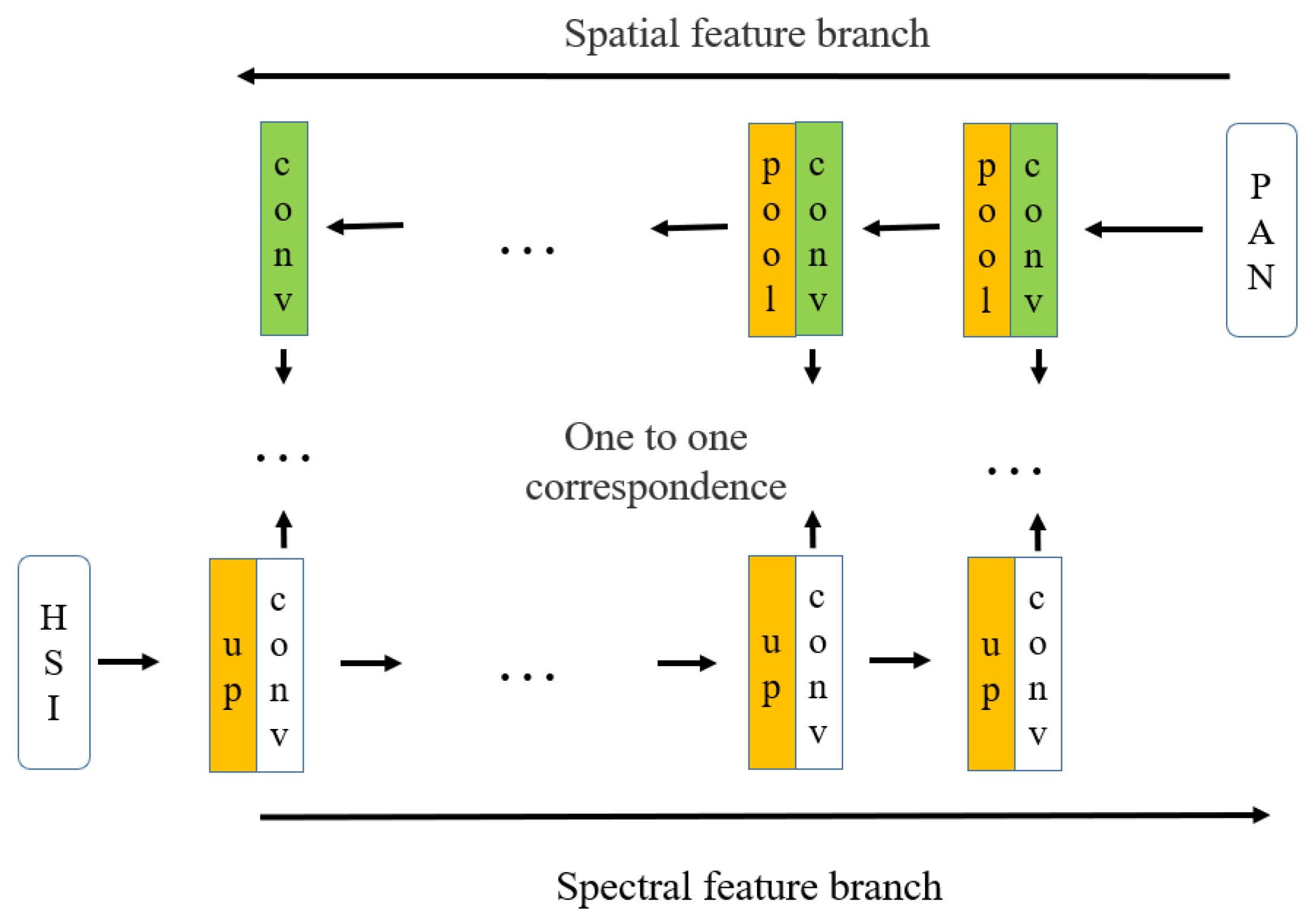
The schematic diagram of the establishment process of the spectral and spatial deep feature branches of hyperspectral and panchromatic images is shown in
Figure 1. Convolution operation is the core process in establishing spectral–spatial deep feature branches. The function of the convolution operation is to extract the features from the input data, and it contains multiple convolution kernels. Each element of the convolution kernel corresponds to a weight coefficient and a deviation quantity, which is like the neurons of a feedforward neural network. Each neuron in the convolutional layer relates to multiple neurons in the area close to the previous layer. The size of the area depends on the size of the convolutional nucleus, which is also called the receptive field and analogous to the receptive field of visual cortex cells. When the convolution kernel is working, it will sweep the input features regularly and sum the input features by matrix element multiplication in the receptive field and overlie the deviation. In
Figure 1, PAN represents the panchromatic image, HSI represents the hyperspectral image, conv represents the convolution operation, pool represents the pooling operation and up represents the up-sampling operation.
Hyperspectral images contain rich and detailed spectral information, while panchromatic images contain relatively rich spatial information. For hyperspectral and panchromatic images, the CNN is used to extract spectral and spatial deep features, respectively, and the two basic deep feature branches are established, which are spectral and spatial deep feature branches, respectively. In the branch of spatial deep feature, the panchromatic image is convoluted and pooled layer by layer to form spatial deep convolution features. Then spatial deep features are extracted layer by layer from panchromatic images and the establishment is completed for the spatial deep feature branch. The convolution operation on the branch of spatial deep feature is shown in Equation (1):
where
is the convolution operation,
is the deviation value,
and
represent the input and output of the
level convolution on the branch of spatial deep feature,
is the size of
,
is the pixel corresponding to the feature map,
is the number of channels of the feature map,
is the size of the convolution kernel,
is the convolution step size and
is the number of filling layers. The pooling operation on the branch of spatial deep feature is shown in Equation (2):
where
and
represent the input and output of the
level convolution on the branch of spatial deep feature, step length is
, pixel
has the same meaning as the convolution layer; when
,
pooling takes the mean value in the pooled area, which is called average-pooling; when
,
pooling takes the maximum value in the region, which is called max-pooling. The max-pooling method is adopted in this paper. At the same time, in the branch of spectral deep feature, the hyperspectral images are subjected to the up-sampling and convolution operation layer by layer to form the spectral deep convolution features. Then spectral deep features are extracted layer by layer from the hyperspectral remote sensing image and the establishment is completed for the spectral deep feature branch. The convolution operation on the spectral deep feature branch is shown in Equation (3):
where
and
represent the input and output of the
layer convolution on the spectral deep feature branch, the other parameters are similar to those of the convolution operation on the spatial feature branch.
Trilinear interpolation is used for the up-sampling procedure. Assuming that we want to know the value of the unknown function
at point
; meanwhile, supposing we know the values of the function
at four points
,
,
,
, then we implement linear interpolation in the
direction, as shown in Equation (4):
and then we implement linear interpolation in the
direction and obtain
, as shown in Equation (5):
There are the same number of levels in the two basic feature branches of the deep network, and the two basic branches of each layer correspond one-to-one. According to the same set of width ratio and spectral–spatial feature hierarchy between hyperspectral and panchromatic images, the level number of basic feature branches of two deep network is established. For panchromatic images, pooling down sampling between layers is used to obtain spatial convolution feature blocks of different sizes and dimensions for each layer. For hyperspectral images, the spectral convolution feature block with the same size as the corresponding spatial feature branch block is obtained by using up-sampling between layers. In this way, two basic spectral and spatial deep feature branches with corresponding feature blocks of the same size and dimension are established.
The schematic diagram of multi-scale residual enhancement of spatial deep features and residual enhancement for spectral deep features is shown in
Figure 2. In
Figure 2, the plus sign represents the residual block. This paper adopts residual network structure to adjust the spatial deep features in the spatial feature branch and then carries out multi-scale spatial information feature enhancement. Meanwhile, the proposed SSRN method also adopts residual network structure to enhance the spectral deep features in the spectral feature branch. Residual network allows original information transferring to the latter layers. For residual network, denoting desired underlying mapping function
, we let the stacked nonlinear layers fit another mapping as Equation (6):
where
is the residual part and
is the mapping part.
is residual variable and
is mapping variable. The original mapping is recast into Equation (7):
The formulation of
can be realized by feedforward neural networks with shortcut connections. The shortcut connections simply perform identity mapping, and their outputs are added to the outputs of the stacked layers. Identity shortcut connections add neither extra parameter nor computational complexity [
44]. For convolutional residual network with Equation (7), there is a convolutional operation in residual part
and an identity mapping with mapping part
. Convolutional residual network is adopted in the proposed SSRN method. Establishing the residuals of the network structure is based on the spatial feature branch at each level of convolution to join the original panchromatic image information to complete. Firstly, according to the size of the features of each convolution layer, pooling operation is adopted on panchromatic images. On the basis of the dimensions of each convolution layer, panchromatic images after pooling dimension are put on the stack, then the convolution results of each layer are added together to construct the spatial deep feature residual-enhanced network structure. Due to the different size and dimension of the convolution features in each layer, the sizes and dimensions of each convolution layer that joins the residuals of the network structure are not the same. Then the original panchromatic images in the spatial information in the form of multi-scale can join into the layers of convolution, which is formed of multi-scale spatial deep enhanced residual. In this way, the spatial features of panchromatic images are highlighted. In this paper, multi-scale residuals are added to the spatial deep feature branch of panchromatic images, which can enhance the spatial deep feature branch of panchromatic images to a certain extent. At the same time, residual network structure is also adopted in the spectral deep feature branch. In the spectral branch, residual network is only adopted in the final output convolution layer to enhance the spectral deep feature. In this procedure, trilinear interpolation up-sampling is adopted firstly to come up to the same spatial size as the final output convolution layer. Then, the up-sampling block is added to the final output convolution layer. The above representation is the procedure of spatial–spectral residual network operation. When the numbers of convolution layers on the spatial feature branch of panchromatic image and the spectral feature branch of hyperspectral image increase, the gradient will gradually disappear in the back propagation, and the underlying parameters cannot be effectively updated, resulting in the phenomenon of gradient disappearance. Or, when taking the derivative of the activation function, if the derivative is greater than 1, then when the number of layers increases, the gradient and novelty finally obtained will increase exponentially, resulting in the phenomenon of gradient explosion. The problem of gradient explosion or gradient vanishing will make the model training difficult to converge. By using the residual network, the gradient updated information can be transmitted from the upper level to the lower level during the back propagation, and the gradient explosion or gradient disappearance can be prevented. Therefore, adding the multi-scale residual enhancement network structure to the spatial deep feature branch and residual enhancement network structure to the spectral deep feature branch cannot only enhance the convolution feature on the spatial and spectral deep feature branch to a certain extent but also prevent the occurrence of gradient explosion or gradient disappearance. The pooling operation of spatial feature branch residual enhancement on panchromatic images is shown in Equation (8):
where
is the original panchromatic image,
is the multi-scale residuals on the convolution of the
layer that are enhanced by pooling results. Other parameters are like the pooling operation mentioned above. The result stacking operation after pooling is shown in Equation (9):
where
is the stack from the dimension
to
, and
is the dimension of the convolution of the corresponding
layer. Residual network is constituted with a series of residual block, which is constituted with mapping and residual parts. The operation of the residual enhancement network structure is shown in Equation (10):
where
is the result of the convolution at the
level on the spatial feature branch, and it is the mapping part for identity mapping in the residual block,
is the residual part in the residual block according to Equation (7),
is the result of enhanced residuals of the convolution of the
layer on the spatial feature branch. For convolutional residual network,
is represented with a convolution operation as Equation (11):
where
is the convolution weight of the
residual part,
is the biases of the
residual part. The other parameters are similar to those of the convolution operation on the spatial and spectral feature branch. Then,
is represented in Equation (12):
where
and
are the array formation of all of pixel
, then the array
is formulated with
here,
and
are the width and height of
. By substituting Equation (12) into Equation (10),
is obtained as Equation (13):
The trilinear interpolation of the original hyperspectral image for residual network on spectral feature branch is the same as Equations (4) and (5). After up-sampling, the residual network on spectral feature branch is shown in Equation (14):
where
is the original hyperspectral image after up-sampling,
is the final output convolution layer and it is the mapping part for identity mapping in the residual block. In addition,
is the residual part in the residual block according to Equation (7).
is the result of residual network on spectral deep feature branch. For convolutional residual network,
is represented with a convolution operation as Equation (15):
where
is the convolution weight of the residual part of the spectral residual network,
is the biases of the residual part of the spectral residual network. The other parameters are similar to those of the convolution operation on the spatial and spectral feature branch. Then,
is represented as Equation (16):
where
and
are the array formation of all of pixel
, then the array
is formulated with
here,
and
are the width and height of
. By substituting Equation (16) into Equation (14),
is obtained as Equation (17):
The schematic diagram of alignment for spectral and spatial deep features is shown in
Figure 3. The deep network established in this paper, after constructing the spectral and spatial deep feature branches, establishing multi-scale residual enhancement on the spatial feature branch and establishing residual enhancement on the spectral feature branch, builds the deep feature linkage of the spectral and the spatial feature branches. In addition, it adjusts the compatibility of the spatial and spectral deep features and makes the spatial and spectral deep features in the network more representational. Upon the completion of the spectral and spatial features in deep branches and multi-scale enhanced residual features in spatial and spectral feature branches, from low-level to high-level, spatial convolution correspond to the spectral convolution features from senior to junior. Both the existence of one-to-one correspondence with same sizes and dimensions are of the same convolution features. To make the spectral and spatial feature branches work together, the convolution feature blocks corresponding to each other with the same size and dimension are accumulated on the spectral feature branch, such that the corresponding convolution feature blocks in the spatial and spectral feature branches can be fused and interact. In this way, the obtained spectral and spatial accumulated features can have stronger feature characterization ability. After the establishment of spectral and spatial deep feature branches, the spatial deep feature multi-scale residual enhancement and spectral deep feature residual enhancement, and the spectral and spatial deep feature branches joint, the fusion image is finally output.
4. Discussion
This section refers to the discussion of the experimental results, evaluating the fusion performance of the proposed SSRN method. A series of performance indexes are adopted to precisely evaluate the spectral and spatial performance of the fusion results. Eight representative performance indexes are utilized in this paper. The performance indexes are Root Mean Squared Error (RMSE), Spectral Angle Mapper (SAM), Spatial Correlation Coefficient (SCC), spectral curve comparison, Peak-Signal-to-Noise Ratio (PSNR), Structural Similarity Index (SSIM), relative dimensionless global error in synthesis (ERGAS) and the Q metric [
24]. The RMSE, SAM, PSNR, SSIM, ERGAS and Q metric performance indexes have the characteristics of value. Meanwhile, the SCC and spectral curve comparison have the characteristics of value on each band. Then, RMSE, SAM, PSNR, SSIM, ERGAS and Q metric are shown in a value graph, and the SCC and spectral curve comparison is shown in a line graph to connect the value in each band. Here, spectral curve comparison is comparing spectral curves of a pixel in the result of the fusion method with the spectral curve of the corresponding pixel in the original hyperspectral image. In our experiments, we compare the spectral curve on the (360, 360) pixel in the fusion result of all the compared and proposed methods with the spectral curve on the (30, 30) pixel in the corresponding hyperspectral image for all three datasets. Among the performance indexes, SAM and spectral curve are spectral quality metrics, SCC and SSIM are spatial quality metrics and RMSE, PSNR, ERGAS and Q metric are comprehensive spatial–spectral quality metrics. We utilize the SAM, spectral curve comparison, RMSE, PSNR, ERGAS and Q metric to prove the spectral information enhancement on the high spatial-resolution image. In addition, we utilize the SCC, SSIM, RMSE, PSNR, ERGAS and Q metric to prove the spatial information enhancement on the hyperspectral image. It is important to emphasize that SAM, SCC, PSNR, SSIM and Q metric are better when they are larger, and RMSE, SAM and ERGAS are better when they are smaller. For SCC, the performance is better when most SCC values of bands are bigger than the other fusion methods. For spectral curve comparison, the performance is better when the spectral curve is near to the original spectral curve in the hyperspectral image.
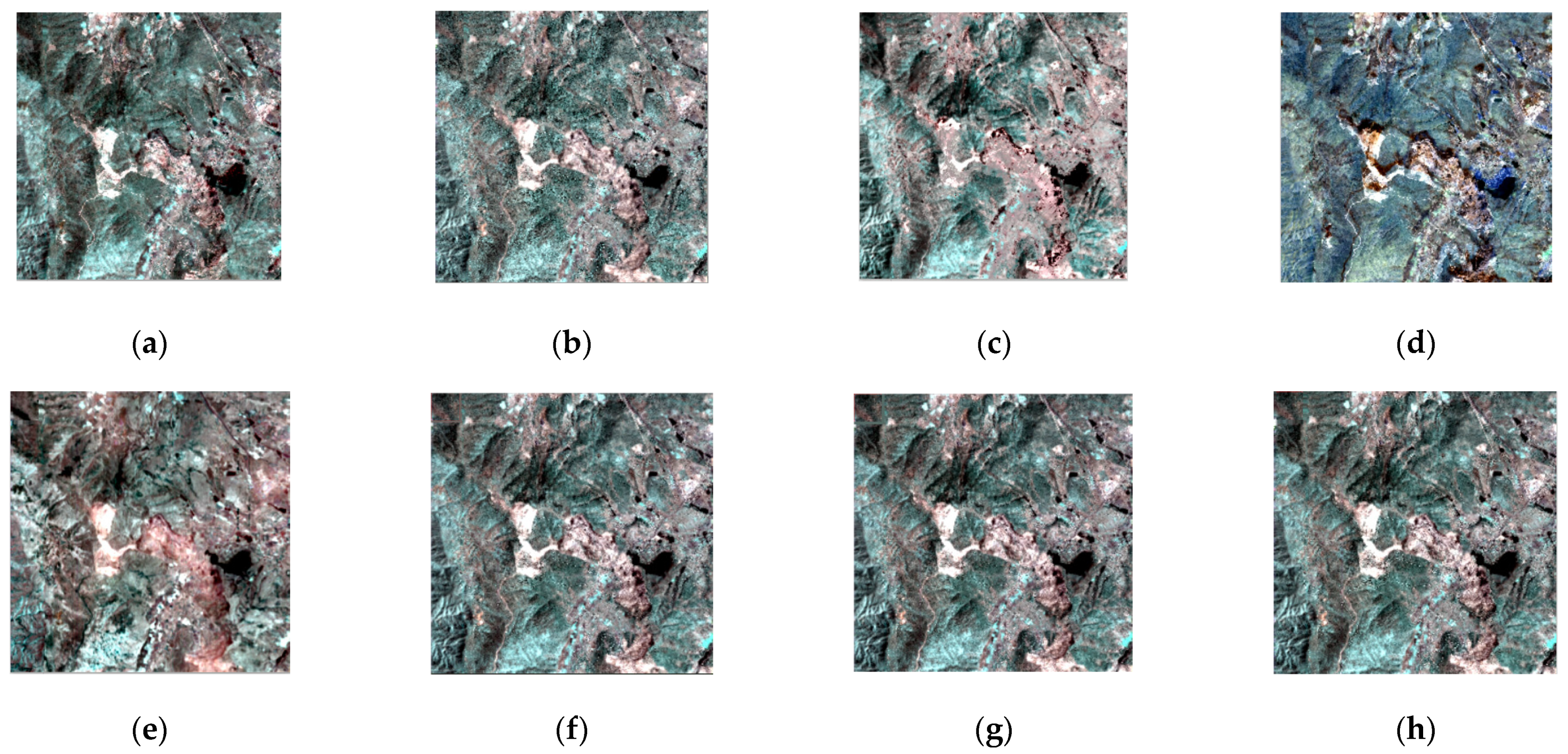
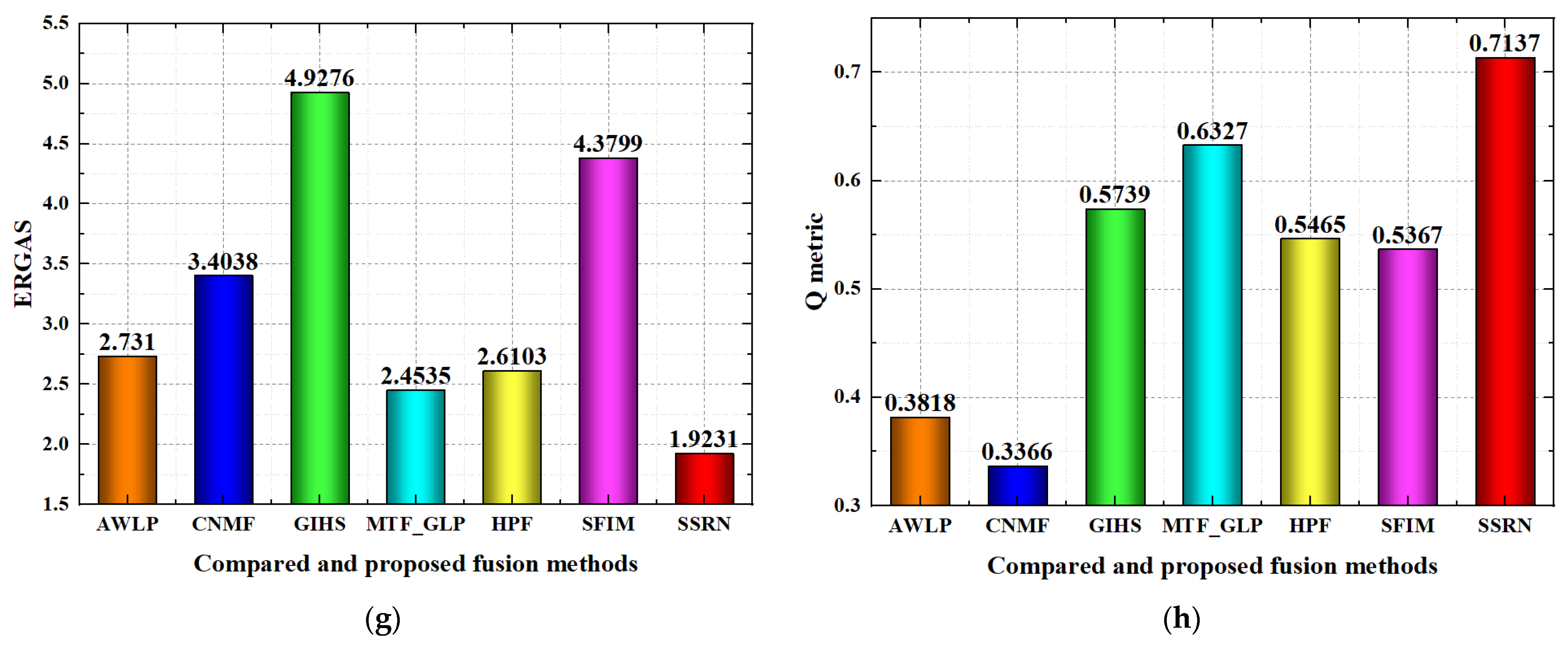
Quality evolution for the compared and proposed fusion methods on the Baiyangdian region dataset is shown in
Figure 10. For the RMSE index, the AWLP, MTF_GLP, HPF and the proposed SSRN methods achieve better performance than the CNMF, GIHS and SFIM methods to a great degree, while the proposed SSRN method achieves the best RMSE performance with RMSE lower than 100. For the SAM index, the AWLP, CNMF, MTF_GLP, HPF, SFIM and the proposed SSRN methods achieve better performance than the GIHS method to a great degree, while the SSRN method achieves the best performance. For the SCC index, GIHS and the proposed SSRN methods achieve better performance than the other compared methods, while the proposed SSRN method achieves the best SCC performance in most of the spectral bands. For the spectral curve comparison, the spectral curve of the proposed SSRN method is nearer than all of the compared fusion methods; then, the proposed SSRN method has better spectral curve comparison performance than the other compared fusion methods. For the PSNR index, AWLP, MTF_GLP, HFP and the proposed SSRN methods achieve better performance than the CNMF, GIHS and SFIM methods, and the proposed SSRN method achieves the best performance. For the SSIM index, GIHS, MTF_GLP, HPF and the proposed SSRN methods achieve better performance than the AWLP, CNMF and SFIM methods, and the proposed SSRN method achieves the best performance. For the ERGAS index, AWLP, MTF_GLP, HPF and the proposed SSRN methods achieve better performance than the CNMF, GIHS and SFIM methods, while the proposed SSRN method achieves the best performance. For the Q metric index, MTF_GLP and the proposed SSRN methods achieve better performance than the AWLP, CNMF, GIHS, HPF and SFIM methods, while the proposed SSRN method has the best performance.
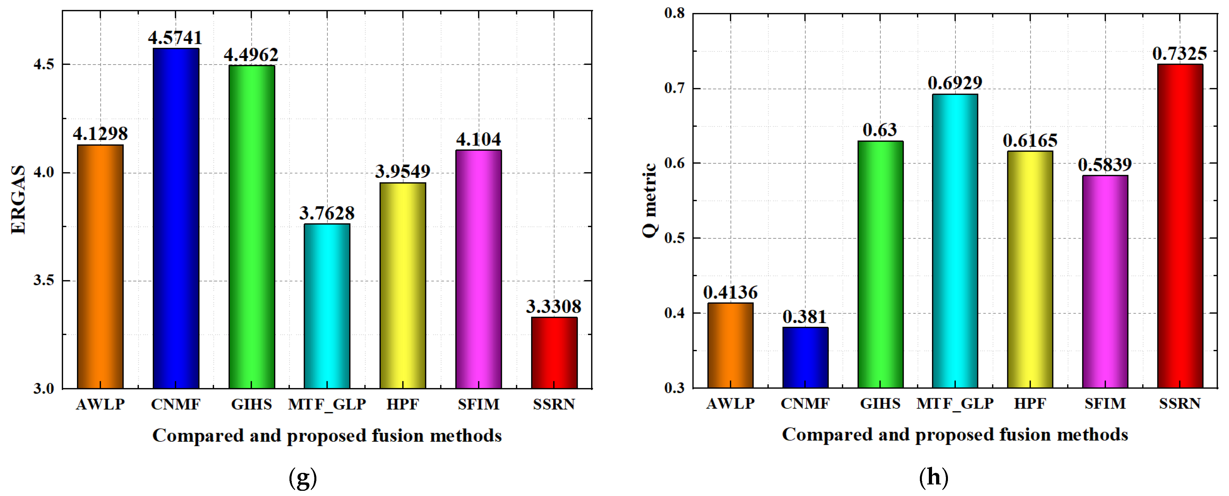
Quality evaluation for the compared and proposed methods on the Chaohu region dataset is shown in
Figure 11. For the RMSE index, the AWLP, MTF_GLP, HPF and the proposed SSRN methods achieve better performance than the CNMF, GIHS and SFIM methods to a great degree, while the proposed SSRN method achieves the best RMSE performance. For the SAM index, the AWLP, CNMF, MTF_GLP, HPF, SFIM and the proposed SSRN methods achieve better performance than the GIHS method to a great degree, while the SSRN method achieves the best performance. For the SCC index, the proposed SSRN method achieves better performance than all the compared methods in most of the spectral bands. For the spectral curve comparison, the spectral curve of the proposed SSRN method is nearer than all of the compared fusion methods; then, the proposed SSRN method has better spectral curve comparison performance than the other compared fusion methods. For the PSNR index, AWLP, MTF_GLP, HPF, SFIM and the proposed SSRN methods achieve better performance than CNMF and GIHS, and the proposed SSRN method achieves the best performance. For the SSIM index, GIHS, MTF_GLP, SFIM and the proposed SSRN methods achieve better performance than the AWLP, CNMF and HPF methods, while the proposed SSRN method achieves the best performance. For the ERGAS index, AWLP, CNMF, MTF_GLP, HPF and the proposed SSRN methods achieve better performance than the GIHS and SFIM methods, while the proposed SSRN method has the best performance. For the Q metric index, GIHS, MTF_GLP, HPF, SFIM and the proposed SSRN methods achieve better performance than the AWLP and CNMF methods, while the proposed SSRN method achieves the best performance.
Quality evaluation for the compared and proposed methods on the Dianchi region dataset is shown in
Figure 12. For the RMSE index, the AWLP, MTF_GLP, HPF, SFIM and the proposed SSRN methods achieve better performance than the CNMF and GIHS methods to a great degree, and the proposed SSRN method achieves the best RMSE performance. For the SAM index, the AWLP, CNMF, MTF_GLP, HPF, SFIM and the proposed SSRN methods achieve better performance than the GIHS method to a great degree, and the SSRN method achieves the best performance. For the SCC index, the proposed SSRN method achieves better performance than all the compared methods in most of the spectral bands. For the spectral curve comparison, AWLP, HPF, SFIM and the proposed SSRN methods achieve better performance than the CNMF, GIHS and MTF_GLP methods. The spectral curve of the proposed SSRN method is nearer than all of the compared fusion methods; then, the proposed SSRN method has better spectral curve comparison performance than the other compared fusion methods. For the PSNR index, AWLP, MTF_GLP, SFIM and the proposed SSRN methods achieve better performance than CNMF, GIHS and HPF methods, and the proposed SSRN method achieves the best performance. For the SSIM index, GIHS, MTF_GLP, HPF and the proposed SSRN methods achieve better performance than the AWLP, CNMF and SFIM methods, and the proposed SSRN method achieves the best performance. For the ERGAS index, MTF_GLP and the proposed SSRN methods achieve better performance than the AWLP, CNMF, GIHS, HPF, SFIM methods, while the proposed SSRN method achieves the best performance. For the Q metric index, GIHS, MTF_GLP, HPF, SFIM and the proposed SSRN methods achieve better performance than the AWLP and CNMF methods, while the proposed SSRN method achieves the best performance.
From discussing the performance indexes, some conclusions of the statistical reliability of the results can be concluded. With the spectral quality metrics of SAM, spectral curve comparison, RMSE, PSNR, ERGAS and Q metric indexes, the proposed SSRN method achieves the best performance; thus, the proposed SSRN method has strong reliability of spectral reconstruction ability. Meanwhile, with the spatial quality metrics of SCC, SSIM, RMSE, PSNR, ERGAS and Q metric indexes, the proposed SSRN method also achieves the best performance; thus, the proposed SSRN method also has strong reliability of spatial reconstruction ability. By the RMSE, ERGAS and Q metric indexes, the proposed SSRN method has strong reliability of holistic reconstruction similarity. By the SAM and spectral curve comparison indexes, the proposed SSRN method has strong reliability of spectral reconstruction similarity. By the SCC and SSIM indexes, the proposed SSRN method has strong reliability of spatial reconstruction similarity. By the PSNR index, the proposed SSRN method has reliability of more signal-to-noise-ratio reconstruction ability.
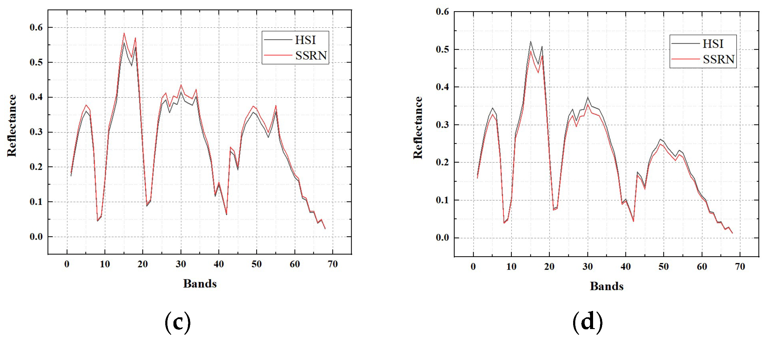
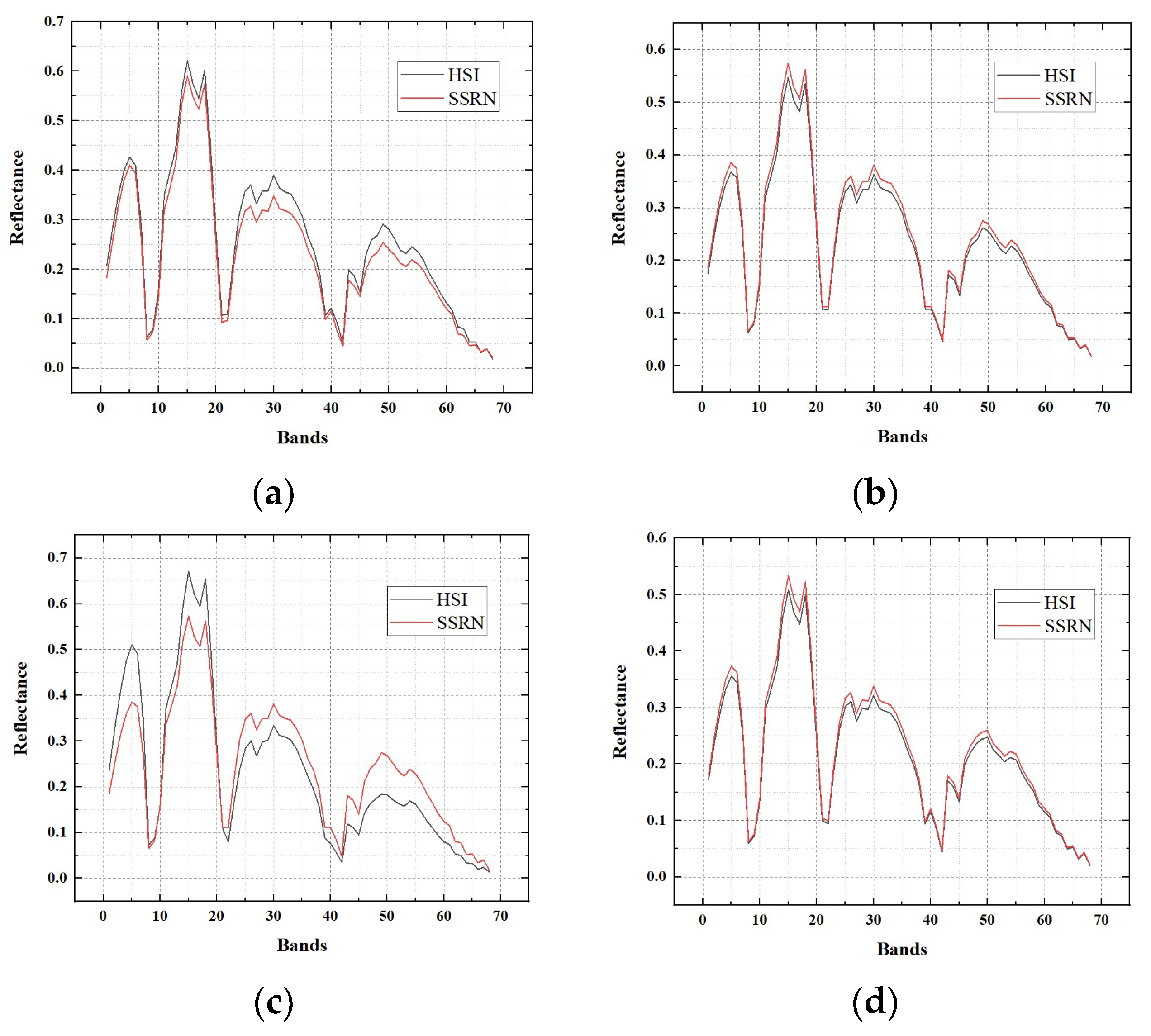
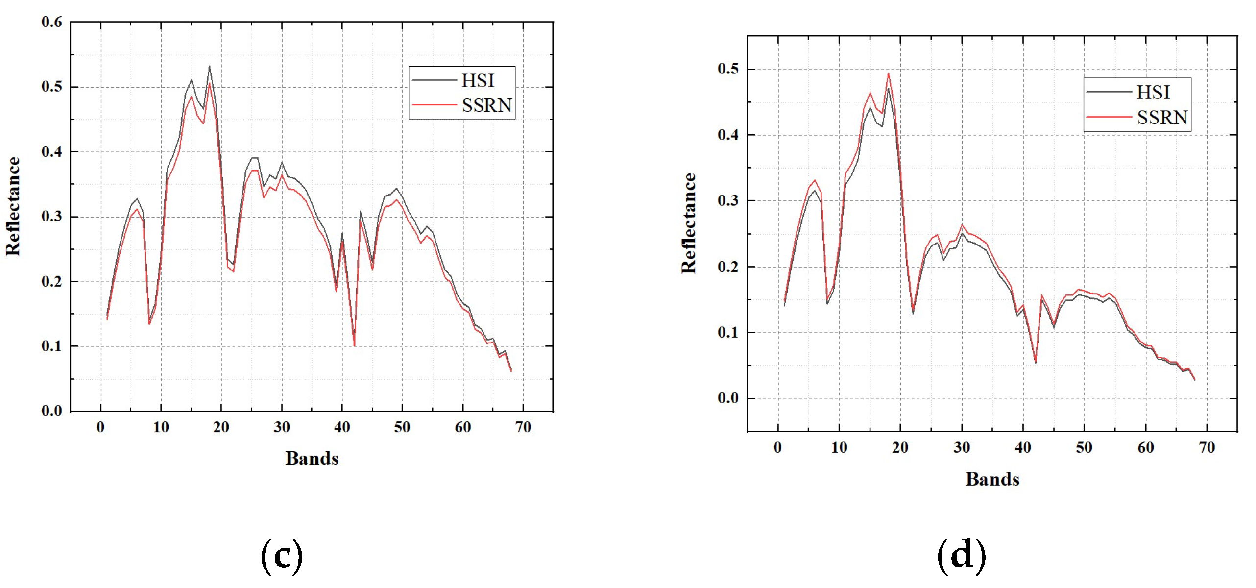
Here, we will provide the reflectance of the hyperspectral image and the SSRN fusion result on three experimental datasets. Reflectance of pixels (30, 30), (30, 270), (270, 30), (270, 270) in the hyperspectral image for each dataset is selected for the exhibition of reflectance. Accordingly, reflectance of pixels (360, 360), (360, 3240), (3240, 360), (3240, 3240) in the SSRN fusion result for each dataset is selected for the exhibition of reflectance.
Reflectance of four pixels in the Baiyangdian, Chaohu, Dianchi datasets are shown in
Figure 13,
Figure 14 and
Figure 15, respectively. From these figures, it can be seen that the fusion results of the proposed SSRN method have almost the same reflectance compared with the original hyperspectral images.
In terms of the discussion of the quality evaluation for the compared and proposed SSRN methods on the three datasets, it can be seen that the MTF_GLP method achieves the best evaluation performance in the compared fusion methods, while the GIHS method achieves worse fusion results than the other compared fusion methods. Meanwhile, the proposed SSRN method achieves better evaluation performance than all of the compared fusion methods.


