A GRU and AKF-Based Hybrid Algorithm for Improving INS/GNSS Navigation Accuracy during GNSS Outage

Abstract

The integrated navigation system consisting of an inertial navigation system (INS) and Global Navigation Satellite System (GNSS) provides continuous high-accuracy positioning whereas the navigation accuracy during a GNSS outage inevitably degrades owing to INS error divergence. To reduce such degradation, a gated recurrent unit (GRU) and adaptive Kalman filter (AKF)-based hybrid algorithm is proposed. The GRU network, which has advantages of high accuracy and efficiency, is constructed to predict the position variations during GNSS outage. Furthermore, this paper takes the GRU-predicted error accumulation into consideration, and introduces AKF as a supplementary methodology to improve the navigation performance. The proposed hybrid algorithm is trained and tested by practical road datasets and compared with four algorithms, including the standard KF, Multi-Layer Perceptron (MLP)-aided KF, Long Short Time Memory (LSTM) aided KF, and GRU-aided KF. Periods of 180 and 120 s GNSS outage are employed to test the performance of the proposed algorithm in different time scales. The comparison result between the standard KF and neural network-aided KF indicates that the neural network is an effective methodology for bridging GNSS outages. The performance comparison between three kinds of neural networks demonstrate that both recurrent neural networks surpass the MLP in prediction position variation, and the GRU transcends the LSTM in prediction accuracy and training efficiency. Furthermore, it is concluded that the adaptive estimation theory is an effective complement to neural network-aided navigation, as the GRU-aided AKF reduced the horizontal error of GRU-aided KF by 31.71% and 16.12% after 180 and 120 s of GNSS outage, respectively.

1. Introduction

INS and GNSS are two of the most widely used navigation techniques in both civilian and military fields. GNSS provides high accuracy position and velocity information with a relatively stable noise level in open-sky outdoor environments [1,2]. Nevertheless, it suffers from the shortcoming of signal vulnerability, which leads to accuracy degradation in complex urban environment, including overpasses, boulevards, and urban canyons, etc. On the other hand, INS is a self-contained navigation system that estimates the position, velocity, and attitude with a high update frequency. Although, INS suffers from a drawback in that its error accumulates over time [3]. Since INS and GNSS have complementary characteristics, they are combined as an INS/GNSS integrated navigation system which surpasses both stand-alone systems [4,5,6,7].

Although INS error could be estimated and compensated for by the KF-based INS/GNSS integration algorithm [8], low-cost INS error accumulates rapidly [9] during GNSS outage. Generally, there are, in general, two categories of techniques used to enhance low-cost INS /GNSS integrated navigation performance during GNSS outage. The first one is adopting auxiliary sensors, such as a camera [10,11,12,13], Lidar [14,15], magnetic sensor [16], or odometer [17,18], to collect various information to aid INS. The drawbacks of this kind of solution include increases in hardware cost, equipment volume, and power consumption. Another category of techniques is suppressing INS error accumulation by algorithm improvement without extra sensors. For instance, non-holonomic constraint (NHC) [17,19], assuming zero velocity at the land vehicle laterally and vertically, adopts pseudo velocity measurement to suppress INS velocity error divergence, and zero velocity update (ZUPT) [20] corrects INS error when the navigation system is stationary. Recently, the artificial intelligent (AI) algorithm has been employed in the navigation field due to its advantages of solving the non-linear problem, and AI-aided navigation systems have shown impressive performance. However, the AI algorithm also has the disadvantages of a long training time and the predicted value inevitably containing error. The former disadvantage could be partly solved by simplifying the neural network structure while the latter one could be suppressed using the adaptive algorithm. Thus, this paper constructed a simple and effective GRU network to aid INS during GNSS outage, and adopts the AKF algorithm to estimate pseudo position measurement noise, thus optimizing the integrated navigation accuracy.

The novelties of this paper are summarized as follows: (1)A GRU-based pseudo GNSS position variation prediction neural network is proposed in this work. The proposed network is verified to have the advantages of a high prediction accuracy and high training efficiency. (2) Meanwhile, different from existing related AI methodology, this work takes the AI prediction error into consideration. An adaptive filtering strategy is adopted as the supplement of the GRU network, and the Sage-Husa AKF is introduced to estimate the state vector and pseudo GNSS position noise simultaneously. The rationale behind this methodology is that assigning proper weight to the GRU-predicted information during the INS and pseudo GNSS data fusion process improves the navigation performance.

The structure of the remaining part is organized as follow. The rationale of the GRU and AKF hybrid algorithm is presented in Section 2. Then, the detailed GRU network implement method is described in Section 3, followed by the test and result analysis in Section 4. Finally, the discussion and conclusions are put forward in Section 5 and Section 6, respectively.

2. Rationale of the Proposed Algorithm

2.1. AI Module Input and Output Parameters

It is crucial to select proper input and output parameters for the AI module, since these parameters directly determine the navigation accuracy and training efficiency. All existing AI models applied in bridging GNSS outage can be divided into three categories. The first kind is the O_INS-δP_{GNSS, INS} model [21,22,23,24,25], which predicts δP_{GNSS, INS} standing for the position error between GNSS measurement and INS estimation with the input parameters O_INS (including the position, velocity, attitude estimated by INS, and angular velocity, specific force measured by the inertial measurement unit). Another category is O_INS-X model [26], which estimates the state vector X of the integrated navigation system directly. The third type of model O_INS-ΔP_GNSS [27,28,29], which calculates the GNSS position variation ΔP_GNSS, is adopted in this paper. The GNSS position variation error is expressed in Equation (1), where $\Delta {\widehat{\mathrm{P}}}_{\mathrm{GNSS}}{(\mathrm{t}}_{\mathrm{k}})$ is the estimated position variance between epochs ${\mathrm{t}}_{\mathrm{k}}$ and ${\mathrm{t}}_{\mathrm{k}-1}$, and ${\widehat{\mathrm{P}}}_{\mathrm{GNSS}}{(\mathrm{t}}_{\mathrm{k}})$ and ${\widehat{\mathrm{P}}}_{\mathrm{GNSS}}{(\mathrm{t}}_{\mathrm{k}-1})$ represent the estimated position at ${\mathrm{t}}_{\mathrm{k}}$ and ${\mathrm{t}}_{\mathrm{k}-1}$, respectively. The estimated position ${\widehat{\mathrm{P}}}_{\mathrm{GNSS}}{(\mathrm{t}}_{\mathrm{k}})$ consists of the truth value ${\mathrm{P}}_{\mathrm{GNSS}}\left({\mathrm{t}}_{\mathrm{k}}\right)$ and the error term ${\mathsf{\delta }\mathrm{P}}_{\mathrm{GNSS}}\left({\mathrm{t}}_{\mathrm{k}}\right)$.${\widehat{\mathrm{P}}}_{\mathrm{GNSS}}{(\mathrm{t}}_{\mathrm{k}-1})$ similarly consists of the truth value ${\mathrm{P}}_{\mathrm{GNSS}}\left({\mathrm{t}}_{\mathrm{k}-1}\right)$ and the error term ${\mathsf{\delta }\mathrm{P}}_{\mathrm{GNSS}}\left({\mathrm{t}}_{\mathrm{k}-1}\right)$. It can be deduced from the formula that differential arithmetic between adjacent epochs could remove the GNSS measurement noise, which has time correlativity. In other words, the O_INS-ΔP_GNSS model has lower prediction error than the former two models:

$$\begin{array}{l}\Delta {\widehat{\mathrm{P}}}_{\mathrm{GNSS}}({\mathrm{t}}_{\mathrm{k}})={\widehat{\mathrm{P}}}_{\mathrm{GNSS}}{(\mathrm{t}}_{\mathrm{k}})-{\widehat{\mathrm{P}}}_{\mathrm{GNSS}}({\mathrm{t}}_{\mathrm{k}-1})=({\mathrm{P}}_{\mathrm{GNSS}}\left({\mathrm{t}}_{\mathrm{k}}\right)+{\mathsf{\delta }\mathrm{P}}_{\mathrm{GNSS}}\left({\mathrm{t}}_{\mathrm{k}}\right))\\ -\left({\mathrm{P}}_{\mathrm{GNSS}}\left({\mathrm{t}}_{\mathrm{k}-1}\right)+{\mathsf{\delta }\mathrm{P}}_{\mathrm{GNSS}}\left({\mathrm{t}}_{\mathrm{k}-1}\right)\right)=\Delta {\mathrm{P}}_{\mathrm{GNSS}}\left({\mathrm{t}}_{\mathrm{k}}\right)-\left({\mathsf{\delta }\mathrm{P}}_{\mathrm{GNSS}}\left({\mathrm{t}}_{\mathrm{k}}\right)-{\mathsf{\delta }\mathrm{P}}_{\mathrm{GNSS}}\left({\mathrm{t}}_{\mathrm{k}-1}\right)\right)\end{array}$$

(1)

The position variation $\Delta {\mathrm{P}}_{\mathrm{GNSS}}{(\mathrm{t}}_{\mathrm{k}})$can also be expressed as the difference in the INS derived position between adjacent epochs as shown in Equation (2):

$${\mathsf{\Delta }\mathrm{P}}_{\mathrm{GNSS}}=\iint \left({\mathrm{C}}_{\mathrm{b}}^{\mathrm{n}}{\mathrm{f}}_{\mathrm{ib}}^{\mathrm{b}}\left(\mathrm{t}\right)-\left({2\mathsf{\omega }}_{\mathrm{ie}}^{\mathrm{n}}\left(\mathrm{t}\right)+{\mathsf{\omega }}_{\mathrm{en}}^{\mathrm{n}}\left(\mathrm{t}\right)\right)\text{×}{\mathrm{V}}^{\mathrm{n}}\left(\mathrm{t}\right)+{\mathrm{G}}^{\mathrm{n}}\right)\mathrm{dtdt}$$

(2)

where b, i, e, and n stand for the body frame (b-frame), inertial frame (i-frame), earth frame (e-frame), and navigation frame (n-frame), respectively. ${\mathrm{C}}_{\mathrm{b}}^{\mathrm{n}}$ is the directional cosine matrix from the n-frame to b-frame, ${\mathrm{f}}_{\mathrm{ib}}^{\mathrm{b}}$ is the specific force acquired by the inertial measurement unit (IMU), ${\mathsf{\omega }}_{\mathrm{ie}}^{\mathrm{n}}$ is the angular rate of the e-frame relative to the i-frame, ${\mathsf{\omega }}_{\mathrm{en}}^{\mathrm{n}}$ is the angular rate of the n-frame relative to the e-frame, ${\mathrm{V}}^{\mathrm{n}}$ is the INS-derived velocity, and ${\mathrm{G}}^{\mathrm{n}}$ is the gravity vector. Since ${\mathsf{\omega }}_{\mathrm{ie}}^{\mathrm{n}}$,${\mathsf{\omega }}_{\mathrm{en}}^{\mathrm{n}}$, and ${\mathrm{G}}^{\mathrm{n}}$ are related to the longitude and latitude, which vary slowly in land vehicles, these three parameters can be neglected to improve the training efficiency. The input parameters of the AI model are the IMU data, including ${\mathrm{f}}_{\mathrm{ib}}^{\mathrm{b}}$ and ${\mathsf{\omega }}_{\mathrm{ib}}^{\mathrm{b}}$ and the INS-estimated velocity (${\mathrm{V}}^{\mathrm{n}}$) and attitude (${\mathrm{A}}_{\mathrm{INS}})$.

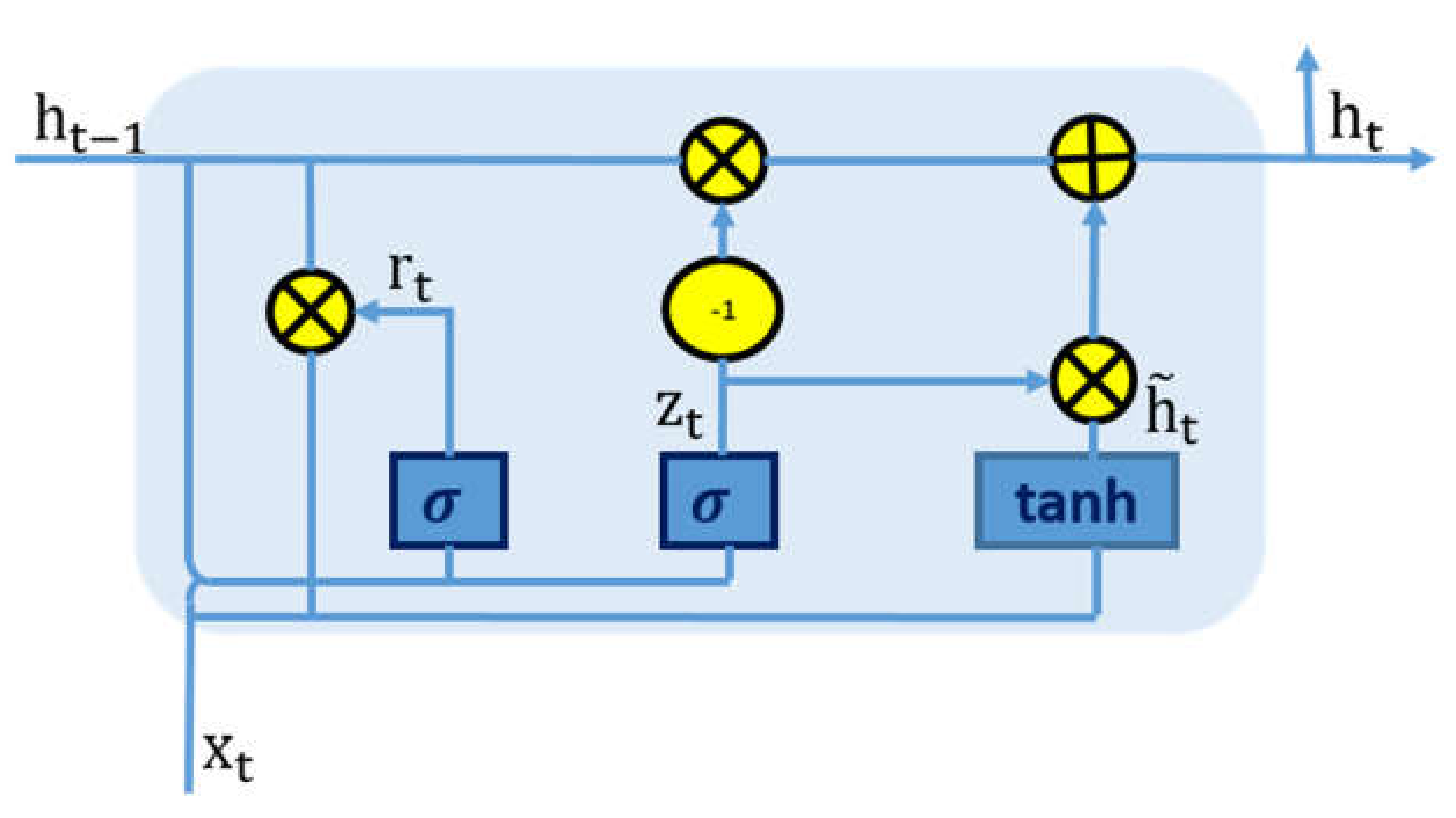
2.2. Neural Network Model: GRU

Various neural network models are adopted in AI-aided integrated navigation. Assad adopted the radial basis function neural network (RBF) to improve the attitude estimation accuracy in GPS-denied environments [30]. Yao estimated the pseudo GPS position with the MLP network when GPS signal was unavailable [28]. However, these methods employ a static neural network, which only deals with current data but neglects the information of historical data. Neglecting the historical data may result in a low prediction accuracy. Thus, the recurrent neural network that is widely used in time series signals processing is a better choice for integrated navigation. Fang suggested a method for bridging GNSS outage that used a kind of recurrent neural network called the LSTM, and obtained a satisfying effect [29]. The GRU, which is also a recurrent neural network, with the same estimation accuracy and higher training efficiency compared with LSTM [31], is adopted in this paper. As shown in Figure 1, the GRU unit consists of an update gate and a reset gate. The output of the update gate (z_t) controls the extent of the impact on the current state forced by previous states; that is, the smaller z_t is, the less previous information is retained. The function of the reset gate(r_t) is to determine the forgetfulness degree of the hidden state information $\widetilde{{\mathrm{h}}_{\mathrm{t}}}$; that is, the smaller the value is, the more past state information is discarded.

The GRU forward propagation formula is shown in Equation (3):

$$\begin{gathered} {\mathrm{r}}_{\mathrm{t}}={\mathsf{\sigma }(\mathrm{W}}_{\mathrm{xr}}{\mathrm{x}}_{\mathrm{t}}{+\mathrm{W}}_{\mathrm{hr}}{\mathrm{h}}_{\mathrm{t}-1}+{\mathrm{b}}_{\mathrm{r}}) \\ {\mathrm{z}}_{\mathrm{t}}={\mathsf{\sigma }(\mathrm{W}}_{\mathrm{xz}}{\mathrm{x}}_{\mathrm{t}}+{\mathrm{W}}_{\mathrm{hz}}{\mathrm{h}}_{\mathrm{t}-1}+{\mathrm{b}}_{\mathrm{z}}) \\ {\tilde{\mathrm{h}}}_{\mathrm{t}}{\mathrm{h}}_{\mathrm{t}}={\mathrm{z}}_{\mathrm{t}}\odot {\mathrm{h}}_{\mathrm{t}-1}+{(1-\mathrm{z}}_{\mathrm{t}})\odot {\tilde{\mathrm{h}}}_{\mathrm{t}}=\tanh ({\mathrm{W}}_{\mathrm{xh}}{\mathrm{x}}_{\mathrm{t}}+{\mathrm{W}}_{\mathrm{hh}}{(\mathrm{r}}_{\mathrm{t}}\odot {\mathrm{h}}_{\mathrm{t}-1})+{\mathrm{b}}_{\mathrm{h}}) \\ {\mathrm{h}}_{\mathrm{t}}={\mathrm{z}}_{\mathrm{t}}\odot {\mathrm{h}}_{\mathrm{t}-1}+{(1-\mathrm{z}}_{\mathrm{t}})\odot {\tilde{\mathrm{h}}}_{\mathrm{t}} \end{gathered}$$

(3)

where, $\mathrm{W}$ represents the weight matrix between different structures; subscripts x, r, h, and z denote the input, reset gate, hidden state, and update gate; and ${\mathrm{b}}_{\mathrm{r}}$, ${\mathrm{b}}_{\mathrm{z}}$, and ${\mathrm{b}}_{\mathrm{h}}$are the offset vectors of the corresponding structure.

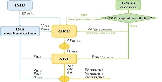
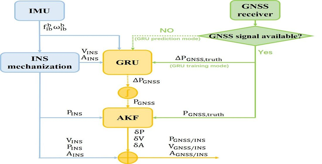
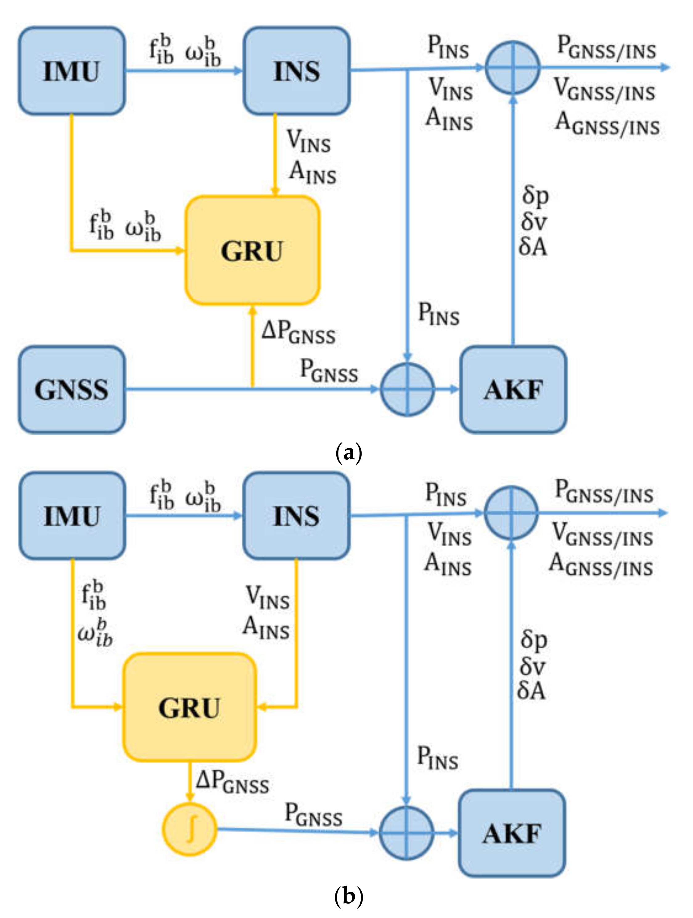
2.3. Proposed GRU-aided AKF Algorithm

The proposed INS/GNSS integrated navigation algorithm employs an AKF-based loosely coupled integration strategy with a GRU module, which works in training mode when GNSS signal is available and prediction mode during a GNSS outage.

According to the above analysis, the proposed scheme consisting of the training mode and predicting mode is illustrated in Figure 2. As shown in Figure 2a, the GRU module operates in training mode when GNSS signal is available. With the input parameters of ${\mathrm{f}}_{\mathrm{ib}}^{\mathrm{b}}$, ${\mathsf{\omega }}_{\mathrm{ib}}^{\mathrm{b}}$, ${\mathrm{V}}^{\mathrm{n}}$, and ${\mathrm{A}}_{\mathrm{INS}}$, the GRU module outputs the predicted position variance ΔP_GNSS, which is compared with the high precision ΔP_true representing the position variation derived from the real GNSS signal. The GRU module adjusts the internal weight continuously until the loss function drops below the threshold. Meanwhile, the KF module works as a traditional loosely coupled integrated navigation system, providing high accuracy position, velocity, attitude, and IMU error information in real time. When GNSS signal is unavailable, the GRU module operates in the predicting mode shown in Figure 2b. The GRU module predicts the position variation ΔP_GNSS, which is integrated as a pseudo GNSS position measurement. Because ΔP_GNSS inevitably includes error, the pseudo position measurement also includes error, which increases during the ΔP_GNSS integral process. However, all existing literature [23,24,25] that adopted the O_INS-ΔP_GNSS model did not take this phenomenon into consideration.

In this paper, the 15-dimentional state vector X is defined as X = [δr, δv, φ, b_g, b_a] ^T, where δr and δv are the 3-dimensional INS position error and velocity error in the n-frame, φ stands for the misalignment angles, and b_g and b_a are the gyroscope and accelerometer bias in the x axis, y axis, and z axis. The three-dimensional measurement vector Z is defined as the difference between the INS-estimated position and the GRU-estimated position. The discrete-time Kalman state function and measurement function are defined as Equation (4):

$$\begin{array}{l}{\mathrm{X}}_{\mathrm{k}}{=\mathsf{\Phi }}_{\mathrm{k}|\mathrm{k}-1}{\mathrm{X}}_{\mathrm{k}-1}{+\mathsf{\Gamma }}_{\mathrm{k}-1}{\mathsf{\omega }}_{\mathrm{k}-1}\\ {\mathrm{Z}}_{\mathrm{k}}{=\mathrm{H}}_{\mathrm{k}}{\mathrm{X}}_{\mathrm{k}}{+\mathrm{V}}_{\mathrm{k}}\end{array}$$

(4)

where X_k is the state vector at time k, Φ_k|k−1 is the one-step state transition matrix from time k − 1 to k, Γ_k−1 is the system noise-input mapping matrix, ω_k−1 is the system noise vector presenting a zero mean Gauss distribution with variance Q_k−1, Z is the measurement vector, H_k represents the measurement matrix, and V_k is the measurement noise vector subjected to a zero mean Gauss distribution with variance R_k−1. Theoretically, KF could acquire an optimal estimation when noise statistical parameters, such as Q_k−1 and R_k−1, are precisely known [32]. However, the ΔP_GNSS predicted by the GRU module inevitably contains error, which is accumulated when ΔP_GNSS is integral to P_GNSS. All the existing literatures utilizing the O_INS-ΔP_GNSS model [27,28,29] did not take this phenomenon into consideration.

Standard KF includes the time update and measurement update process. The time update process is formulized as Equation (5):

$$\begin{array}{l}{\widehat{\mathrm{X}}}_{\mathrm{k}|\mathrm{k}-1}={\mathsf{\Phi }}_{\mathrm{k}|\mathrm{k}-1}{\widehat{\mathrm{X}}}_{\mathrm{k}-1}\\ {\mathrm{P}}_{\mathrm{k}|\mathrm{k}-1}={\mathsf{\Phi }}_{\mathrm{k}|\mathrm{k}-1}{\mathrm{P}}_{\mathrm{k}-1}{\mathsf{\Phi }}_{\mathrm{k}|\mathrm{k}-1}^{\mathrm{T}}+{\mathsf{\Gamma }}_{\mathrm{k}-1}{\mathrm{Q}}_{\mathrm{k}-1}{\mathsf{\Gamma }}_{\mathrm{k}-1}^{\mathrm{T}}\end{array}$$

(5)

where ${\widehat{\mathrm{X}}}_{\mathrm{k}|\mathrm{k}-1}$ is the prediction of the state vector at time k, ${\widehat{\mathrm{X}}}_{\mathrm{k}-1}$ is the optimal estimation at time k − 1, ${\mathrm{P}}_{\mathrm{k}|\mathrm{k}-1}$ is the prediction covariance matrix at time k, and ${\mathrm{P}}_{\mathrm{k}-1}$ is the optimal covariance matrix estimation at k − 1.

The KF measurement update process is illustrated in Equation (6):

$$\begin{array}{l}{\mathrm{K}}_{\mathrm{k}}={\mathrm{P}}_{\mathrm{k}|\mathrm{k}-1}{\mathrm{H}}_{\mathrm{k}}^{\mathrm{T}}{\left({\mathrm{H}}_{\mathrm{k}}{\mathrm{P}}_{\mathrm{k}|\mathrm{k}-1}{\mathrm{H}}_{\mathrm{k}}^{\mathrm{T}}{+\mathrm{R}}_{\mathrm{k}}\right)}^{-1}\\ {\widehat{\mathrm{X}}}_{\mathrm{k}}={\widehat{\mathrm{X}}}_{\mathrm{k}|\mathrm{k}-1}+{\mathrm{K}}_{\mathrm{k}}{(\mathrm{Z}}_{\mathrm{k}}-{\mathrm{H}}_{\mathrm{k}}{\widehat{\mathrm{X}}}_{\mathrm{k}|\mathrm{k}-1})\\ {\mathrm{P}}_{\mathrm{k}}=({\mathrm{I}-\mathrm{K}}_{\mathrm{k}}{\mathrm{H}}_{\mathrm{k}}){\mathrm{P}}_{\mathrm{k}|\mathrm{k}-1}{\left({\mathrm{I}-\mathrm{K}}_{\mathrm{k}}{\mathrm{H}}_{\mathrm{k}}\right)}^{\mathrm{T}}+{\mathrm{K}}_{\mathrm{k}}{\mathrm{R}}_{\mathrm{k}}{\mathrm{R}}_{\mathrm{k}}{}^{\mathrm{T}}\end{array}$$

(6)

where ${\mathrm{K}}_{\mathrm{k}}$ is the KF gain, and ${\widehat{\mathrm{X}}}_{\mathrm{k}}$ and ${\mathrm{P}}_{\mathrm{k}}$ are the optimal estimated state and its covariance matrix, respectively.

In order to furtherly improve the accuracy, the pseudo noise increase (namely the time-varying R) of the O_INS-ΔP_GNSS model should be taken into consideration. The Sage-Husa filter, which was proposed with a standard KF framework with the capability of estimating the system state and noise parameters simultaneously, is a solution for the increasing pseudo measurement noise. Its essence is matching the theoretical covariance of the innovation or residual sequence with its practical equivalent [33]. The former methodology is also known as the IAE (innovation-based adaptive estimation) filter and the latter one as the RAE (residual-based adaptive estimation) filter. The RAE can only estimate noise covariance with residuals prior to the current epoch, and once the current epoch measurement precision is inconsistent with the historical precision, it is hard for this methodology to guarantee estimation reliability [34]. Therefore, the IAE filter is adopted in this paper.

The innovation is defined as Equation (7) shows:

$$\begin{array}{l}{\tilde{\mathrm{Z}}}_{\mathrm{k}|\mathrm{k}-1}={\mathrm{Z}}_{\mathrm{k}}{-\widehat{\mathrm{Z}}}_{\mathrm{k}|\mathrm{k}-1}\\ =\left({\mathrm{H}}_{\mathrm{k}}{\mathrm{X}}_{\mathrm{k}}{+\mathrm{V}}_{\mathrm{k}}\right){-\mathrm{H}}_{\mathrm{k}}{\widehat{\mathrm{X}}}_{\mathrm{k}|\mathrm{k}-1}\\ ={\mathrm{H}}_{\mathrm{k}}{\tilde{\mathrm{X}}}_{\mathrm{k}|\mathrm{k}-1}{+\mathrm{V}}_{\mathrm{k}}\end{array}$$

(7)

The state prediction error ${\tilde{\mathrm{X}}}_{\mathrm{k}|\mathrm{k}-1}$is unbiased as the initial value is unbiased, and the mean of the measured noise V_k is assumed to be zero. It can be concluded that the innovation is zero mean. Since ${\tilde{\mathrm{X}}}_{\mathrm{k}|\mathrm{k}-1}$ and V_k are unrelated, the variance of ${\tilde{\mathrm{Z}}}_{\mathrm{k}|\mathrm{k}-1}$ can be expressed as Equation (8):

$$\mathrm{E}\left[{\tilde{\mathrm{Z}}}_{\mathrm{k}/\mathrm{k}-1}{\tilde{\mathrm{Z}}}_{\mathrm{k}/\mathrm{k}-1}^{\mathrm{T}}\right]{=\mathrm{H}}_{\mathrm{k}}{\mathrm{P}}_{\mathrm{k}/\mathrm{k}-1}{\mathrm{H}}_{\mathrm{k}}^{\mathrm{T}}{+\mathrm{R}}_{\mathrm{k}}$$

(8)

The measurement noise matrix R_k is presented as:

$${\mathrm{R}}_{\mathrm{k}}=\mathrm{E}\left[{\tilde{\mathrm{Z}}}_{\mathrm{k}/\mathrm{k}-1}{\tilde{\mathrm{Z}}}_{\mathrm{k}/\mathrm{k}-1}^{\mathrm{T}}\right]-{\mathrm{H}}_{\mathrm{k}}{\mathrm{P}}_{\mathrm{k}/\mathrm{k}-1}{\mathrm{H}}_{\mathrm{k}}^{\mathrm{T}}$$

(9)

In theory, $\mathrm{E}\left[{\tilde{\mathrm{Z}}}_{\mathrm{k}/\mathrm{k}-1}{\tilde{\mathrm{Z}}}_{\mathrm{k}/\mathrm{k}-1}^{\mathrm{T}}\right]$ can be replaced by the innovation average value over time, and the ${\mathrm{R}}_{\mathrm{k}}$ equally weighted recursive estimation equation can be constructed as Equation (10):

$$\begin{array}{l}{\widehat{\mathrm{R}}}_{\mathrm{k}}=\frac{1}{\mathrm{k}}{\displaystyle {\displaystyle \sum }_{\mathrm{i}=1}^{\mathrm{k}}}\left({\tilde{\mathrm{Z}}}_{\mathrm{i}|\mathrm{i}-1}{\tilde{\mathrm{Z}}}_{\mathrm{i}|\mathrm{i}-1}^{\mathrm{T}}{-\mathrm{H}}_{\mathrm{i}}{\mathrm{P}}_{\mathrm{i}|\mathrm{i}-1}{\mathrm{H}}_{\mathrm{i}}^{\mathrm{T}}\right)\\ =\frac{1}{\mathrm{k}}\left[\left(\mathrm{k}-1\right){\widehat{\mathrm{R}}}_{\mathrm{k}-1}+\left({\tilde{\mathrm{Z}}}_{\mathrm{k}|\mathrm{k}-1}{\tilde{\mathrm{Z}}}_{\mathrm{k}|\mathrm{k}-1}^{\mathrm{T}}{-\mathrm{H}}_{\mathrm{k}}{\mathrm{P}}_{\mathrm{k}|\mathrm{k}-1}{\mathrm{H}}_{\mathrm{k}}^{\mathrm{T}}\right)\right]\\ =\left(1-\frac{1}{\mathrm{k}}\right){\widehat{\mathrm{R}}}_{\mathrm{k}-1}+\frac{1}{\mathrm{k}}\left({\tilde{\mathrm{Z}}}_{\mathrm{k}|\mathrm{k}-1}{\tilde{\mathrm{Z}}}_{\mathrm{k}|\mathrm{k}-1}^{\mathrm{T}}{-\mathrm{H}}_{\mathrm{k}}{\mathrm{P}}_{\mathrm{k}|\mathrm{k}-1}{\mathrm{H}}_{\mathrm{k}}^{\mathrm{T}}\right)\end{array}$$

(10)

The Sage-Husa AKF is fully constructed while the ${\widehat{\mathrm{R}}}_{\mathrm{k}}$is substituted into Equation (6), and the filter can estimate the noise matrix in time and adjust the KF gain.

3. Implementation of the Proposed Algorithm

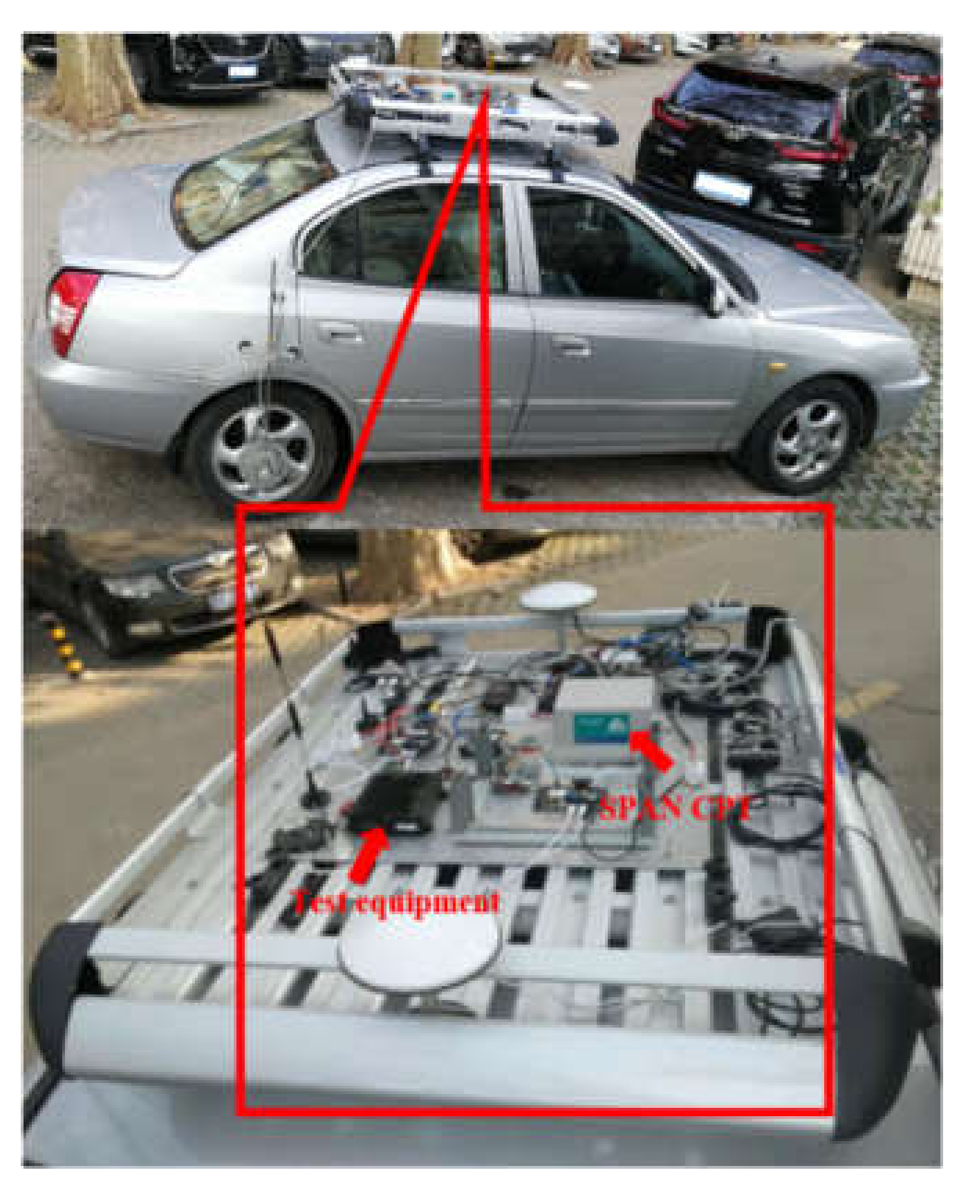
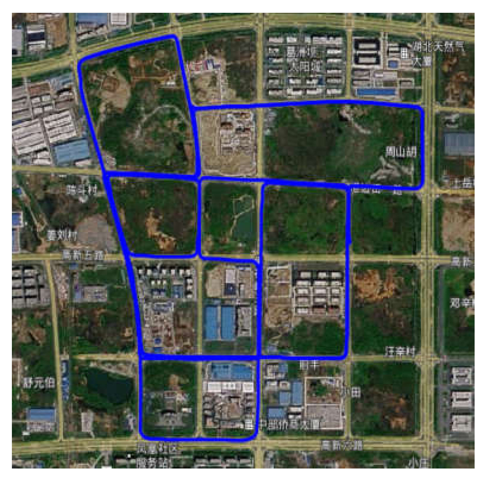
3.1. Training and Testing Dataset Description

In order to train and verify the performance of the proposed algorithm, a dataset was acquired with equipment mounted on a land vehicle shown in Figure 3. The data collection equipment consisted of micro-electromechanical systems (MEMSs) IMU whose crucial specifications are summarized in

Table 1. Hardware specifications.

Performance Parameter
Gyroscope bias stability	8°/h
Gyroscope angle random walk	0.12°/sqrt(h)
Accelerometer bias stability	0.2 mg
Accelerometer velocity random walk	0.09m/s/sqrt(h)

and a single-frequency GNSS receiver chip. Meanwhile, a set of reference data was gathered with NovAtel SPAN CPT.experimental platform.

The dataset was collected in Wuhan City, Hubei Province, China, and the dataset collection trajectory is shown in Figure 4. The total length of the dataset was 5200 s (GPS time: 198,900–204,100). Among them, data from GPS time 198,900 to 201,900 s were utilized as the GRU network training dataset, and data from GPS time 201,900 to 204,100 s were used as the testing dataset.

3.2. Training Process

The GRU module was trained with 12 input parameters, including the 3-axis gyroscope data, 3-axis accelerometer data, and 3-axis velocity and attitude data. Meanwhile, the GNSS position variation ΔP_GNSS was taken as the training label. To balance the training efficiency and predicting accuracy, the GRU model comprised a GRU layer and a fully connected layer activated by the sigmoid function. Furthermore, two significant hyperparameters were utilized, namely the number of neurons and the step time. In order to accelerate the training convergence rate and prevent overfitting, experiments were carried out for the adjustment of both hyperparameters, and the prediction performance is shown in

Table 2. GRU performance with different hyperparameters.

Time Step	Hidden Neurons	North RMSE/°	East RMSE/°	Training Time/s (per Epoch)
1	32	4.05 × 10−8	6.16 × 10−8	0.269
2	32	3.96 × 10−8	5.20 × 10−8	0.324
4	32	3.99 × 10−8	7.18 × 10−8	0.486
8	32	4.36 × 10−8	5.26 × 10−8	0.861
1	64	4.12 × 10−8	4.52 × 10−8	0.610
2	64	4.86 × 10−8	4.18 × 10−8	0.741
4	64	7.83 × 10−8	1.06 × 10−7	0.991
8	64	4.35 × 10−8	5.08 × 10−8	1.679
1	128	3.66 × 10−8	3.56 × 10−8	1.017
2	128	3.16 × 10−8	3.61 × 10−8	1.554
4	128	3.05 × 10−8	3.04 × 10−8	1.900
8	128	4.96 × 10−8	5.44 × 10−8	2.781
1	256	3.04 × 10−8	3.71 × 10−8	2.63
2	256	3.54 × 10−8	4.48 × 10−8	3.171
4	256	4.41 × 10−8	4.75 × 10−8	3.903
8	256	3.63 × 10−8	6.28 × 10−8	6.645

. Four kinds of time step (1, 2, 4, 8) and hidden neurons of GRU (32, 64, 128, 256) were evaluated. As is shown in Table 2, the training time of the network increases with the increase of both hyperparameters, whereas the prediction accuracy is not positively correlated with them. The position accuracy predicted by 128 neurons surpasses that predicted by 32, 64, and 256 neurons. An excessive neuron number could result in the overfitting phenomenon and degradation of the generalization performance while an insufficient neuron number cannot express the relationship between O_INS and ΔP_GNSS adequately. After setting the hidden neurons as 128, it can be seen in Table 2 that the prediction accuracy with a time step of 4 surpasses the other two groups. Therefore, the neural number and time step were set as 128 and 4, respectively.

4. Test and Result Analysis

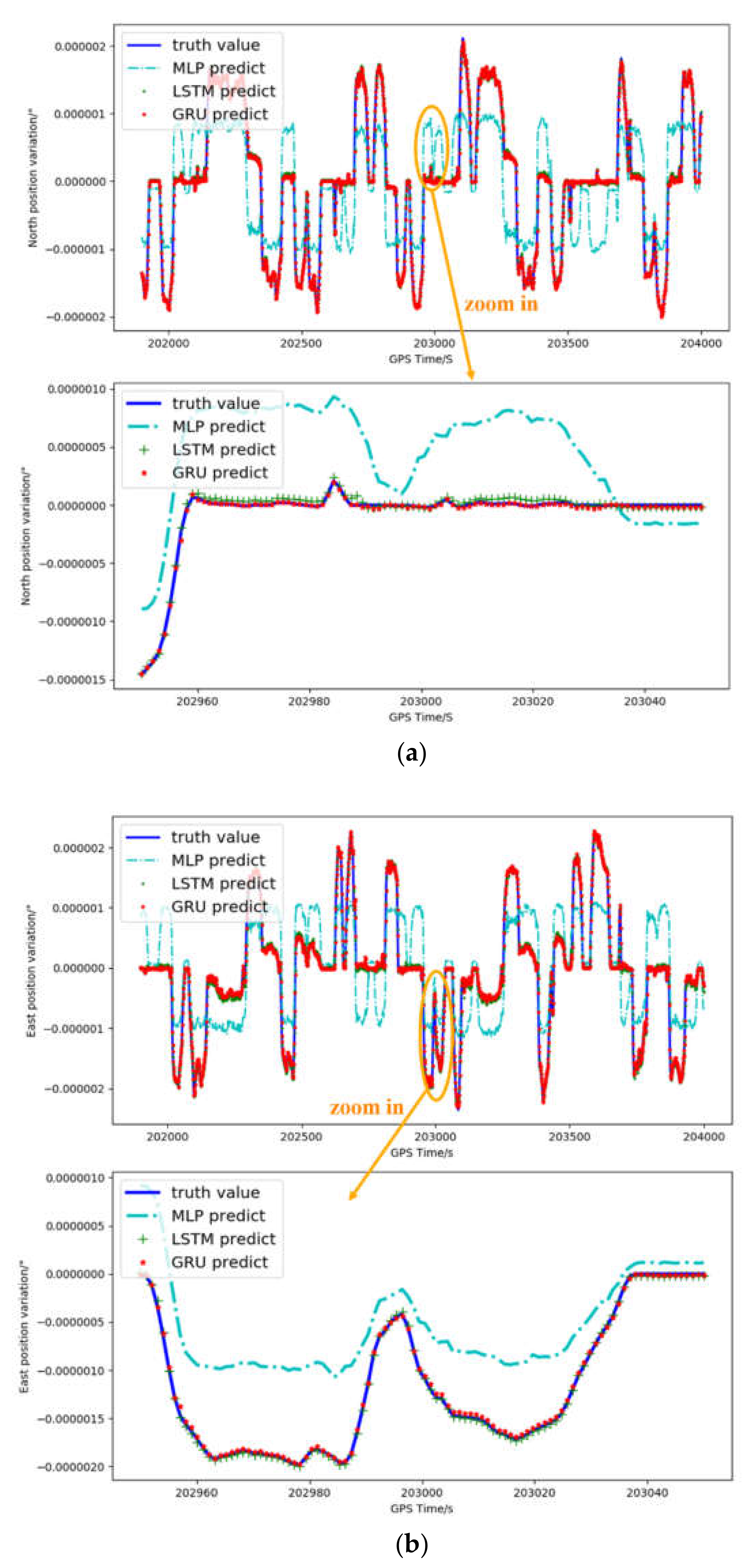
4.1. GRU Prediction Accuracy

The GRU network prediction accuracy was verified with the 2200 s (GPS time: 201,900–204,100 s) test dataset. Meanwhile, an LSTM network and MLP network were constructed as comparison groups. The LSTM network consisted of an LSTM layer with 128 neurons and a fully connected layer activated by the sigmoid function, and the time step was set as 4. The MLP network consisted of 128 neurons but without the time step parameter. The truth value was acquired by SPAN-CPT, and the predicted position variation root mean square error (RMSE) values of the different networks are summarized in

Table 3. The predicted position variation RMSE of the different networks.

	North RMSE/rad	East RMSE/rad
GRU	3.05 × 10−8	3.04 × 10−8
LSTM	3.24 × 10−8	4.96 × 10−8
MLP	6.49 × 10−7	6.81 × 10−7

. The prediction RMSE values of the GRU, LSTM, and MLP network in the North direction are 3.05 × 10⁻⁸, 3.24 × 10⁻⁸, and 6.49 × 10⁻⁷, and the RMSE values in the East direction are 3.04 × 10⁻⁸, 4.96 × 10⁻⁸, and 6.81 × 10⁻⁷. It can be concluded that both recurrent networks (LSTM and GRU) have a similar prediction accuracy and visibly surpass the performance of the MLP network. On the other hand, the training time consumption per epoch of GRU and LSTM is 1.90 and 2.19 s and this result verifies that the GRU network surpasses LSTM in efficiency. The comparison results between LSTM and GRU are also consistent with the conclusion of [27].

The North and East position variations in the GRU prediction, LSTM prediction, and MLP prediction and truth value are shown in Figure 5a,b, respectively. As Figure 5 indicates, the predicted value of GRU and LSTM identifies the truth value while the MLP-predicted value obviously differs from the truth value.

Figure 6 shows the GRU-, LSTM-, and MLP-predicted horizontal trajectory, which is an integral value of the predicted position variation. More specifically, the below trajectory reflects the change in the position of each epoch relative to the starting point (GPS time: 201,900 s, latitude: 30.44681283°, longitude: 114.461966°). As shown in Figure 6, the starting points of the predicted curves are consistent with that of the reference curve, and then the prediction position error accumulates gradually. The reason for this phenomenon is that the predicted position variation, namely ΔP_GNSS, inevitably includes error, and the prediction error, which is positively related to the measurement noise, can accumulate while the ΔP_GNSS is integrated into pseudo P_GNSS, thus it is necessary to adopt AKF to estimate the pseudo GNSS measurement noise matrix.

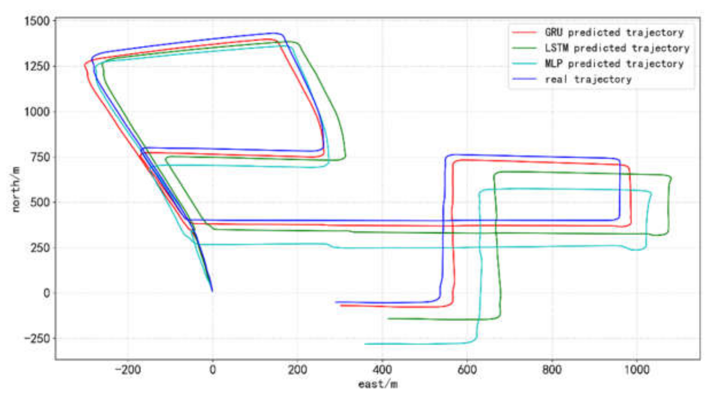
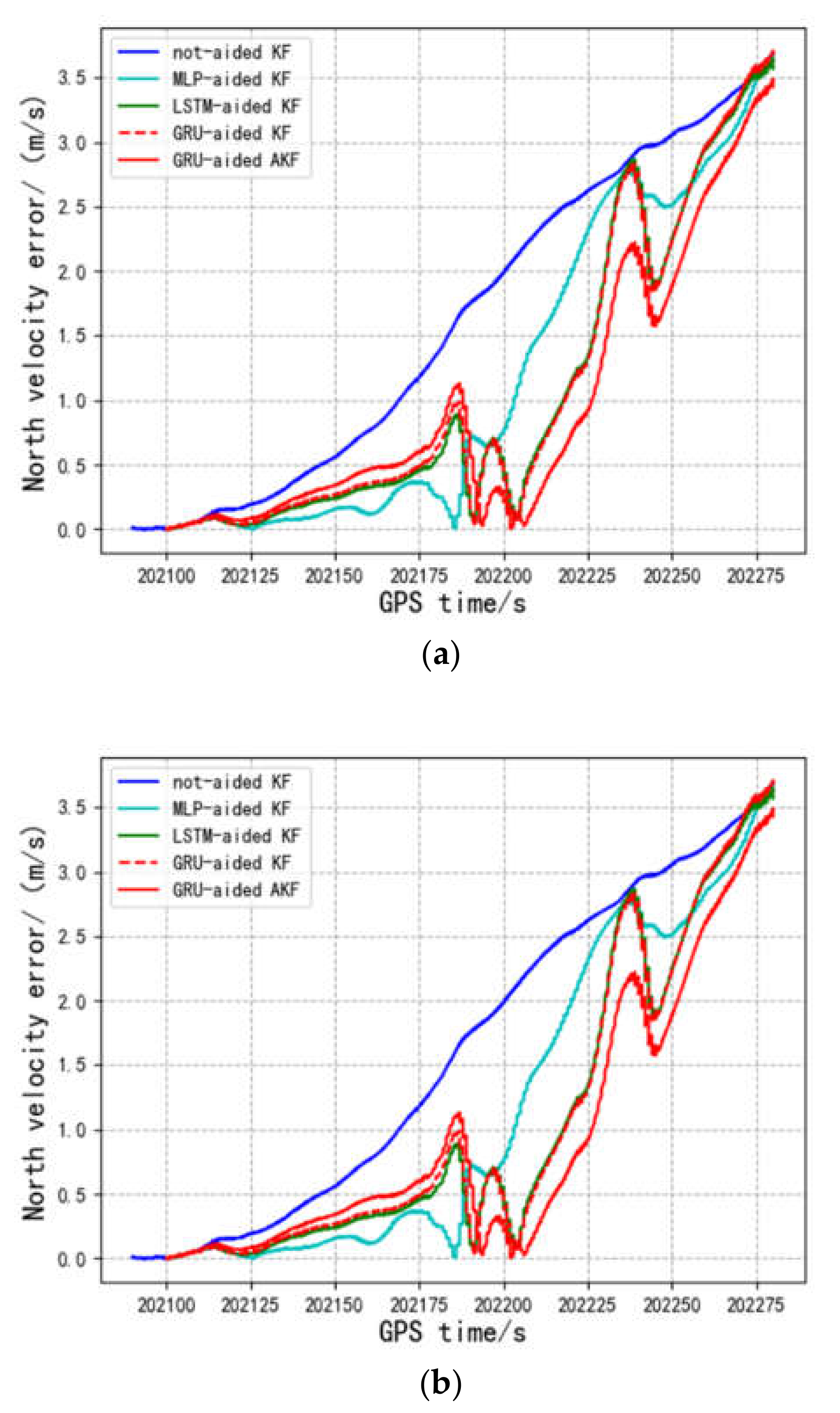
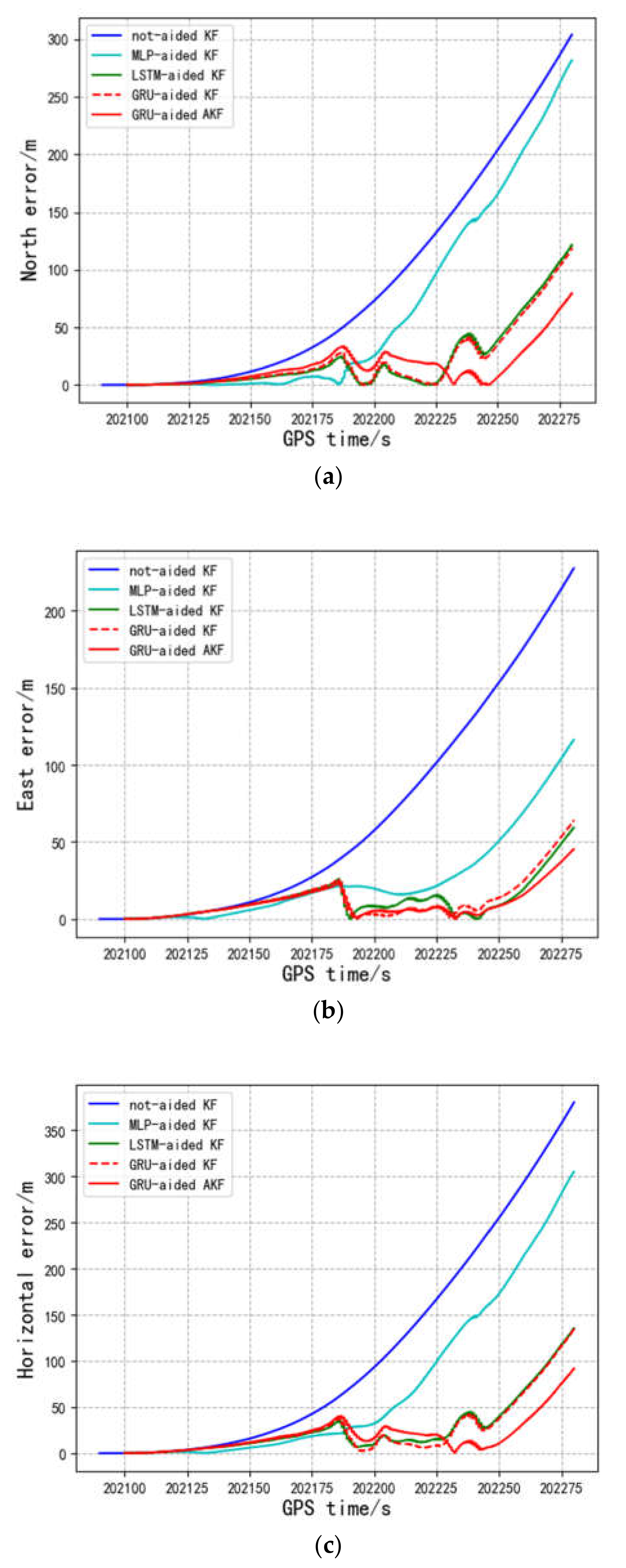
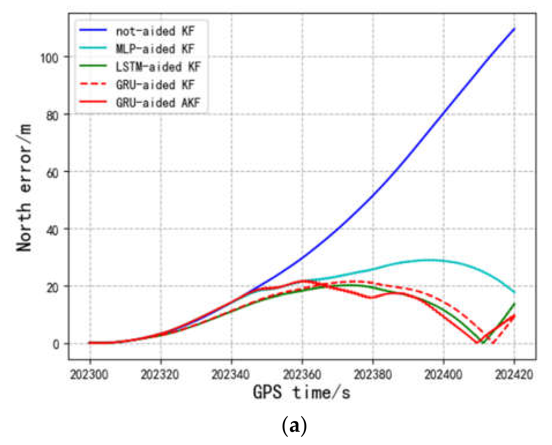
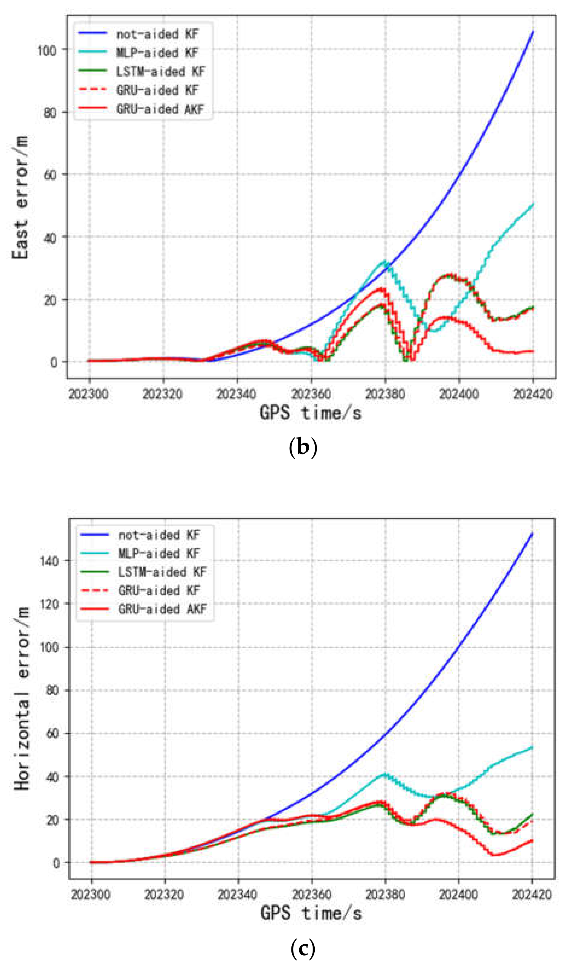
4.2. Integrated Navigation Accuracy

In order to verify the performance of the GRU-aided AKF algorithm, a period of 180 s (GPS time:202,100–202,280 s) and a period of 120 s (GPS time: 202,300–202,420) were selected from the test dataset to simulate a GNSS outage. The position information derived from the proposed GRU network replaces the real GNSS information in the measurement update process of AKF and KF. Meanwhile, the LSTM-aided KF, MLP-aided KF, and not-aided KF were also adopted as control groups.

As is shown in Figure 7, the MLP, LSTM, and GRU network could suppress the velocity error accumulation in both the North and East directions. The maximum velocity errors in the North and East directions estimated by the above-mentioned algorithm are summarized in

Table 4. Maximum velocity errors after 180 s GNSS outage.

	North Velocity Error	East Velocity Error
Not-aided KF	3.691 m/s	2.764 m/s
MLP-aided KF	3.653 m/s	2.688 m/s
LSTM-aided KF	3.570 m/s	2.393 m/s
GRU-aided KF	3.627 m/s	2.352 m/s
GRU-aided AKF	3.430 m/s	1.750 m/s

. Compared with the not-aided KF, MLP-aided and LSTM-aided KF, and GRU-aided KF methods, the proposed GRU-aided AKF reduced the maximum North velocity error by 7.071%, 6.105%, 3.922%, and 5.431%, and the maximum east velocity error by 36.686%, 34.896%, 26.87%, and 25.595%.

Figure 8 shows a comparison of the North, East, and horizontal errors of different algorithms during the 180 s GNSS outage. It is illustrated in Figure 8 that the LSTM-aided KF and GRU-aided KF have almost the same position error during the 180 s GNSS outage, and the GRU network is a better choice due to its higher efficiency. Meanwhile, the GRU-aided AKF’s prediction accuracy exceeds that of the GRU-aided KF after the 120 s GNSS outage, and it can be concluded that the proposed GRU-aided AKF is better suited to a long period of GNSS outage.

The maximum position errors and position error RMS during the 180 s GNSS outage are summarized in

Table 5. Position errors after the 180 s GNSS outage.

	Maximal North Error	Maximal East Error	Maximal Horizontal Error	Horizontal Error RMS
Not-aided KF	303.866 m	227.599 m	379.652 m	157.182 m
MLP-aided KF	281.452 m	116.134 m	304.471 m	113.758 m
LSTM-aided KF	120.761 m	59.109 m	134.452 m	40.062 m
GRU-aided KF	117.314 m	63.462 m	133.379 m	39.232 m
GRU-aided AKF	78.949 m	45.294 m	91.019 m	26.680 m

. The quantitative analysis indicates that the proposed GRU-aided AKF algorithm reduced the maximal horizontal error by 76.03%, 70.10%, 32.30%, and 31.76%, and the horizontal error RMS by 83.03%, 76.55%, 33.40%, and 31.99% compared with the Not-aided, MLP-aided, LSTM-aided, and GRU-aided KF, respectively. Meanwhile, by comparing the data of the MLP-aided, LSTM-aided, and GRU-aided KF, it can be concluded that both recurrent neural networks, namely the LSTM and the GRU, have a similar positioning accuracy and surpass the performance of MLP.

Figure 9 shows a comparison of the North, East, and horizontal errors of the different algorithms during the 120 s GNSS outage. It is obvious that all of the AI-aided algorithms surpass the no-aided one and all of the recurrent neural network-aided algorithms surpassed the MLP-aided one regarding the positioning accuracy. Besides, it can be observed that the proposed GRU-aided AKF position error curve is lower than that of the control groups.

The maximum position errors and position error RMS during the 120 s GNSS outage are summarized in

Table 6. Position errors after the 120 s GNSS outage.

	Maximal North error	Maximal East Error	Maximal Horizontal Error	Horizontal Eerror RMS
Not-aided KF	109.639 m	105.480 m	152.141 m	64.258 m
MLP-aided KF	28.513 m	30.177 m	53.285 m	27.342 m
LSTM-aided KF	19.990 m	26.512 m	30.291 m	17.294 m
GRU-aided KF	21.227 m	26.467 m	31.532 m	18.015 m
GRU-aided AKF	21.331 m	20.544 m	26.450 m	15.813 m

. The proposed GRU-aided AKF algorithm reduced the maximal horizontal error by 82.65%, 50.36%, 12.68%, and 16.12% and the horizontal error RMS by 75.39%, 42.17%, 8.56%, and 12.22% of the not-aided, MLP-aided, LSTM-aided, and GRU-aided KF, respectively. By comparing the not-aided KF and the proposed GRU-aided AKF horizontal error RMS in Table 5 and Table 6, it can observed that the proposed algorithm reduced the horizon error RMS by 75.39% and 83.03% under the 120 and 180 s GNSS outage respectively. This indicates that the proposed algorithm performs better during longer periods of GNSS outage.

5. Discussion

The main advantages of the GRU and AKF hybrid algorithm can be summarized as follows: (1) A high efficiency recurrent neural cell with a simple structure, namely the GRU, was chosen to estimate the pseudo position variation. Benefiting from proper neural cell selection and hyperparameter setting, the proposed algorithm possesses superior navigation accuracy and training efficiency. (2) This paper combined the modern artificial intelligence methodology and conventional adaptation theory to improve the navigation accuracy during GNSS outage. The experiment results under different time scales indicate that the hybrid algorithm surpasses the stand-along adaptive and AI methods.

Meanwhile, further improvements of this work are summarized as follows: (1) The algorithm is currently run on PC and cannot satisfy the real-time dynamic navigation requirement. A potential solution is to integrate the AI chip and the embedded platform. The integrated computational platform could support the proposed method, and has lower power and less volume advantages compared with PC. (2) The training and testing dataset could not cover all the application scenarios, and the GRU network should be trained with more different types of data. As the amount of training data grows, the proposed algorithm will acquire better applicability and adaptability.

6. Conclusions

Aiming to improve the positioning accuracy of INS/GNSS integrated navigation during GNSS outage, this study proposed a GRU and AKF-based integrated navigation algorithm. Owing to proper neural cell selection and hyperparameter setting, the constructed GRU network has a higher prediction accuracy and higher training efficiency. Furthermore, the proposed algorithm introduces adaptive KF to reduce the position error by estimating the GRU prediction error dynamically. Compared with the standard KF-based integrated navigation algorithm, the test results show that the hybrid algorithm reduces the root mean square error by 83.03% and 75.39% and the maximum position error by 76.03% and 82.65% during the 180 and 120 s GNSS outage, respectively. The algorithm can improve the navigation accuracy at different time scales, and has real-time navigation application potential due to its high efficiency.

References

1. Godha, S.; Cannon, M.E. GPS/MEMS INS Integrated System for Navigation in Urban Areas. GPS Solut. 2007, 11, 193–203. [Google Scholar] [CrossRef]
2. Xiao, Y.; Luo, H.; Zhao, F.; Wu, F.; Gao, X.; Wang, Q.; Cui, L. Residual Attention Network-Based Confidence Estimation Algorithm for Non-Holonomic Constraint in GNSS/INS Integrated Navigation System. IEEE Trans. Veh. Technol. 2021, 70, 11404–11418. [Google Scholar] [CrossRef]
3. Grewal, M.S.; Weill, L.R.; Andrews, A.P. Global Positioning Systems, Inertial Navigation, and Integration; John Wiley: Hoboken, NJ, USA, 2001. [Google Scholar]
4. Jiang, H.; Shi, C.; Li, T.; Dong, Y.; Li, Y.; Jing, G. Low-cost GPS/INS Integration with Accurate Measurement Modeling Using an Extended State Observer. GPS Solut. J. Glob. Navig. Satell. Syst. 2021, 25, 17. [Google Scholar] [CrossRef]
5. Wang, D.; Dong, Y.; Li, Z.; Li, Q.; Wu, J. Constrained MEMS-Based GNSS/INS Tightly Coupled System with Robust Kalman Filter for Accurate Land Vehicular Navigation. IEEE Trans. Instrum. Meas. 2020, 69, 5138–5148. [Google Scholar] [CrossRef]
6. Wang, S.Z.; Zhan, X.Q.; Zhai, Y.W.; Chi, C.; Liu, X.Y. Ensuring High Navigation Integrity for Urban Air Mobility Using Tightly Coupled Gnss/Ins System. J. Aeronaut. Astronaut. Aviat. 2020, 52, 429–441. [Google Scholar]
7. Kim, Y.; An, J.; Lee, J. Robust Navigational System for a Transporter Using GPS/INS Fusion. IEEE Trans. Ind. Electron. 2018, 65, 3346–3354. [Google Scholar] [CrossRef]
8. Basar, T. A New Approach to Linear Filtering and Prediction Problems. In Control Theory: Twenty-Five Seminal Papers (1932–1981); IEEE: Piscataway, NJ, USA, 2001; pp. 167–179. [Google Scholar]
9. Priyanka, A. Mems-Based Integrated Navigation; Gnss Technology and Applications Series; Artech House: Boston, MA, USA, 2010. [Google Scholar]
10. Yue, Z.; Lian, B.; Gao, Y. Robust Adaptive Filter Using Fuzzy Logic for Tightly-Coupled Visual Inertial Odometry Navigation System. IET Radar Sonar Navig. 2020, 14, 364–371. [Google Scholar] [CrossRef]
11. Li, T.; Zhang, H.; Gao, Z.; Niu, X.; El-Sheimy, N. Tight Fusion of a Monocular Camera, MEMS-IMU, and Single-Frequency Multi-GNSS RTK for Precise Navigation in GNSS-Challenged Environments. Remote Sens. 2019, 11, 610. [Google Scholar] [CrossRef] [Green Version]
12. Sun, R.; Yang, Y.; Chiang, K.-W.; Duong, T.-T.; Lin, K.-Y.; Tsai, G.-J. Robust IMU/GPS/VO Integration for Vehicle Navigation in GNSS Degraded Urban Areas. IEEE Sens. J. 2020, 20, 10110–10122. [Google Scholar] [CrossRef]
13. Wang, M.; Tayebi, A. Hybrid Nonlinear Observers for Inertial Navigation Using Landmark Measurements. IEEE Trans. Autom. Control 2020, 65, 5173–5188. [Google Scholar] [CrossRef] [Green Version]
14. Li, N.; Guan, L.; Gao, Y.; Du, S.; Wu, M.; Guang, X.; Cong, X. Indoor and Outdoor Low-Cost Seamless Integrated Navigation System Based on the Integration of INS/GNSS/LIDAR System. Remote Sens. 2020, 12, 3271. [Google Scholar] [CrossRef]
15. Schütz, A.; Sánchez-Morales, D.E.; Pany, T. Precise Positioning through a Loosely-Coupled Sensor Fusion of Gnss-Rtk, Ins and Lidar for Autonomous Driving. In Proceedings of the 2020 IEEE/ION Position, Location and Navigation Symposium (PLANS), Portland, OR, USA, 20–23 April 2020. [Google Scholar]
16. Batista, P.; Petit, N.; Silvestre, C.; Oliveira, P. Further Results on the Observability in Magneto-Inertial Navigation. In Proceedings of the 2013 American Control Conference, Washington, DC, USA, 17–19 June 2013; pp. 2503–2508. [Google Scholar]
17. Zhu, K.; Guo, X.; Jiang, C.; Xue, Y.; Li, Y.; Han, L.; Chen, Y. MIMU/Odometer Fusion with State Constraints for Vehicle Positioning during BeiDou Signal Outage: Testing and Results. Sensors 2020, 20, 2302. [Google Scholar] [CrossRef] [Green Version]
18. Ran, C.; Cheng, X. A Direct and Non-Singular Ukf Approach Using Euler Angle Kinematics for Integrated Navigation Systems. Sensors 2016, 16, 1415. [Google Scholar] [CrossRef] [PubMed] [Green Version]
19. Dissanayake, G.; Sukkarieh, S.; Nebot, E.; Durrant-Whyte, H. The Aiding of a Low-Cost Strapdown Inertial Measurement Unit Using Vehicle Model Constraints for land Vehicle Applications. IEEE Trans. Robot. Autom. 2001, 17, 731–747. [Google Scholar] [CrossRef] [Green Version]
20. Sun, W.; Yang, Y. BDS PPP/INS Tight Coupling Method Based on Non-Holonomic Constraint and Zero Velocity Update. IEEE Access 2020, 8, 128866–128876. [Google Scholar] [CrossRef]
21. Abdolkarimi, E.S.; Mosavi, M.-R. A Low-Cost Integrated MEMS-Based INS/GPS Vehicle Navigation System with Challenging Conditions Based on an Optimized IT2FNN in Occluded Environments. GPS Solut. 2020, 24, 108. [Google Scholar] [CrossRef]
22. Zhang, Y.; Wang, L. A Hybrid Intelligent Algorithm DGP-MLP for GNSS/INS Integration during GNSS Outages. J. Navig. 2019, 72, 375–388. [Google Scholar] [CrossRef]
23. Doostdar, P.; Keighobadi, J.; Hamed, M.A. INS/GNSS Integration Using Recurrent Fuzzy Wavelet Neural Networks. GPS Solut. 2019, 24, 29. [Google Scholar] [CrossRef]
24. Al Bitar, N.; Gavrilov, A. A New Method for Compensating the Errors of Integrated Navigation Systems Using Artificial Neural Networks. Measurement 2021, 168, 108391. [Google Scholar] [CrossRef]
25. Dai, H.-F.; Bian, H.-W.; Wang, R.-Y.; Ma, H. An INS/GNSS Integrated Navigation in GNSS Denied Environment Using Recurrent Neural Network. Def. Technol. 2020, 16, 334–340. [Google Scholar] [CrossRef]
26. Noureldin, A.; El-Shafie, A.; Bayoumi, M. GPS/INS Integration Utilizing Dynamic Neural Networks for Vehicular Navigation. Inf. Fusion 2011, 12, 48–57. [Google Scholar] [CrossRef]
27. Lu, S.; Gong, Y.; Luo, H.; Zhao, F.; Li, Z.; Jiang, J. Heterogeneous Multi-Task Learning for Multiple Pseudo-Measurement Estimation to Bridge GPS Outages. IEEE Trans. Instrum. Meas. 2021, 70, 1–16. [Google Scholar] [CrossRef]
28. Yao, Y.; Xu, X.; Zhu, C.; Chan, C.-Y. A Hybrid Fusion Algorithm for GPS/INS Integration during GPS Outages. Measurement 2017, 103, 42–51. [Google Scholar] [CrossRef]
29. Fang, W.; Jiang, J.; Lu, S.; Gong, Y.; Tao, Y.; Tang, Y.; Yan, P.; Luo, H.; Liu, J. A LSTM Algorithm Estimating Pseudo Measurements for Aiding INS during GNSS Signal Outages. Remote Sens. 2020, 12, 256. [Google Scholar] [CrossRef] [Green Version]
30. Assad, A.; Khalaf, W.; Chouaib, I. Radial Basis Function Kalman Filter for Attitude Estimation in GPS-Denied Environment. IET Radar Sonar Navig. 2020, 14, 736–746. [Google Scholar] [CrossRef]
31. Jozefowicz, R.; Zaremba, W.; Sutskever, I. An Empirical Exploration of Recurrent Network Architectures. In Proceedings of the 32nd International Conference on International Conference on Machine Learning, Lille, France, 6–11 July 2015; Volume 37, pp. 2342–2350. [Google Scholar]
32. Yan, G.; Weng, J. Principle of Strapdown Inertial Navigation Algorithm and Integrated Navigation; Northwestern Polytechnical University Press: Xi’an, China, 2019. [Google Scholar]
33. Kottath, R.; Poddar, S.; Das, A.; Kumar, V. Window Based Multiple Model Adaptive Estimation for Navigational Framework. Aerosp. Sci. Technol. 2016, 50, 88–95. [Google Scholar] [CrossRef]
34. Yang, Y.; He, H.; Xu, T. Adaptive Robust Filtering for Kinematic Gps Positioning. Acta Geod. Cartogr. Sin. 2001, 30, 293–298. [Google Scholar]
Figure 1. The structure of GRU.
Remotesensing 14 00752 g001
Figure 2. Structure of GRU-aiding INS/GNSS integrated navigation. (a) Training mode; (b) predicting mode
Remotesensing 14 00752 g002
Figure 3. Data acquisition experimental platform.
Remotesensing 14 00752 g003
Figure 4. Dataset collection trajectory.
Remotesensing 14 00752 g004
Figure 5. Position variation between GPS time 201,900 and 204,100 s. (a) North position variation; (b) East position variation.
Remotesensing 14 00752 g005
Figure 6. Predicted and real horizontal trajectories.
Remotesensing 14 00752 g006
Figure 7. Velocity errors of 180 s outages estimated by different algorithms. (a) North velocity error; (b) East velocity error.
Remotesensing 14 00752 g007
Figure 8. Position errors of 180 s outages estimated by different algorithms. (a) Latitude position error; (b) longitude position error; (c) horizontal position error.
Remotesensing 14 00752 g008
Figure 9. Position errors of 120 s outages estimated by different algorithms. (a) Latitude position error; (b) longitude position error; (c) horizontal position error.
Remotesensing 14 00752 g009aRemotesensing 14 00752 g009b