A Comparative Analysis of Unmanned Aircraft Systems in Low Altitude Photogrammetric Surveys

Abstract

Comparing photogrammetric performances of four user-grade unmanned aircraft systems (UAS) is the main aim of this paper. This study investigates what is the more suitable UAS for specific applications considering the required scale factor, such as for architectural, environmental and restoration purposes. Some photogrammetric surveys were conducted in a 5 ha area using a Phantom 4 Adv, Mavic 2 Pro, Mavic Air 2 and Mavic Mini 2. These unmanned aircrafts are commercial systems used mainly by private professionals. Some photogrammetric reconstructions were carried out by varying flight altitude and camera settings of the 4 UAS. Structure-from-motion (SfM) algorithms were applied to the images taken from the UASs. The surveys’ quality was analyzed by comparing the ground targets’ coordinates measured on the field with indirect georeferencing through global navigation satellite system (GNSS). Fifty targets were installed and arranged following a kind of regular grid. For each photogrammetric flight, the boundary conditions were maintained the same, as well as the flight trajectories and the ground control point distribution. Altimetric and planimetric residuals were reported and compared for each photogrammetric survey. Using a regular grid of ground targets, the result obtained from Phantom 4 is one order of magnitude better than the ones obtained from the other UASs. Mavic Mini 2 leads to an error average of about 5 cm. Remembering that the Mavic Mini 2 is an ultralight drone (it does not require a pilot’s license), it could significantly reduce costs compared to all the others.

1. Introduction

Structure-from-motion (SfM) photogrammetry is extensively used as a topographic modelling technique [1]. It combines the utility of digital photogrammetry and ease of use of multiview computer vision methods [2]. Thanks to the increasing availability of imagery, particularly from unmanned aerial vehicles, SfM photogrammetry represents a powerful tool [3]. Unmanned aircraft systems (UASs), commonly named drones, are gaining more and more importance in the world panorama of photogrammetric surveys [4,5,6]. Some typical applications are for architectural, archaeological, cultural heritage purposes [7], regional planning or risk analysis and mapping [8,9,10].

Due to the technical improvements and miniaturization of avionics and quality advancements of digital cameras, UASs have been increasingly used as remote sensing platforms [11,12].

SfM photogrammetric processing plays an increasing role in delivering digital elevation models (DEMs) from UAS-based imagery [13]. Several commercial software, such as Agisoft Metashape [14], Meshroom [15] and 3DF Zephyr [16], offer automated photogrammetric reconstruction routines. Investigating photogrammetric error and the uncertainties associated with SfM photogrammetric results are crucial tasks [17].

Mapping with unmanned aerial vehicles (RPASs) typically involves the deployment of ground control points (GCPs) to georeference the images and generate topographic models [18]; the photogrammetric process needs support and control points to be able to scale and to georeference the model. Recently, UAS have been equipped with GNSS real-time kinematic (RTK) or post-processed kinematic (PPK) modes that allow georeferencing almost without support or control points, with a pseudo-direct georeferencing method [19,20]. However, we performed indirect georeferencing [21,22,23] as the tested vehicles do not support GNSS RTK.

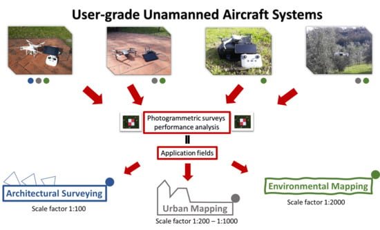
Depending on the type of representation that a performed topographic survey must deliver, a specific type of instrument can be adopted for the survey. For architectural drawing, for instance, 1:50 or 1:100 graphical outputs have often been used [24,25]. For other applications, such as vast landscape, landslides or riverbeds surveying, smaller than 1:1000 graphical scales have been used [26,27,28,29]. This study considers scale factors smaller than 1:100 only; to achieve a 1:50 scale factor, a planimetric error of less than 1 cm must be guaranteed and it is generally out of the range of drones. Nowadays, CAD software or digital maps allow for almost infinite enlargements, and the graphical error is still the parameter that governs measurement accuracy based on the client’s requests. For example, to return the survey on a scale of 1:1000, where the graphic error is ±20 cm, it will not be necessary to go up to an accuracy of less than 5 cm, as this would only involve a waste of energy and unnecessary costs. In photogrammetric topographic surveys from UASs, some authors have worked on scale ranging from 1:3000 [27] to 1:100 [28]. Obtaining a product on a scale greater than 1:100 is not possible with the RTK mode [28]; for this reason, the considerations were carried out starting from the scale factor 100. The altimetric error can be traditionally considered double in topography compared to the planimetric one. The required threshold value on the Z coordinate in three dimensions can be regarded as equal to twice that imposed on planimetric axes. Considering results from the resulting accuracy on a cartographic representation, some considerations can also be made. It represents the uncertainty associated with the graphically represented information; historically, ±0.2 mm has been the minimum distinguishable value with the human eye without a lens. In general, the graphic error depends on the scale of the map, and the tolerances for cartographic purposes are equal to double the graphical error.

Recalling that the ground sampling distance represents the size of the pixel on the field and is a function of the focal length of the camera, flight altitude and size of the sensor’s pixel, it is a parameter that sets a lower limit to the precision achievable on the points on the ground. The GSD value of the 80 m height above ground level (AGL) flight of the Phantom 4 Adv is 2.1 cm.

Tuning the choice of an appropriate surveying technique, considering the expected result in terms of graphical output, could help optimize the campaign costs and find a good balance between available resources and expected outcomes.

Integrating a GNSS control network and photogrammetric technique to design, implement and perform a rigorous topographic survey methodology has been depicted [29,30,31].

The quality of a 3D model mainly depends on the survey’s quality and the photogrammetric reconstruction process. The survey’s quality, in terms of accuracy, is dependent on various parameters: method, performances of UAS avionics, quality of cameras, the accuracy of GNSS observations [32], camera calibration [33,34,35] and the georeferencing method [36].

This paper extends the investigation performed in other publications [37,38,39], bringing under observation two new UAS models.

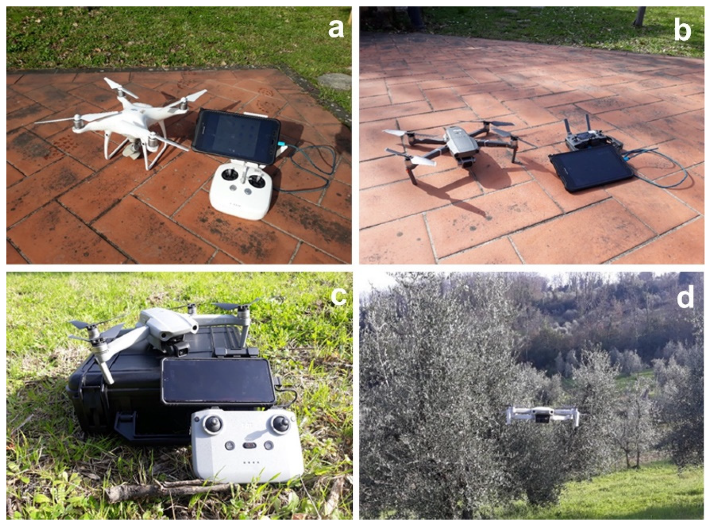
This research has been carried out to investigate outcomes of a series of photogrammetric surveys performed through four DJI UAS models: the Phantom 4 Adv, Mavic 2 Pro, Mavic Air 2 and Mavic Mini 2. Predominant national and international regulations are increasingly favoring small drones in urban areas [40,41,42]. For this reason and considering a wide variety of urban applications for restoration purposes, we focused the tests on small-weight drones. The aircrafts are commercial user grade systems primarily used by private professionals. On the one hand, thanks to their off-the-shelf configurations, they can help in rapidly planning and performing low-altitude surveys.

On the other hand, due to their extraordinary easy-to-use vocation, they are often deployed while paying little attention to photogrammetric best practices. Following these considerations, the tests were designed to reproduce common critical issues such as poor planning of camera network geometry, camera autocalibration and different flighting AGLs.

The tested UASs in different configurations achieved different overall mission performance and survey quality.

2. Materials and Methods

• UAS

Four off-the-shelf consumer-grade UASs, namely, the Phantom 4 Adv, Mavic 2 Pro, Mavic Air 2 and Mavic Mini 2, were used (Figure 1).

In

Table 1. UASs’ technical specifications.

UAS Model	Phantom 4	Mavic 2 Pro	Mavic Air 2	Mavic Mini 2
Image Sensor Type	1 in. CMOS	1 in. CMOS	$\frac{1}{2}$ in. CMOS	$\frac{1}{2.3}$ in. CMOS
Pixel Size	3.1 µm	2.4 µm	0.8 µm	1.5 µm
FOV	84°	77°	84°	83°
Focal Length	24 mm	28 mm	24 mm	24mm
Optical Aperture	f/2.8–f/11	f/2.8–f/11	f/2.8	f/2.8
Shooting Distance	1 m to ꝏ	1 m to ꝏ	1 m to ꝏ	1 m to ꝏ
ISO Range	100–12,800	100–12,800	100–3600	100–12,800
Satellite Systems	GPS + GLONASS	GPS + GLONASS	GPS + GLONASS	GPS/GLONASS/GALILEO

, the main UASs’ specifications are reported.

• GNSS receiver

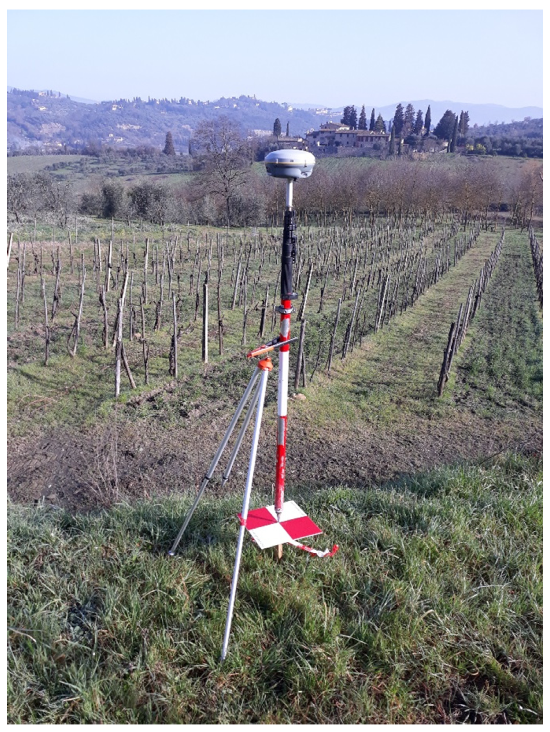
The used GNSS receiver was the TRIMBLE R8s (Figure 2) system with a 2 m high pole and bipod support to guarantee a steady equilibrium during acquisitions. The observations were made in real time kinematic (RTK) mode with area correction receiving nearest station (NEA) corrections from NETGEO’s (www.netgeo.it, accessed on 22 October 2021) permanent network (NRTK) [42]. A number of satellites higher than 12 were verified for each positioning, which was carried out with 3 acquisitions of 10 epochs each. In order to easily integrate the performed survey with other technical maps, the European Terrestrial Reference System ETRS89 in planar representation TM32 on the terrestrial reference frame ETRF2000 was chosen.

The three measured values were averaged, and the resulting value was considered as a reference on which to perform both the checks and the photogrammetric frames. A 1.5 cm error for altimetric and 0.8 cm for planimetric measurements were considered.

• SfM Software

The SfM technique was implemented through automated photogrammetric reconstruction routines. Concerning the photogrammetric reconstruction, Agisoft Metashape’s professional version (1.6.6), was used. The software product works through a standardized processing pipeline: structure-from-motion automatic processing to image block orientation (Figure 3), generating a 3D point cloud of the acquired scene, causing a triangular mesh from the point cloud, creating raster products such as a digital elevation model (DEM) and orthophotos. As a first step, the images were imported without camera specifications and were filtered following a quality threshold. By applying exchangeable image file (EXIF) georeferencing information, the software tool then estimated interior and exterior parameters. GCPs and CkPs were measured trough a GNSS receiver and manually selected on the project images as a second step, in which 51 targets were selected. The GCPs were then selected as a constraint during the bundle block adjustment (BBA) procedure to put the photogrammetric reconstruction within a local coordinate system. CkPs were selected as check points. Once the bundle adjustment processes had been performed, exterior and interior camera parameters were adjusted accurately. A comparison between GCPs and CkPs model coordinates and the coordinates observed by the GNSS survey was performed to assess georeferencing process accuracy. The accuracy was expressed in pixels and meters. The root-mean-square error was calculated for the GCPs and CkPs to better depict the error distribution in the overall study area.

2.1. Surveying Campaign

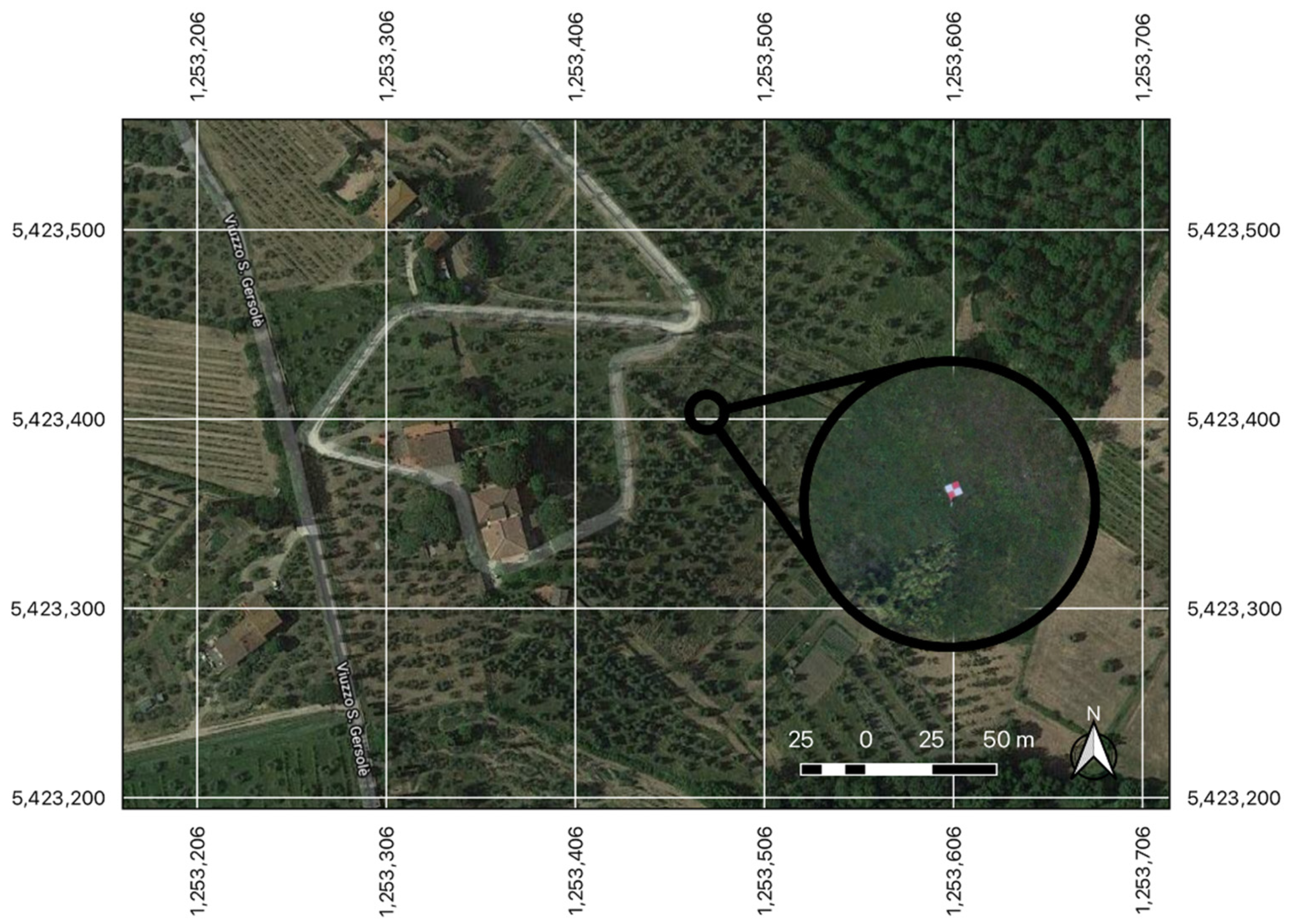
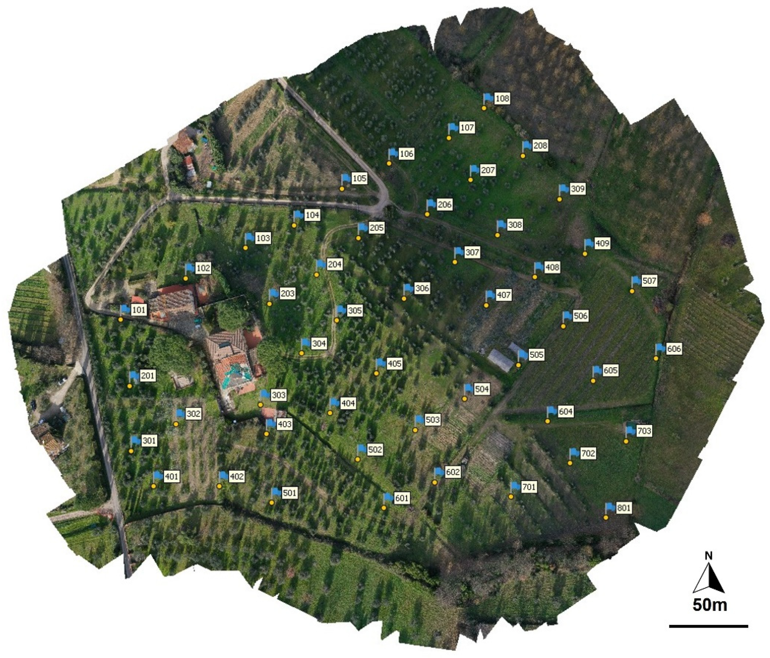
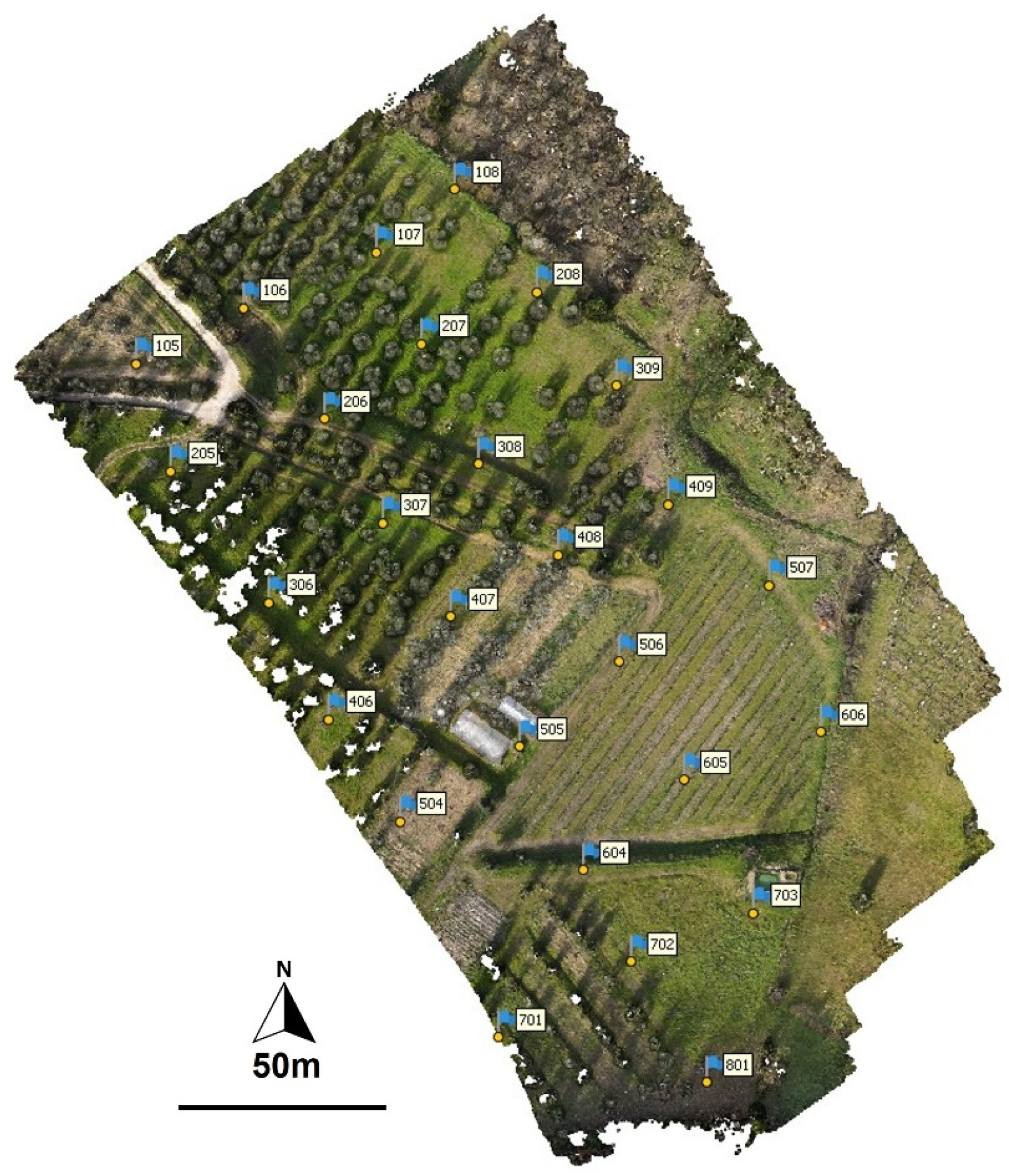
The performance of the various drones was investigated, flying over an inclined terrain. The surveying campaign was performed within three days. During the first two days, the target arrangement and GNSS survey were performed. The photogrammetric flights were carried out during the third day to maintain a reasonable stability of boundary conditions such as wind, temperature, humidity, and cloud coverage. 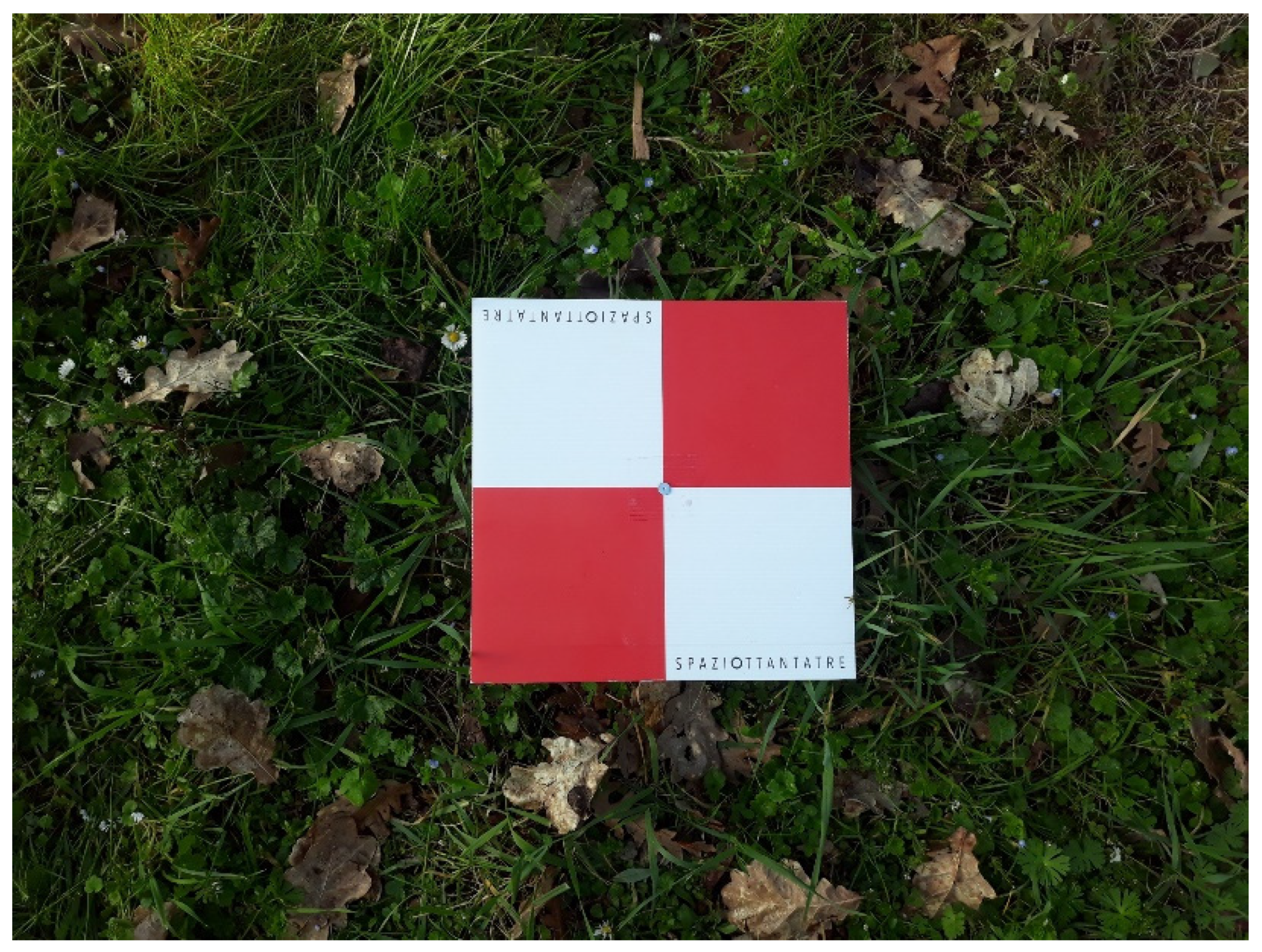The flights were carried out over a portion of land, including an olive grove, a vineyard, and some buildings (Figure 3). Fifty-one targets of size 0.3 × 0.3 m (Figure 4) were positioned on the ground based on a relatively regular grid and fixed on the ground using stable anchoring supports.

Furthermore, a topographic nail was solidly secured in each target’s center, allowing for an accurate GNSS survey. The targets’ coordinates were measured with GNSS observations using a 2 m stick. The observations made through local area correction with a local station were performed stationing on each point for three acquisitions of 10 epochs each. The average value of the three observations was considered for each GCP. An instrumental altimetric error of 15 mm and a 7 mm planimetric error were considered. The coordinates were transformed using a local grid and framed in the EPSG 3003 reference system (Gauss–Boaga west fuse). The targets (Figure 5) have been used as ground control points (GCPs) and check points (CkPs) to improve and verify the quality of the photogrammetric reconstruction.

2.2. Performing the Surveys

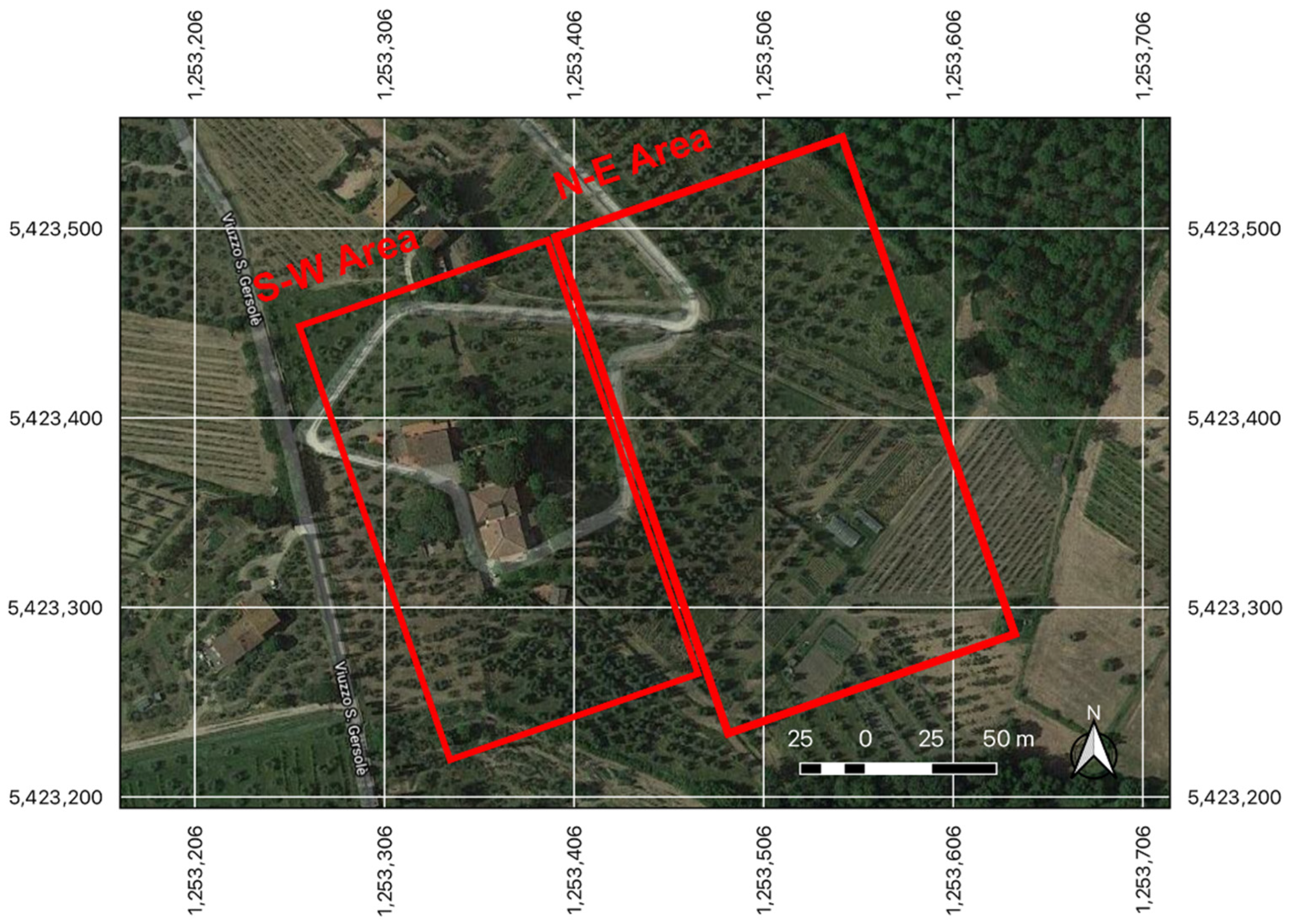
The surveys were performed using the four UAS models described in the previous section. A regular speed and a comparable overall flying dynamic were adopted to guarantee a more stable flight. In particular, the surveying operations were performed using the automatic flight mode for the Phantom 4 Adv and Mavic 2 Pro. For the Mavic Air 2 and Mavic Mini 2, the manual mode was used as the mission planning software was not available. The flying AGL was maintained constant both in manual and automatic missions. However, a flight chart was used during flying operations to maintain the same route followed by the automatic flights and the same speed. This way, the overlapping images were held close to the ones obtained through the automatic flight mode. The study area was divided into southwest and northeast (Figure 6) sections to reduce the error due to the slope inclination.

The complete area coverage was performed, planning two missions for each UAS, one for each area. The UAS performance for different ground sampling distances (GSD) was investigated in terms of photogrammetric efficiency, performing flights at four different AGLs for each mission. For the Phantom 4 Adv and Mavic 2 Pro, flights were performed at 30, 45, 60, and 80 m AGLs (

Table 2. UAS’ performed flight missions for different AGLs.

	Height above the Ground AGL (m)
	30	45	60	80
	GSD (cm)
Phantom 4 Adv	0.8	1.3	1.8	2.4
Mavic 2 Pro	0.8	1.2	1.6	2.1
Mavic Air 2	0.5	0.8	1.1	1.4
Mavic Mini 2	1	1.6	2.1	2.8

). For logistical reasons, for the Mavic Air 2 and Mavic Mini 2, the flights were carried out at 30 and 60 m only.

Table 2 reports the ground sampling distance on the ground for each UAS and for various flying heights. Values were calculated following Equation (1):

$$X_{GSD}=\frac{H}{f}\times x_{img}$$

(1)

where $X_{GSD}$ is the GSD, H is the flying height, f is the focal length and $x_{img}$ is the sensor pixel size.

A 60% side overlap and 80% forward overlap were adopted as optimal configuration for processing images with Metashape software.

3. Results

The following results were obtained performing flights at pre-established AGLs (30, 45, 60, 80 m) with a nearly regular GCPs grid on the ground for each UAS.

• Phantom 4 and Mavic 2 Pro

For the Phantom 4 Adv and Mavic 2 Pro, the whole study area was considered; for the Mavic Air 2 and Mavic Mini 2, only the NE area was considered. The shorter distance between two consecutive GCPs was about 40 m. For the Phantom 4 Adv and Mavic 2 Pro, which covered the whole study area, 27 GCPs and 22 CkPs were comprised in the survey. For the Mavic Air 2 and Mavic Mini 2 that covered the NE area only, there were only 15 GCPs and 12 CkPs.

In

Table 3. Residuals on GCP and CkP for the survey made by the Phantom 4 Adv at different AGLs. Total represents the total error of the 3 components.

UAS	AGL (m)	Target	X Error (m)	Y Error (m)	Z Error (m)	XY Error (m)	Total (m)
Phantom 4 Adv	30	GCP	0.009	0.010	0.012	0.014	0.018
		CkP	0.011	0.010	0.018	0.015	0.023
	45	GCP	0.009	0.010	0.011	0.014	0.018
		CkP	0.011	0.010	0.015	0.015	0.021
	60	GCP	0.100	0.011	0.013	0.015	0.019
		CkP	0.013	0.009	0.018	0.015	0.023
	80	GCP	0.010	0.012	0.013	0.016	0.020
		CkP	0.012	0.012	0.018	0.017	0.024

, GCPs’ and CkPs’ residuals are calculated on the photogrammetric reconstruction made by Phantom 4 Adv’s images. The worst case is represented for the 80 m AGL. The higher residual value is lower than 0.025 m.

Figure 7 reports the residuals for the Z, Y, X axes and 30, 45, 60, 80 AGL meters for the Phantom 4 Adv. The values reported in the chart for each flight AGL represent the error on the CkPs.

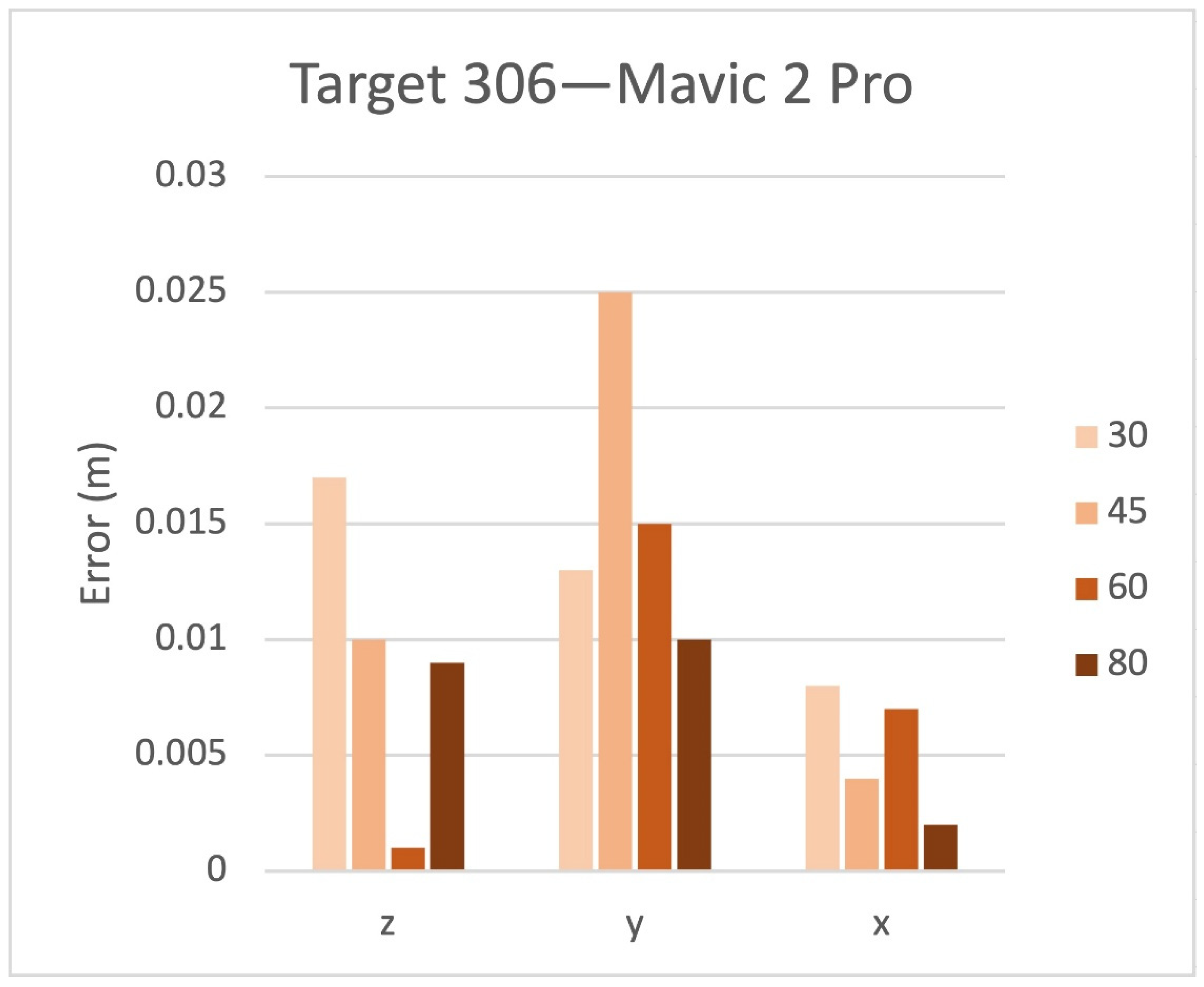
In comparison with the Phantom 4 Adv, the Mavic 2 Pro led to worse results. The total deviation varied from 55.6 cm at 30 m to 18.9 cm at 60 m. The best results were obtained at 60 and 80 m AGL. In addition, the average deviations on the ground control point and checkpoint can be considered homogeneous in this situation.

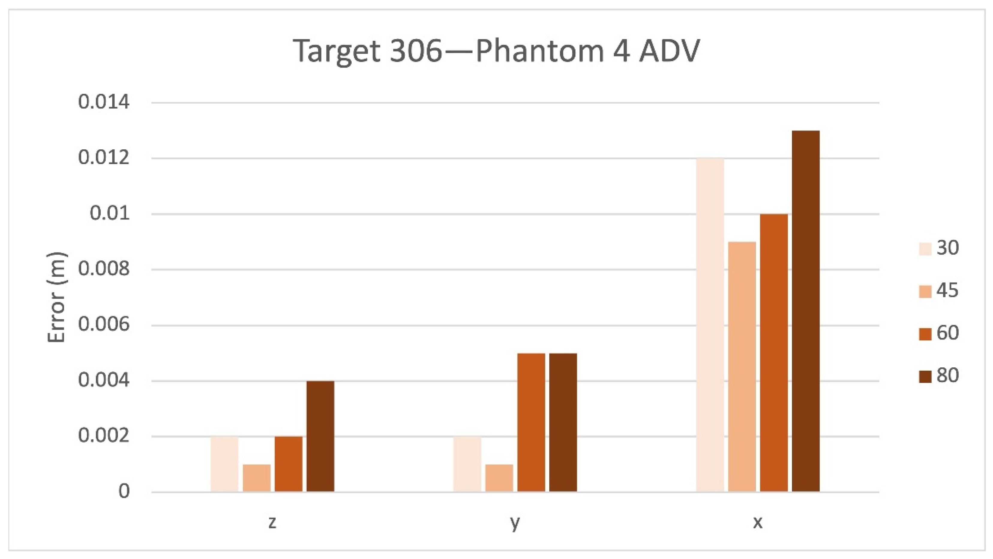
Attention was placed on targets 306 and 406, from which it can be observed again how the vertical component of the error is prevalent (

Table 4. Residuals on GCP and CkP for the survey made by the Mavic 2 Pro at different AGLs. Total represents the total error of the 3 components.

Drone	Altitude (m)	Target	X Error (m)	Y Error (m)	Z Error (m)	XY Error (m)	Total (m)
Mavic 2 Pro	30	GCP	0.029	0.034	0.024	0.045	0.051
		CkP	0.143	0.180	0.505	0.230	0.556
	45	GCP	0.043	0.044	0.025	0.061	0.066
		CkP	0.107	0.099	0.140	0.146	0.202
	60	GCP	0.031	0.031	0.024	0.044	0.050
		CkP	0.075	0.096	0.145	0.122	0.189
	80	GCP	0.026	0.027	0.029	0.037	0.047
		CkP	0.073	0.081	0.193	0.109	0.222

).

Figure 8 reports the residuals for the Z, Y, X axes and 30, 45, 60, 80 AGL meters for the Mavic 2 Pro on target 306. The values reported in the chart for each flight AGL represent errors on the CkPs.

• Mavic Air 2 and Mavic Mini 2

In this case, the surveys were carried out within the northwest area only (Figure 9). Two targets, 308 and 408, belonging to the central part of the survey area were randomly chosen to compare different flights and different UASs.

Table 5. Residuals on GCP and CkP for the survey made by the Mavic Air 2 Adv at different AGLs. Total represents the total error of the 3 components.

Drone	AGL (m)	Target	X Error (m)	Y Error (m)	Z Error (m)	XY Error (m)	Total (m)
Mavic Air 2	30	GCP	0.030	0.059	0.117	0.066	0.135
		CkP	0.032	0.085	0.255	0.091	0.270
	60	GCP	0.066	0.089	0.096	0.111	0.147
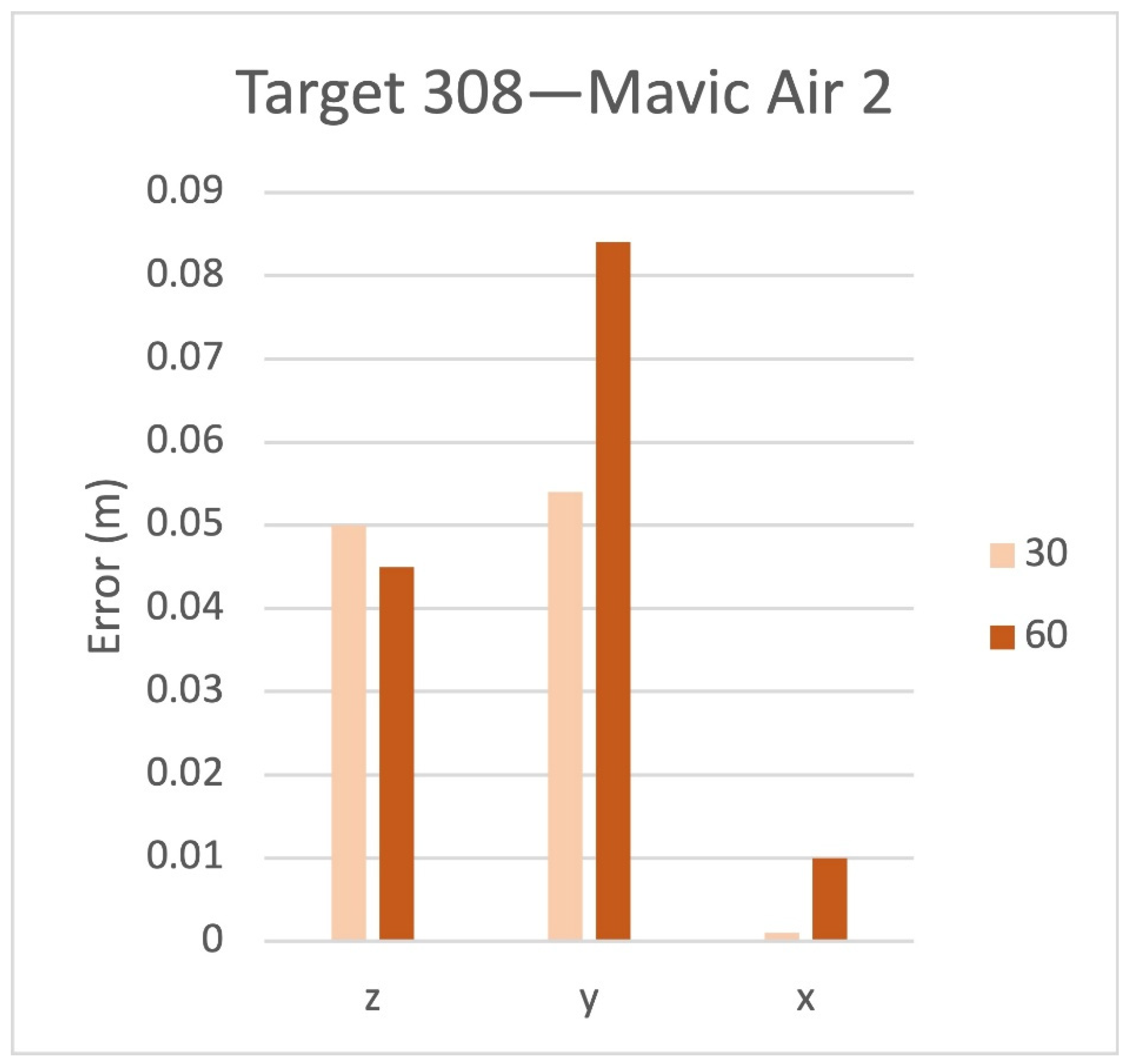
		CkP	0.062	0.109	0.174	0.126	0.215

and Figure 10 summarize the residuals in the X, Y, Z axes measured during a photogrammetric survey made by the Mavic air 2.

Table 6. Residuals on GCP and CkP for the survey made by the Mavic Mini 2 Adv at different AGLs. Total represents the total error of the 3 components.

Drone	AGL (m)	Target	X Error (m)	Y Error (m)	Z Error (m)	XY Error (m)	Total (m)
Mavic Mini 2	30	GCP	0.024	0.032	0.043	0.040	0.058
		CkP	0.025	0.053	0.077	0.058	0.097
	60	GCP	0.022	0.024	0.037	0.033	0.049
		CkP	0.017	0.035	0.055	0.038	0.067

and Figure 11 summarize the residuals in the Z, Y, X axes measured during a photogrammetric survey made by the Mavic air 2.

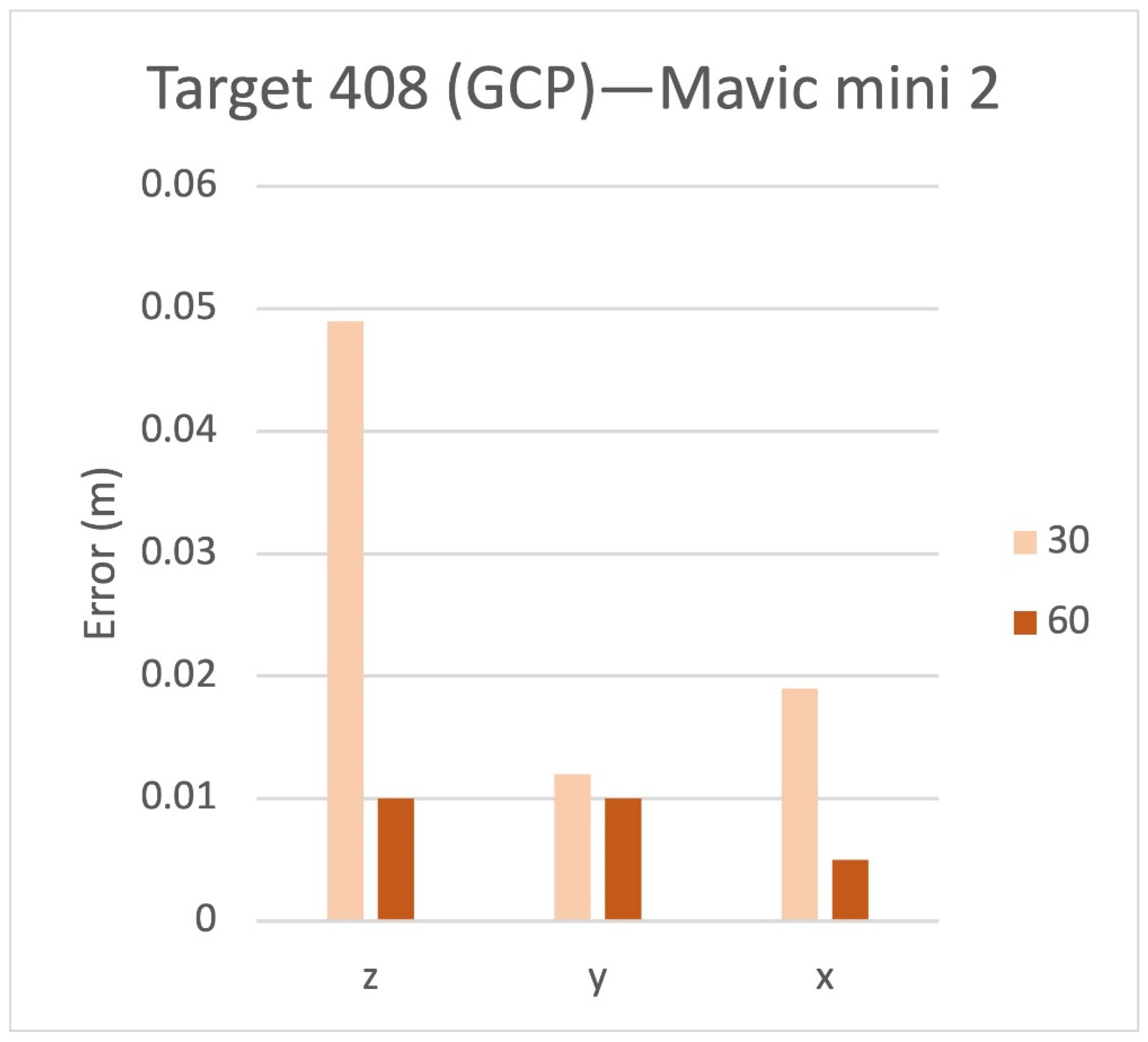
The Mavic Mini 2, unlike the Mavic Air 2, despite its relatively small size and weight (<250 g), has interesting results. The deviations calculated from the photogrammetric reconstruction show a good potential, especially in the case of flying at 60 m, where the errors are even lower than the Mavic 2 Pro.

Hereafter a comparison of residuals for 60 m AGL flights of the four UASs is shown (

Table 7. Residuals for 60 m AGL flights for all the UAS models. Total represents the total error of the 3 components.

Drone	Target	X Error (cm)	Y Error (cm)	Z Error (cm)	XY Error (cm)	Total (cm)
Phantom 4 Adv	GCP	0.9	1.1	1.2	1.4	1.9
	CkP	1.2	0.9	1.7	1.6	2.3
Mavic 2 Pro	GCP	4.1	4.3	1.7	6.0	6.3
	CkP	4.0	3.6	2.1	5.4	5.8
Mavic Air 2	GCP	5.7	8.3	7.2	10.0	12.4
	CkP	6.0	8.5	11.9	10.4	15.8
Mavic Mini 2	GCP	2.2	2.3	3.6	3.2	4.8
	CkP	1.8	3.2	4.7	3.6	5.9

).

All things considered, the average residuals from the Phantom 4 Adv, about 15 mm, almost disappear compared to the other UASs; the discrepancy is one order of magnitude. We can even assert that the Mavic Air 2, limited to the proposed set up and to the border conditions on which the tests were performed, could be difficult to use for topographic survey purposes. The average error was around 10 mm. The Mavic 2 Pro and the Mavic Mini 2 show similar planimetric residuals. The Mavic 2 Pro is better for elevation error; however, the Mavic Mini 2 demonstrated good performance, which represents the most surprising result from this UASs comparison. With a regular grid geometry of ground targets, the Mavic Mini 2 led to an average error of about 5 cm. Remembering that the Mavic Mini 2 is an ultralight drone (it does not require a pilot’s license), it could significantly reduce costs compared to all the others.

4. Discussions

The Phantom 4 Adv brought excellent results for the four analyzed flight AGLs.

The errors reported for the three axes were around 2 cm. With a minimal variance, we can say that values were similar for all ground targets; the point clouds were closely settled around the GCP allowing for the same CkP accuracy.

Two targets belonging to the central part of the survey area were chosen to make a more immediate comparison amongst different flights made by different UASs: GCP 306 and CkP 406.

The prevailing error was the planimetric one; on target 406 (CkP), the predominant deviation was in the vertical direction Z. This statement was valid on targets 306 and 406 and at a general level on all GCPs and CkPs. Furthermore, it is possible to see how the 80 m AGL led to slightly worse results than the other flight AGLs, which can be considered similar in terms of obtained results.

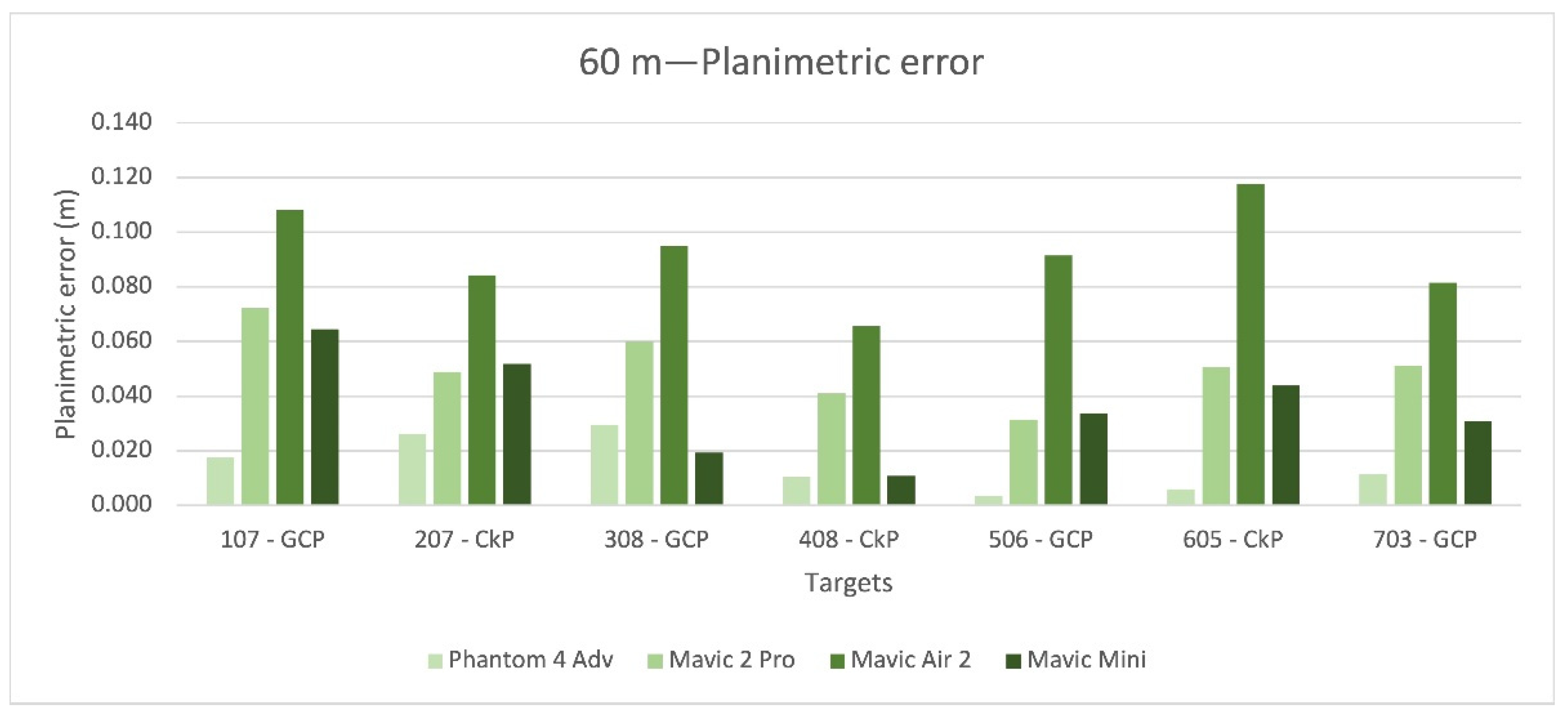
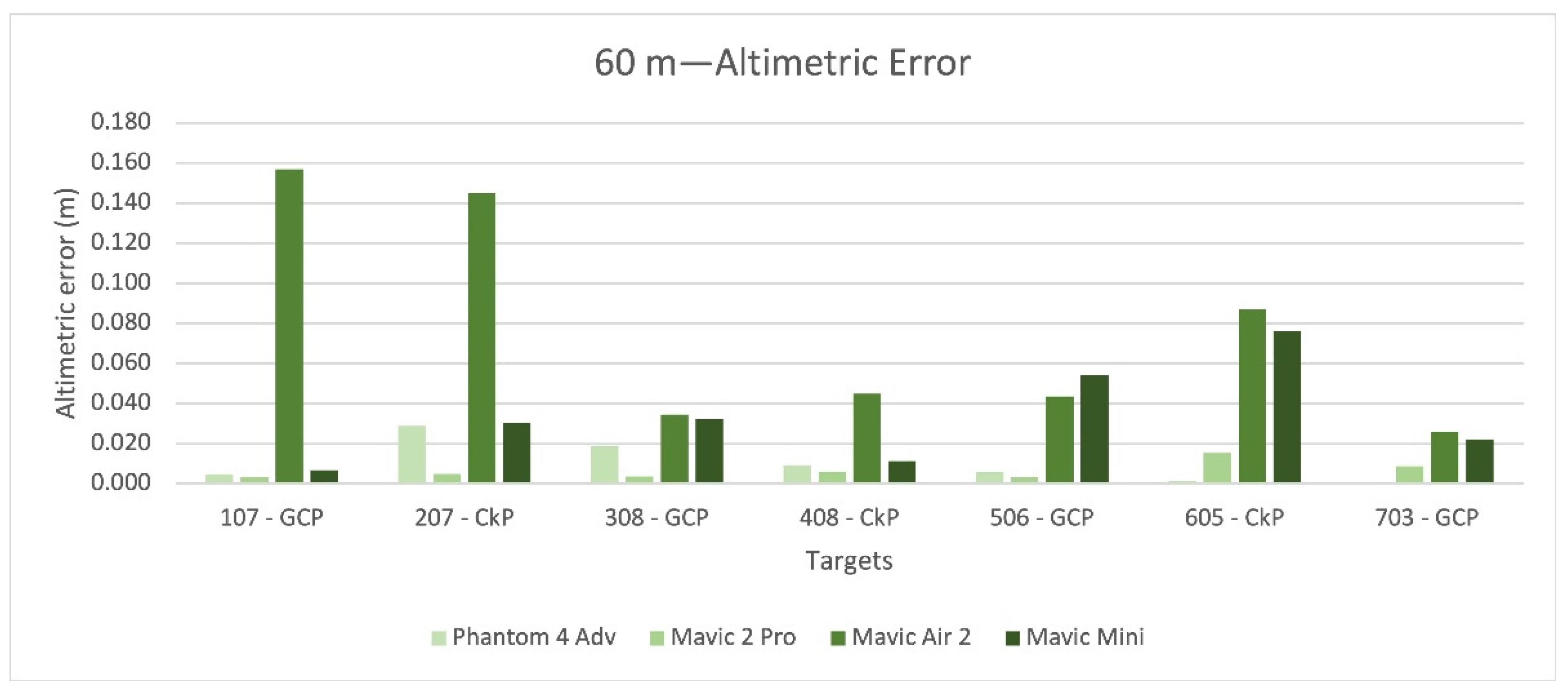
A targets’ single raw image of the ground target grid was chosen to carry out a general comparison of the targets, formed by a GCP (107, 308, 506, 703) and a CkP (207, 408, 605), alternately. As previously highlighted, the geometry of the ground points’ grid ensures that there were no significant differences between GCP and CkP. Figure 12 shows the planimetric deviations on the targets; in Figure 13, the altimetric deviations are represented.

Table 8. Median calculated for the planimetric error.

	Median—Planimetric Error (m)			Kurtosis Index—Planimetric Error
	CkP	GCP	Total	CkP	GCP	Total
Phantom 4 Adv	0.010	0.014	0.011	0.676	1.225	0.564
Mavic 2 Pro	0.049	0.055	0.051	−0.244	−0.504	−0.447
Mavic Air 2	0.084	0.093	0.091	1.076	−0.105	0.308
Mavic Mini 2	0.044	0.032	0.034	0.341	−0.433	0.648

,

Table 9. Median calculated for the altimetric error.

	Median—Altimetric Error (m)			Kurtosis Index—Altimetric Error
	CkP	GCP	Total	CkP	GCP	Total
Phantom 4 Adv	0.009	0.005	0.006	−0.271	0.766	0.273
Mavic 2 Pro	0.006	0.004	0.005	0.478	1.344	−0.447
Mavic Air 2	0.087	0.039	0.045	−0.690	1.719	0.229
Mavic Mini 2	0.030	0.027	0.030	0.847	−1.321	1.673

,

Table 10. Standard deviation calculated for the planimetric error.

	STD—Planimetric Error
	CkP	GCP	Total
Phantom 4 Adv	0.011	0.011	0.010
Mavic 2 Pro	0.005	0.017	0.013
Mavic Air 2	0.026	0.011	0.017
Mavic Mini 2	0.022	0.019	0.019

and

Table 11. Standard deviation calculated for the altimetric error.

	STD—Altimetric Error
	CkP	GCP	Total
Phantom 4 Adv	0.010	0.014	0.008
Mavic 2 Pro	0.004	0.006	0.003
Mavic Air 2	0.054	0.050	0.062
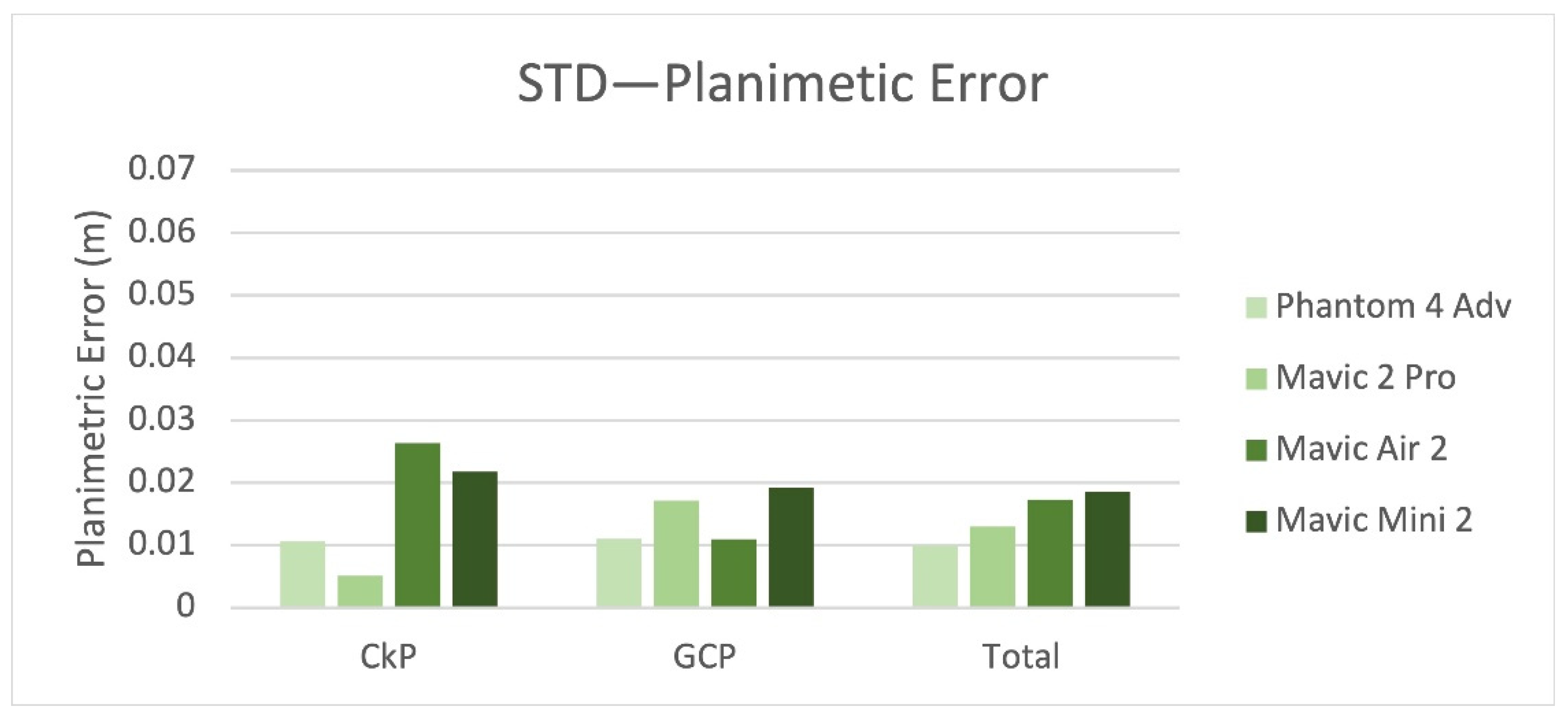
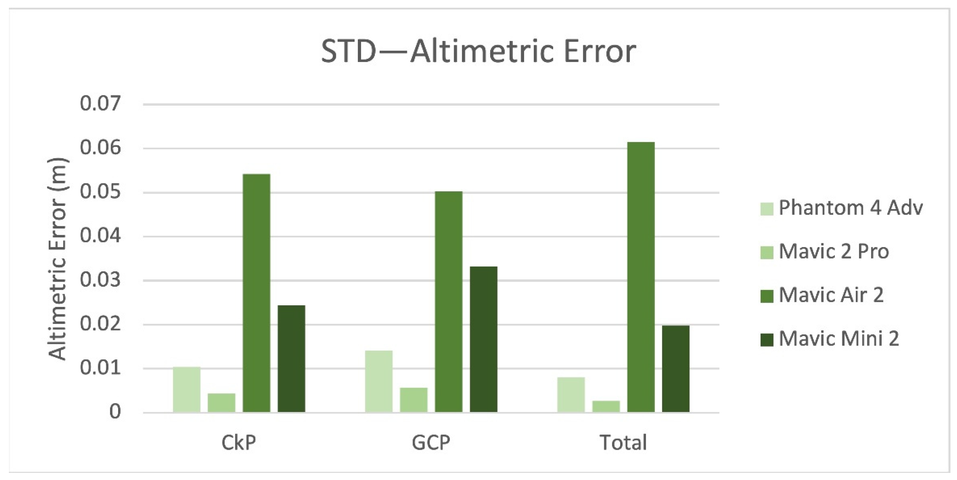
Mavic Mini 2	0.024	0.033	0.020

report the statistics of the survey in terms of median and standard deviation (STD) for planimetric and altimetric errors on the targets GCP (107, 308, 506, 703) and CKP (207, 408, 605). In particular the median, standard deviation and kurtosis index were calculated for GCPs, CkPs, separately, as well as the total amount for the targets.

Table 12. Standard deviation calculated on the planimetric and altimetric errors.

STD—Planimetric Error (m)		STD—Altimetric Error (m)
GCP_All_UAS	CkP_All_UAS	GCP_All_UAS	CkP_All_UAS
0.032	0.032	0.038	0.043
Total
0.031		0.040

shows a STD value for GCPs and CkPs substantially equal for the planimetric error. A slight difference between GCPs and CkPs is otherwise reported for the altimetric error. The total altimetric error is 1 cm higher than the planimetric one.

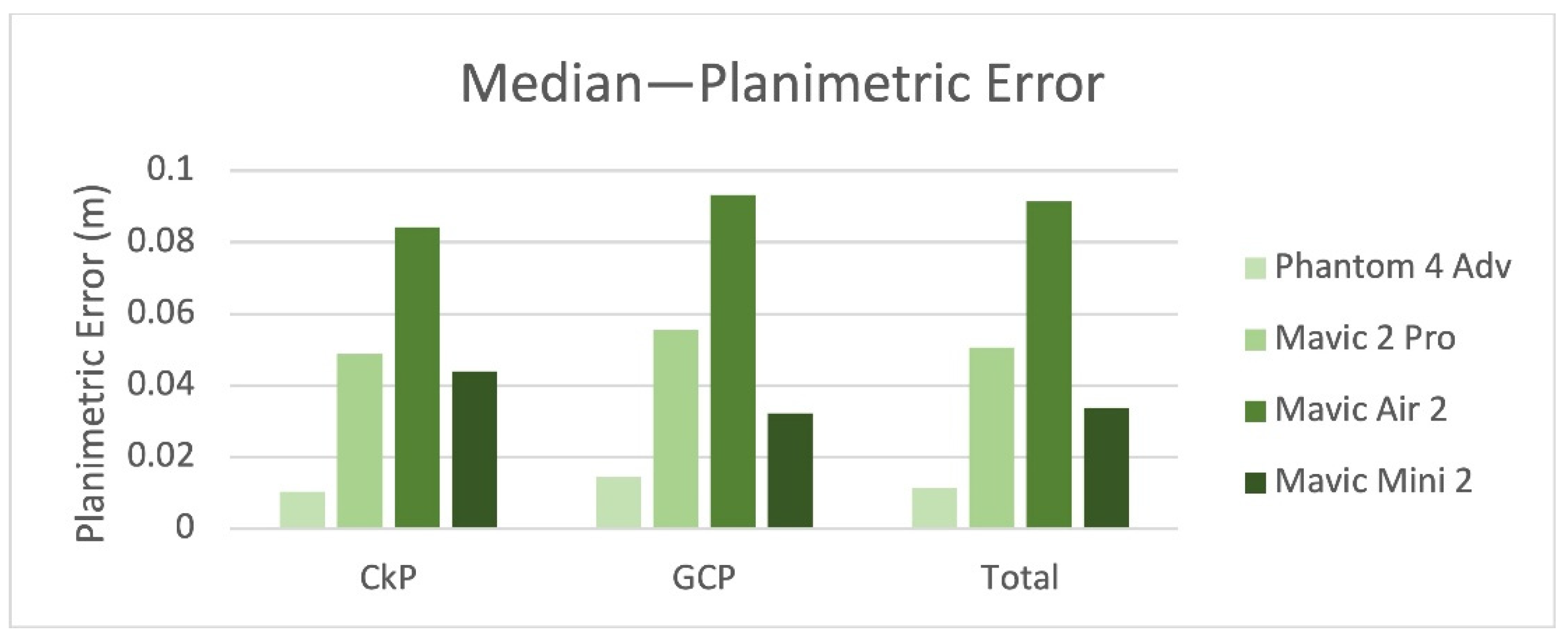
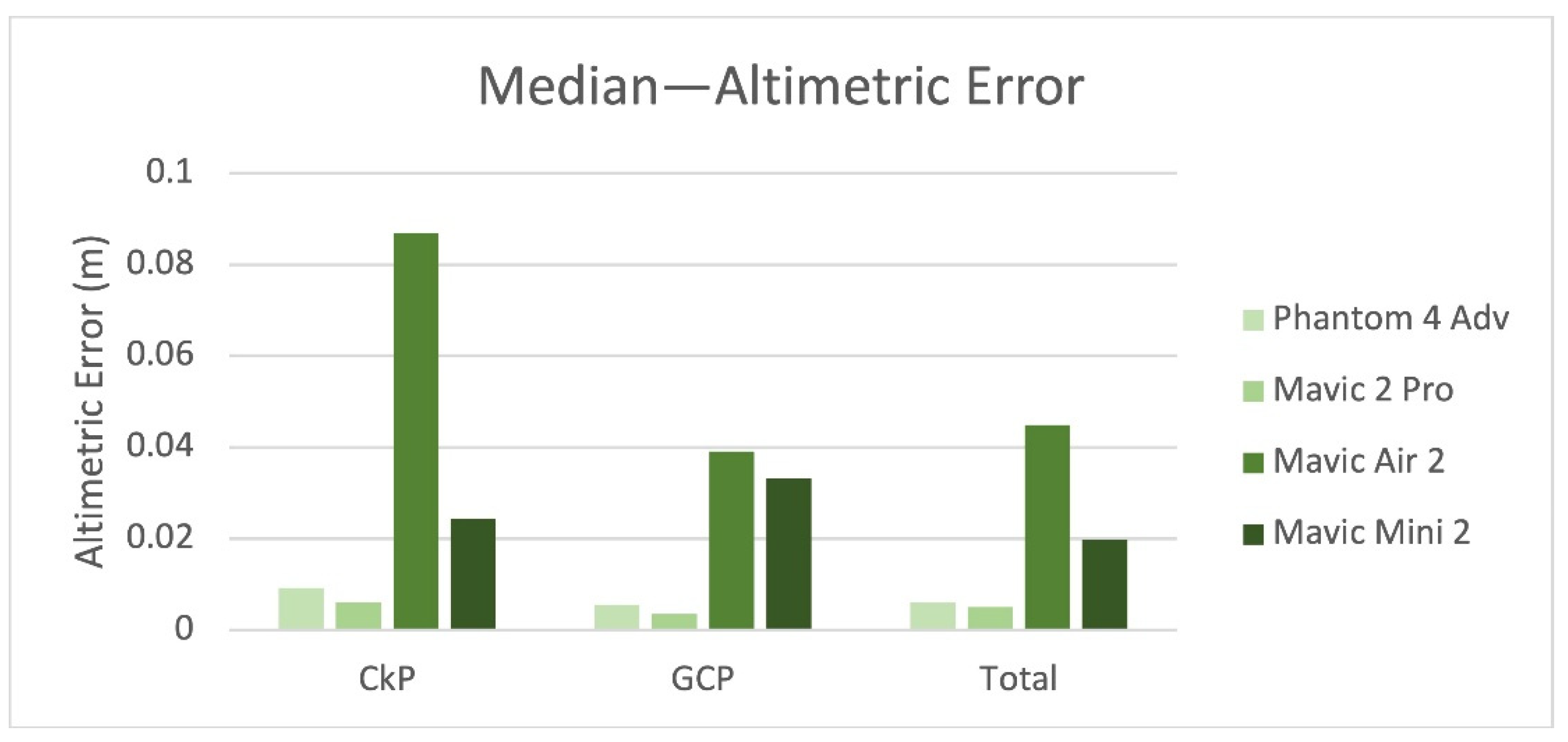
Figure 14 and Figure 15 show the medians for planimetric and altimetric errors on targets GCP (107, 308, 506, 703) and CkP (207, 408, 605). The median value for the altimetric error of the Mavic Air 2 is twice that of the others. Figure 16 and Figure 17 show the standard deviation for the planimetric and altimetric errors on targets GCP (107, 308, 506, 703) and CkP (207, 408, 605). Even in this case, the Mavic Air 2 had worse results.

Table 13. Planimetric graphic errors when performing flights at different AGLs.

Scale	Graphic Error	Phantom 4 Adv	Mavic 2 Pro	Mavic Air 2	Mavic Mini 2
1:100	2 cm	30, 45 m	-	-	-
1:200	4 cm	30, 45, 60, 80 m	-	-	60 m
1:500	10 cm	30, 45, 60, 80 m	30, 45, 60, 80 m	30 m	30, 60 m
1:1000	20 cm	30, 45, 60, 80 m	30, 45, 60, 80 m	30, 60 m	30, 60 m

and

Table 14. Altimetric graphic errors when performing flights at different AGLs.

Scale	Graphic Error	Phantom 4 Adv	Mavic 2 Pro	Mavic Air 2	Mavic Mini 2
1:100	4 cm	30, 45 m	-	-	-
1:200	8 cm	30, 45, 60, 80 m	-	-	-
1:500	20 cm	30, 45, 60, 80 m	30, 45, 60, 80 m	-	30, 60 m

show the flight AGL suitable for a photogrammetric survey, respecting the graphical error limits imposed by the required representation scale and GSD. The values indicate for each drone the flight AGL at which it is possible to fly to ensure the success of a survey at the defined representation scale in terms of planimetric error.

Considering the results from the resulting accuracy on a cartographic representation, some considerations can also be made. It represents the uncertainty associated with the graphically represented information; historically, ±0.2 mm has been the minimum distinguishable value with the human eye without a lens. In general, the graphic error depends on the scale of the map, as shown in

Table 15. Graphic error according to scale factor.

Scale Factor	Graphic Error
1:100	2 × 10−2
1:200	4 × 10−2
1:500	1 × 10−1
1:1000	2 × 10−1
1:2000	4 × 10−1

.

5. Conclusions

Several photogrammetric reconstructions were performed by varying essential parameters such as flight AGL and cameras (RPAS models), applying structure-from-motion (SfM) algorithms using images taken from the UASs. The surveys’ quality was analyzed by comparing the ground targets’ coordinates extrapolated from the point clouds to those measured on the field with indirect georeferencing through GNSS technology.

Looking at the results, the difference between GCPs and CkPs, in terms of error, was moderate. However, although usually the error associated to CkPs should represent the more severe quality control parameter, in this case, for some UAS, the GCP error was higher than the one from the CkPs.

The Phantom 4 Adv confirmed the expectations, being one of the most used drones for photogrammetry. All four flight AGLs used guaranteed accuracy limits to the 1:200 scale. Flight AGLs up to 45 m can generate 1:100 products.

The Mavic 2 Pro cannot assure an acceptable average error for scale factors 100 and 200; however, it was suitable from 1:500 upwards.

The Mavic Air 2 was difficult to use for 1:100 and 1:200 scales. It was within 1:500 at an AGL of 30 m. It is also worth noticing that the sensor is a 48 MP with 2 × 2 binning. With 2 × 2 binning, four adjacent pixels are binned into one larger pixel and readout.

The Mavic Mini 2 exceeded expectations; at a height of 60 m, it could be used for a 1:200 scale. The flight at 60 m resulted in better performance than at 30 m: this could be due to the nonoptimal network camera geometry adopted during the performed surveying. A low signal-to-noise ratio, which is probably due to the sensor size (1/2.3 in. for 12 MP), could even play a role.

From a practical point of view, the Phantom 4 could be the right UAS for various applications such as mapping, urban context and buildings and architectural surveys. The accuracy reached with low AGL missions can also guarantee successful surveys for plans and nondetailed sections. The Mavic 2 Pro, Mavic Air 2 and Mavic Mini 2 can be profitably applied for environmental and urban mapping. Considering UAS regulations [39], in Europe, but also in other countries, thanks to its very low weight (<250 g), the Mavic Mini 2 can be easily used within an urban context and it could be exploited to create robust 3D models in complex scenarios.

References

1. Mancini, F.; Dubbini, M.; Gattelli, M.; Stecchi, F.; Fabbri, S.; Gabbianelli, G. Using unmanned aerial vehicles (UAV) for high-resolution reconstruction of topography: The structure from motion approach on coastal environments. Remote Sens. 2013, 5, 6880–6898. [Google Scholar] [CrossRef] [Green Version]
2. Stott, E.; Williams, R.D.; Hoey, T.B. Ground control point distribution for accurate kilometre-scale topographic mapping using an RTK-GNSS unmanned aerial vehicle and SfM photogrammetry. Drones 2020, 4, 55. [Google Scholar] [CrossRef]
3. James, M.R.; Chandler, J.H.; Eltner, A.; Fraser, C.; Miller, P.E.; Mills, J.P.; Noble, T.; Robson, S.; Lane, S.N. Guidelines on the use of structure-from-motion photogrammetry in geomorphic research. Earth Surf. Process. Landforms 2019, 44, 2081–2084. [Google Scholar] [CrossRef]
4. Malinverni, E.S.; Barbaro, C.C.; Pierdicca, R.; Bozzi, C.A.; Tassetti, A.N. UAV Surveying for a Complete Mapping and Documentation of Archaeological Findings. The Early Neolithic Site of Portonovo. Int. Arch. Photogramm. Remote Sens. Spat. Inf. Sci. 2016, 41, 11149–11155. [Google Scholar]
5. Nex, F. UAV photogrammetry for mapping and 3D modeling–current status and future perspectives. Int. Arch. Photogramm. Remote Sens. Spat. Inf. Sci. 2011, 38, 25–31. [Google Scholar]
6. Waagen, J. New technology and archaeological practice. Improving the primary archaeological recording process in excavation by means of UAS photogrammetry. J. Archaeol. Sci. 2019, 101, 11–20. [Google Scholar] [CrossRef]
7. Lo Brutto, M.; Garraffa, A.; Meli, P. UAV Platforms for Cultural Heritage Survey: First Results. ISPRS Ann. Photogramm. Remote Sens. Spat. Inf. Sci. 2014, II-5, 227–234. [Google Scholar] [CrossRef] [Green Version]
8. Boccardo, P.; Chiabrando, F.; Dutto, F.; Tonolo, F.G.; Lingua, A. UAV deployment exercise for mapping purposes: Evaluation of emergency response applications. Sensors 2015, 15, 15717–15737. [Google Scholar] [CrossRef] [PubMed] [Green Version]
9. Samad, A.M.; Kamarulzaman, N.; Hamdani, M.A.; Mastor, T.A.; Hashim, K.A. The potential of Unmanned Aerial Vehicle (UAV) for civilian and mapping application. In Proceedings of the 2013 IEEE 3rd International Conference on System Engineering and Technology, Shah Alam, Malaysia, 19–20 August 2013; pp. 313–318. [Google Scholar]
10. Bitelli, G.; Balletti, C.; Brumana, R.; Barazzetti, L.; D’urso, M.G.; Rinaudo, F.; Tucci, G. Metric Documentation of Cultural Heritage: Research Directions from the Italian Gamher Project. Int. Arch. Photogramm. Remote Sens. Spat. Inf. Sci. 2017, 42, 2. Available online: https://re.public.polimi.it/handle/11311/1035369 (accessed on 22 October 2021).
11. Turner, D.; Lucieer, A.; Wallace, L. Direct georeferencing of ultrahigh-resolution UAV imagery. IEEE Trans. Geosci. Remote Sens. 2013, 52, 2738–2745. [Google Scholar] [CrossRef]
12. Parisi, E.I.; Suma, M.; Güleç Korumaz, A.; Rosina, E.; Tucci, G. Aerial Platforms (UAV) Surveys in the VIS and TIR Range. Applications on Archaeology and Agriculture. Int. Arch. Photogramm. Remote Sens. Spat. Inf. Sci. 2019, 42, 945–952. [Google Scholar] [CrossRef] [Green Version]
13. James, M.R.; Robson, S. Mitigating systematic error in topographic models derived from UAV and ground-based image networks. Earth Surf. Process. Landforms 2014, 39, 1413–1420. [Google Scholar] [CrossRef] [Green Version]
14. Agisoft Agisoft Metashape Homepage. May 2021. Available online: https://www.agisoft.com (accessed on 22 October 2021).
15. Griwodz, C.; Gasparini, S.; Calvet, L.; Gurdjos, P.; Castan, F.; Maujean, B.; De Lillo, G.; Lanthony, Y. AliceVision Meshroom: An open-source 3D reconstruction pipeline. In Proceedings of the 12th ACM Multimedia Systems Conference, Istanbul, Turkey, 28 September–1 October 2021; pp. 241–247. [Google Scholar]
16. 3DFlow 3D Zephyr. 2021. Available online: https://www.3dflow.net/it/software-di-fotogrammetria-3df-zephyr/ (accessed on 22 October 2021).
17. Agüera-Vega, F.; Carvajal-Ramírez, F.; Martínez-Carricondo, P. Assessment of photogrammetric mapping accuracy based on variation ground control points number using unmanned aerial vehicle. Measurement 2017, 98, 221–227. [Google Scholar] [CrossRef]
18. Hugenholtz, C.; Brown, O.; Walker, J.; Barchyn, T.; Nesbit, P.; Kucharczyk, M.; Myshak, S. Spatial accuracy of UAV-derived orthoimagery and topography: Comparing photogrammetric models processed with direct geo-referencing and ground control points. Geomatica 2016, 70, 21–30. [Google Scholar] [CrossRef]
19. Pfeifer, N.; Glira, P.; Briese, C. Direct georeferencing with on board navigation components of light weight UAV platforms. Int. Arch. Photogramm. Remote Sens. Spat. Inf. Sci. 2012, 39, 487–492. [Google Scholar] [CrossRef] [Green Version]
20. Sanz-Ablanedo, E.; Chandler, J.H.; Rodríguez-Pérez, J.R.; Ordóñez, C. Accuracy of unmanned aerial vehicle (UAV) and SfM photogrammetry survey as a function of the number and location of ground control points used. Remote Sens. 2018, 10, 1606. [Google Scholar] [CrossRef] [Green Version]
21. Eling, C.; Wieland, M.; Hess, C.; Klingbeil, L.; Kuhlmann, H. Development and evaluation of a UAV based mapping system for remote sensing and surveying applications. Int. Arch. Photogramm. Remote Sens. Spat. Inf. Sci. 2015, 40, 233–239. [Google Scholar] [CrossRef] [Green Version]
22. Stöcker, C.; Nex, F.; Koeva, M.; Gerke, M. Quality assessment of combined IMU/GNSS data for direct georeferencing in the context of UAV-based mapping. Int. Arch. Photogramm. Remote Sens. Spat. Inf. Sci. 2017, 42, 355–361. [Google Scholar] [CrossRef] [Green Version]
23. Ekaso, D.; Nex, F.; Kerle, N. Accuracy assessment of real-time kinematics (RTK) measurements on unmanned aerial vehicles (UAV) for direct geo-referencing. Geo-Spat. Inf. Sci. 2020, 23, 165–181. [Google Scholar] [CrossRef] [Green Version]
24. Sun, Z.; Zhang, Y. Using drones and 3D modeling to survey Tibetan architectural heritage: A case study with the multi-door stupa. Sustainability 2018, 10, 2259. [Google Scholar] [CrossRef] [Green Version]
25. Bonora, V.; Maseroli, R.; Mugnai, F.; Tucci, G. GNNs Control Network Supporting Large Historical Building Architectural Survey. Int. Arch. Photogramm. Remote Sens. Spat. Inf. Sci. 2021, 46, 87–91. [Google Scholar] [CrossRef]
26. Mucchi, L.; Jayousi, S.; Martinelli, A.; Caputo, S.; Intrieri, E.; Gigli, G.; Gracchi, T.; Mugnai, F.; Favalli, M.; Fornaciai, A. A flexible wireless sensor network based on ultra-wide band technology for ground instability monitoring. Sensors 2018, 18, 2948. [Google Scholar]
27. Lane, S.N.; James, T.D.; Crowell, M.D. Application of digital photogrammetry to complex topography for geomorphological research. Photogramm. Rec. 2000, 16, 793–821. [Google Scholar] [CrossRef]
28. Barba, S.; Barbarella, M.; Di Benedetto, A.; Fiani, M.; Limongiello, M. Quality Assessment of UAV Photogrammetric Archaeological Survey. Int. Arch. Photogramm. Remote Sens. Spat. Inf. Sci. 2019, 42, 93–100. [Google Scholar] [CrossRef] [Green Version]
29. Gabrlik, P.; la Cour-Harbo, A.; Kalvodova, P.; Zalud, L.; Janata, P. Calibration and accuracy assessment in a direct georeferencing system for UAS photogrammetry. Int. J. Remote Sens. 2018, 39, 4931–4959. [Google Scholar] [CrossRef] [Green Version]
30. Forlani, G.; Diotri, F.; di Cella, U.M.; Roncella, R. Indirect UAV strip georeferencing by on-board GNSS data under poor satellite coverage. Remote Sens. 2019, 11, 1765. [Google Scholar] [CrossRef] [Green Version]
31. Lee, S.; Choi, Y. Comparison of topographic surveying results using a fixed-wing and a popular rotary-wing unmanned aerial vehicle (drone). Tunn. Undergr. Space 2016, 26, 24–31. [Google Scholar] [CrossRef] [Green Version]
32. Fraser, C.S. Automatic camera calibration in close range photogrammetry. Photogramm. Eng. Remote Sens. 2013, 79, 381–388. [Google Scholar] [CrossRef] [Green Version]
33. Remondino, F.; Fraser, C. Digital camera calibration methods: Considerations and comparisons. Int. Arch. Photogramm. Remote Sens. Spat. Inf. Sci. 2006, 36, 266–272. [Google Scholar]
34. Forlani, G.; Dall’Asta, E.; Diotri, F.; di Cella, U.M.; Roncella, R.; Santise, M. Quality assessment of DSMs produced from UAV flights georeferenced with on-board RTK positioning. Remote Sens. 2018, 10, 311. [Google Scholar] [CrossRef] [Green Version]
35. Peppa, M.V.; Hall, J.; Goodyear, J.; Mills, J.P. Photogrammetric assessment and comparison of DJI Phantom 4 pro and phantom 4 RTK small unmanned aircraft systems. In Proceedings of the ISPRS Geospatial Week 2019, Enschede, The Netherlands, 10–14 June 2019. [Google Scholar]
36. Dering, G.M.; Micklethwaite, S.; Thiele, S.T.; Vollgger, S.A.; Cruden, A.R. Review of drones, photogrammetry and emerging sensor technology for the study of dykes: Best practises and future potential. J. Volcanol. Geotherm. Res. 2019, 373, 148–166. [Google Scholar] [CrossRef]
37. Rango, A.; Laliberte, A. Impact of flight regulations on effective use of unmanned aircraft systems for natural resources applications. J. Appl. Remote Sens. 2010, 4, 043539. [Google Scholar]
38. Alamouri, A.; Lampert, A.; Gerke, M. An Exploratory Investigation of UAS Regulations in Europe and the Impact on Effective Use and Economic Potential. Drones 2021, 5, 63. [Google Scholar] [CrossRef]
39. Marshall, D.M. UAS Regulations, Standards, and Guidance. In Introduction to Unmanned Aircraft Systems; CRC Press: New York, NY, USA, 2021; pp. 101–136. [Google Scholar]
40. Nocerino, E.; Menna, F.; Remondino, F.; Saleri, R. Accuracy and block deformation analysis in automatic UAV and terrestrial photogrammetry-Lesson learnt. ISPRS Ann. Photogramm. Remote Sens. Spat. Inf. Sci. 2013, 2, 203–208. [Google Scholar] [CrossRef] [Green Version]
41. Dardanelli, G.; Maltese, A.; Pipitone, C.; Pisciotta, A.; Lo Brutto, M. NRTK, PPP or Static, That Is the Question. Testing Different Positioning Solutions for GNSS Survey. Remote Sens. 2021, 13, 1406. [Google Scholar] [CrossRef]
42. Garilli, E.; Bruno, N.; Autelitano, F.; Roncella, R.; Giuliani, F. Automatic detection of stone pavement’s pattern based on UAV photogrammetry. Autom. Constr. 2021, 122, 103477. [Google Scholar] [CrossRef]
Figure 1. Used UASs: (a) Phantom 4 ADV; (b) Mavic 2 Pro; (c) Mavic Air 2; (d) Mavic Mini 2.
Remotesensing 14 00726 g001
Figure 2. Measuring session of a ground target with pole, GNSS antenna and bipod.
Remotesensing 14 00726 g002
Figure 3. Orthomosaic of the surveyed area.
Remotesensing 14 00726 g003
Figure 4. Ground target.
Remotesensing 14 00726 g004
Figure 5. Sparse point cloud of the study area and GCP regular grid.
Remotesensing 14 00726 g005
Figure 6. South-west and northeast testing areas.
Remotesensing 14 00726 g006
Figure 7. Residuals from the Phantom 4 on CkP 306.
Remotesensing 14 00726 g007
Figure 8. Residuals from the Mavic 2 Pro on CkP 306.
Remotesensing 14 00726 g008
Figure 9. Sparse point cloud of the NW area.
Remotesensing 14 00726 g009
Figure 10. Residuals from the Mavic 2 Pro on CkP 308.
Remotesensing 14 00726 g010
Figure 11. Residuals on CkP 408.
Remotesensing 14 00726 g011
Figure 12. Chart of the residuals on GCPs and CkPs of the four UASs (Planimetric).
Remotesensing 14 00726 g012
Figure 13. Chart of the residuals on GCPs and CkPs of the four UASs (Altimetric).
Remotesensing 14 00726 g013
Figure 14. Chart of median calculated for the planimetric error.
Remotesensing 14 00726 g014
Figure 15. Chart of median calculated for the altimetric error.
Remotesensing 14 00726 g015
Figure 16. Chart of standard deviations calculated for the planimetric error.
Remotesensing 14 00726 g016
Figure 17. Chart of standard deviations calculated for the altimetric error.
Remotesensing 14 00726 g017