1. Introduction
Many different approaches of scattering matrix decomposition have been proposed in the literature in order to extract high quality information from polarimetric data [
1,
2,
3,
4,
5,
6,
7,
8]. Generally, they can be broadly classified into two categories: coherent and non-coherent decompositions. Coherent decomposition methods were developed to characterize completely polarized scattered waves for which fully polarimetric information is contained in the scattering matrix. On the other hand, non-coherent decomposition techniques were developed to characterize a large number of statistically identical scatterers, randomly distributed and with none of them being dominant.
As far as target decomposition is concerned the reader can find in [
1] a thorough analysis of polarimetry and the most significant target decomposition approaches. In this work the H/
α decomposition is emphasized. According to the latter, Cloude and Pottier proposed the representation of scattering characteristics by the space of the entropy H and the averaged scattering angle
α parameters. New roll-invariant scattering-type parameters for both full-polarimetric (FP) and compact-polarimetric (CP) SAR data is presented in [
9]. These provide equivalent information as the Cloude α for FP SAR data and the ellipticity parameter χ for CP SAR data to characterize various targets adequately. A model-free four-component scattering power decomposition that alleviates the compensations of the parameter of the orientation angle about the radar line of sight and the occurrence of negative power components is introduced in [
10]. In [
2] an automatic classification of the dominant scattering mechanisms associated with the pixels of polarimetric SAR images was carried out. Two operating scenarios are investigated. Firstly, it is assumed that the polarimetric image pixels locally share the same covariance (homogeneous environment), and secondly, polarimetric pixels with different power levels and the same covariance structure (heterogeneous environment) are examined. A simple modification was introduced in [
3] which ensures that all covariance matrices in the decomposition will have nonnegative eigenvalues. Systematic approaches of coherent target decomposition (CTD) were presented by Cameron in [
5] proving that the polarimetric responses of the primitive shapes are remarkably stable as the shapes are rotated about various axes. In [
8] the co-diagonalization of the Sinclair backscattering matrix is revisited to overcome the Huynen decomposition issues [
11]. Consequently, scatterer polarimetric properties are correctly extracted leading to the proper selection of the predominant scattering mechanism.
Based on Cameron’s decomposition characterization of polarimetric symmetric scatterers has been proposed by Touzi and Charbonneau in [
12] and used in various types of targets such as permanent scatterers [
13] and ships [
14]. Furthermore, a ship recognition from chaff clouds is carried out in [
15] based on a seven-component model polarimetric decomposition. In [
16] a twofold approach was presented for elementary scattering mechanisms, based on Cameron CTD and applied for automatic ship scatterers characterization. In [
17] the elementary scatterers obtained from Cameron CTD are used as the states of Markov chain models to characterize polarimetric SAR land cover. More than 20 polarimetric decompositions techniques, without including Cameron’s, were used in [
18] to extract a set of polarimetric scattering features, which was optimized in order to improve land cover classification.
The present work relies on Cameron’s coherent decomposition method [
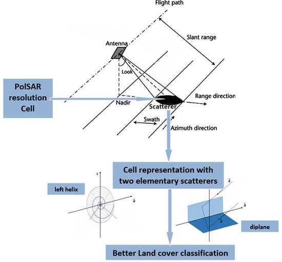
6] and makes further changes and extensions with a view at a more realistic and robust interpretation of the scattering matrix corresponding to a pixel or a resolution cell aiming to collect the highest amount of polarimetric information. According to the method proposed in this manuscript each SAR pixel is characterized by the two most dominant scatterers. This results from the fact that only the four elemental scatterers (trihedral, dipole, dihedral and ¼ wave device) are adequate to extract the available information from each PolSAR cell. These four elementary scatterers, which are in pairs complementary to each other, form the adequate topology to characterize each PolSAR pixel. It is therefore intended to introduce a new sophisticated feature-tool, which will employ most of the available information and will be suitable for application in a wide variety of classification and detection tasks that utilize fully polarimetric data, without being limited by the characterization of coherent or non-coherent technique.
The paper is organized as follows. In
Section 2 the Cameron CTD is described. Moreover, the mapping approach from the unit disk to the unit sphere that is employed to construct the ideal geometric space is explained.
Section 3 contains the reasons for questioning the reliability of the results exported by Cameron’s procedure and introduces our novel approach, based on the two most dominant scatterers. In
Section 4 the employed RADARSAT-2 fully polarimetric SLC data are thoroughly described. In the next section the experimental procedure is explained analytically and the results are presented to validate the proposed method. The conclusions are drawn in
Section 6.
2. Methods—Cameron’s Decomposition and the Symmetric Scatterer Space
Cameron’s CTD analysis [
4,
5] utilizes the Huynen [
11] hypothesis of the two fundamental properties of scatterers, reciprocity and symmetry. A scatterer is reciprocal when the non-diagonal elements of its backscattering matrix are pair-wise equal. The theorem of reciprocity applies to all monostatic SAR systems since the transmitting and receiving antennas share the same location. Therefore, all scatterers are regarded as reciprocal when imaged by monostatic SAR systems. A reciprocal scatterer is symmetric if it presents an axis of symmetry in the plane perpendicular to the radar Line of Sight (LOS).
Cameron’s CTD proceeds as follows, initially the backscattering matrix
is projected onto a basis set where each matrix represents a predominant scattering mechanism. In this case, the aforementioned basis set is a set of matrices proportional to the Pauli matrices. The projection of the matrix
onto the basis set is given in:
where:
and:
Often though, it is more suitable to transform the scattering matrix
S in a vectorial form for computational simplicity and efficiency. Such a procedure can take place under the
transformation given below:
Thus, leading the expression of
to be:
The hat of vector symbolizes a unit vector ( where stands for vector magnitude).
Based on the reciprocity theorem, according to which
, Cameron divides the respective target into reciprocal or non-reciprocal. This is done by the projection angle
of the scattering matrix in the reciprocal subspace:
where:
If the projection angle is less than
the elementary scattering mechanism is considered as reciprocal, otherwise it is taken as non-reciprocal. The scattering matrix of a reciprocal scatterer is now decomposed as:
where:
Ultimately, the reciprocal scatterer is expressed as follows:
The reciprocal scatterer is symmetric when the target has an axis of symmetry in the plane perpendicular to the radar LOS, or alternatively if there exists a rotation
that cancels out the projection of
on the antisymmetric component
. If such an angle exists, then the symmetric component of the reciprocal scatterer becomes maximum. The rotation angel
corresponds to the scatterer orientation angle. The maximum symmetric component of the reciprocal scatterer is defined as:
with:
and:
When
β Alternatively, if
β then set
. The orientation angle of the scatterer can be found as follows:
As for the degree of symmetry, it expressed as the degree to which
deviates from
and it can be calculated as follows:
where
stands for the norm of a complex vector form to which the matrix corresponds.
If then the scattering matrix corresponds to a perfectly symmetric target. If the target that backscatter the radiation is considered asymmetric. Dividing the range of values of the angle , Cameron considers as symmetric any elementary scatterer with angle , otherwise he considers it as asymmetric.
The maximum symmetric component can be transformed into a normalized complex vector
with
being referred to as complex parameter that eventually determines the scattering mechanism. The normalized complex vector
is given by:
The complex vectors
and the corresponding values of
for symmetric elementary scattering types are given in
Table 1. The range of
parameter implies that the scattering matrix can be represented by a point on the unit disk of the complex plane. The position of the various types of elementary scattering mechanisms are shown on the unit circle represented in
Figure 1 along with the regions on the unit disk which are considered as belonging to these scattering mechanisms. Evidently, and according to the values of
given in
Table 1, all elementary scatterers lie on the diameter of the unit disk except for the ¼ wave devices which lie on the imaginary axis [
18].
Cameron in order to determine the scattering behavior of an unknown scattering target
considered the following distance metric:
which gives a sense of similarity with each one of the reference elementary scatterers in
Table 1.
In summary, Cameron’s CTD decomposes the backscattering vector
into a reciprocal
and a non-reciprocal par
. The reciprocal part is being further decomposed into a maximum symmetric component
and a minimum symmetric component
. Cameron’s CTD can be compactly formulated as:
where
is the total span of the backscattering matrix
,
determines the degree to which the scatterer deviates from the reciprocal space and
determines the symmetry degree of the scatterer. Ultimately, based on the maximum symmetric component, the information of the scatterer orientation angle, symmetry degree and predominant scattering mechanism may unambiguously be obtained.
Cameron et al. in [
5] noticed the need for a closed surface rather than the disk, because of the double presence of ¼ wave device. Ideally, the symmetric space could be the unit sphere, formed by joining the unit disc at conjugate pairs along the rim of the disk. This was thoroughly demonstrated, by a mapping procedure proposed in [
6]. This mapping procedure is depicted in
Figure 2a,b. Specifically, in the new topology they associated each point
of the unit disk with a circular arc
on the unit sphere containing the points
,
and
.
Obviously, for the point
not on the rim of the disk, the arc length is less than
. In such a case the arc would be “stretched” to have length equal to
and be part of a great circle. By associating each point
to a semi-circle, it is easily depicted the way this mapping works, by placing these circles tangent on the sphere’s surface with the initial position
of the point on the unit disk determining the latitude
and longitude
of the point on the unit sphere. This mapping is represented in
Figure 2a,b, according to [
6] with spherical coordinates
and
given by:
where:
and:
As a result, the new topology of symmetric scatterer unit sphere, defined in [
6] is shown in
Figure 2b while the space distance measure
of a test scatterer
and each of the reference scattering mechanisms of
Table 1 is now given by an equivalent to Equation (17) but more intuitive form:
with:
and:
3. Cameron’s Decomposition Disputed Points and the Proposed Methodology
According to the material exposed so far Cameron proposed a whole tool chain for the evaluation of scattering mechanisms occurring at a target (SAR pixel) including a classification scheme with valid results for resolution cells that contain a single dominating scattering mechanism. However, the representation of each SAR pixel with only one dominating elementary scattering center is questionable. The reason is that the distance measure used in Equation (23) for identifying the closest elementary scattering mechanism gives significant closeness to other mechanisms as well. Consequently, we must consider the contribution of each elementary scattering mechanism to the scattering behavior of a specific SAR pixel. Even a very small difference in the metric distance between the first nearest scatterer and the immediate secondary, is enough to consider the first as dominant. In order to resolve this issue, in this paper we consider also the information content of the SAR pixel as far as the second in strength scattering mechanism is concerned. Accordingly, the distance based on Equation (23) is evaluated for all reference elementary scatterers and the two closest are employed to represent the SAR pixel each one with specific weight according to its distance.
Experimentally, it was found that in most cases the two stronger elementary scatterers are quite close. This was evaluated for all SAR pixels from the available PolSAR data described in the next section and is demonstrated by means of the co-occurrence matrix of the two stronger scatterers shown in
Figure 3, hereafter called co-distance matrix. In this representation the distances in the two axes are given in degrees according to Equation (23).
The co-distance matrix depicts the metric distances, computed based on the Equation (23), from the two nearest scattering mechanisms. The X-values correspond to the distance from the second nearest scattering mechanism and the Y-values correspond to the distance from the first nearest scatterer. As inferred from the graph, all the points are located at the lower triangle, which means that the distance from the first elemental scatterer is smaller than that from the second one, as expected. However, the most important is that the majority of points are located across the diagonal. The meaning of this observation is that when the algorithm highlights the dominant elementary scattering mechanism for each resolution cell, its distance difference from the second option is generally small, and the classification can be considered ambiguous.
In the real world there are many objects that do not correspond exclusively to the elementary scattering mechanisms that Cameron’s decomposition provides us (
Table 1) resulting in an ambiguous assessment of the scattering properties of the SAR pixel [
19]. This in turn, will result in poorer discrimination if someone is based only on one dominant scatterer.
In this work, we aim to interpret each SAR pixel by using not only one, but the two most dominant elementary scattering mechanisms in order to extract rich information content. Specifically, the main steps of the proposed method are the following:
Utilize the topology of sphere, as demonstrated in [
6] (
Figure 2b). Especially, for each scattering matrix, the complex parameter
will be computed. If the criteria of reciprocity and symmetry are met, the imaginary and the real part of
will determine a point with position on the complex unit disk. The mapping of the point on the surface of the unit disk to a point on the unit sphere follows. According to this procedure, the SAR pixel under examination and its scattering matrix is now represented by the longitude
and the latitude
on the unit sphere (
Figure 2b).
Take into consideration that the elemental scatterers of Cylinder and Narrow Diplane, first introduced by Poleman [
20] and reused by Cameron can be obtained as linear combination of the rest elementary scatterers:
Accordingly, since the scattering mechanism of a cylinder is a mixture of Trihedral and dipole and the narrow diplane scatterer is composed of dihedral and dipole we can assume that the primary elemental scatterers are the four, namely: the trihedral, the dipole, the dihedral and the ¼ wave device as shown in
Figure 4. This claim led us to disregard the scattering mechanisms of cylinder and narrow diplane, as being of minimum importance. Depending on the angle values
of the point under examination, the right-angled spherical triangle to which it belongs is located. Whether it is above or below the equator, one vertex of the triangle will always be the “north” or “south” pole of the sphere and the other two, the nearest scattering mechanisms.
The vector with initial point on the sphere’s center and the terminal one given by the coordinates on the spherical shell, is projected on the level of the equator to which the reference scattering mechanisms belong, based on the angle
(
Figure 4). Specifically, the projection is contained in the quadrant enclosed by the center of the sphere and the two closest to the examination point, scatterers. Immediate consequence is the analysis of the projection of the vector in two orthogonal components which are the two nearest scatterers, based on the angles
and
.
Based on the above, the mixture interpretation for each scatterer is accomplished by:
where:
It is important to note the computes the participation degree of each of the two dominating fundamental scattering mechanisms. When is approaching 1 or 100% it means that the target scatterer is very close to one of the four elementary scatterers.
It is noteworthy that the initial determination of the right-angled spherical triangle to which the under-examination scattering mechanism belongs, ensures the absence of undesirable effects such as zeroing the amount of . In the case of , we assume that the scatterer cannot be considered as a mixture of the four primary scatterers and belongs to a class we refer to as “non-categorizable”. The same class is used for asymmetric scatterers.
In order to help the reader to comprehend with the whole procedure required to characterize the scattering properties of a SAR pixel by means of a pair of scatterers,
Figure 5 presents an extensive block diagram of the steps to be followed. These steps have been extensively analyzed with the previously exposed material.
4. Dataset and Preprocessing
We made use of SAR data product types available for the RADARSAT-2 beam modes and specifically we chose the fine quad polarization beam mode which provides full polarimetric imaging with nominal resolution 5.2 × 7.6 m2 [range × azimuth]. Fine quad polarization beam mode products with swath widths of approximately 25 km can be obtained covering any area within the region from an incidence angle of 18 degrees to at least 49 degrees.
From the available products (SLC, SGX, SGF, SSG, SPG) SLC were selected [
21]. Level-1 single look complex (SLC) products are images in the slant range by azimuth imaging plane in the image plane of satellite data acquisition. Each image pixel is represented by a complex (I and Q) magnitude value and therefore contains both amplitude and phase information. Each I and Q value is 16 bits per pixel. The processing for all SLC products results in a single look in each dimension using the full available signal bandwidth. No interpolation into ground range coordinates is performed during processing for SLC image products, and so the range coordinate is given in radar slant range rather than ground range, i.e., the range pixel spacing and range resolution are measured along a slant path perpendicular to the track of the sensor (
Figure 6a). Pixel spacings are determined by the radar range sampling rate and pulse repetition frequency (PRF).
To properly work with the SAR SLC data, the data radiometric calibration and terrain correction processes are needed [
21,
22], which were carried out in the SNAP application environment. The Sentinel application platform (SNAP) is a common architecture for all Sentinel toolboxes. The SNAP architecture is ideal for Earth observation (EO) processing and analysis. SNAP and the individual Sentinel toolboxes support numerous sensors other than Sentinel sensors. ESA/ESRIN is providing the SNAP user tool free of charge to the Earth Observation Community [
23].
Radiometric calibration was employed to convert raw digital image data from satellite to a common physical scale based on known reflectance measurements taken from objects on the ground surface. As previously mentioned, the image is in the acquisition geometry of the sensor, resulting in images with some distortion related to side-looking geometry and the pixels do not have geographical coordinates. Thus, there is a need for ground truth data for matching the SLC product to Google Earth maps and mark specific regions that correspond to the different types of land cover (
Figure 6). The range Doppler terrain correction operator available in SNAP implements the range Doppler orthorectification method for geocoding SAR image and producing a map projected product. It makes use of available orbit state vector information in the metadata, the radar timing annotations, and the slant to ground range conversion parameters together with the reference digital elevation model data to derive the precise geolocation information.
The partition of different types of land cover was based on an analytic description of the land cover types in the specific region of Vancouver (BC, Canada) obtained from [
24]. The region contains all geological features of the specific area which can be used as general criteria so that the proposed feature extraction process to be robust and effective in every other data set. Therefore, we selected four types of land cover, namely, water, urban/built up areas, forest/wooded area, agriculture/pasture area.
5. Experimental Results and Discussion
The evaluation of the information content of each SAR pixel as a combination of two elementary scatterers according to the described procedure is simple and reliable. Our goal was to demonstrate the effectiveness of the proposed method in analyzing land cover in each different pixel giving its informational content based on the two stronger scattering mechanisms. Simultaneously, it can be inferred from the results given in the following that the proposed methodology offers a more in-depth data analysis regarding the underlying scattering mechanisms. To prove that, we employ a color representation for both Cameron’s CTD (
Table 2) and the proposed method (
Table 3). As it can be seen in
Table 2, each Cameron’s elementary scattering mechanism and therefore each PolSAR cell corresponds to a distinct color. On the contrary, according to our method, only four symmetric elementary scatterers are used, and each cell is interpreted by the combination of the two most dominant of these scatterers, each one contributing with its own weight/power. This is depicted by combining the colors corresponding to each of the four elementary scattering mechanisms used in our approach, as it is shown in
Table 3, in a manner proportional to the dominance of the scatterers in each cell.
As expected, due to the complementary nature of the elementary scattering mechanisms in the sphere topology depicted in
Figure 4, the possible scattering pairs of primary and secondary mechanism are only 8, those shown in
Table 4. In this work we employed the double scatterer composition model and the scattering information from each land cover type is presented on the heat map of the primary-secondary scattering pairs while the individual strength of each scatterer is described by means of the bar diagram. An auxiliary role in the analysis of the method plays the color representation of the different regions that were randomly selected and interpreted with both the method of Cameron and the proposed technique, so that the differences and the advantages are represented in detail.
In
Figure 7 is given information regarding the primary and secondary scattering mechanisms for water area. From the heatmap in
Figure 7a, it is evident that the primary scattering mechanism is the trihedral with 78.3% appearance. This percentage results by summing the cases where the trihedral is identified as the primary scattering mechanism, i.e., in scattering pair trihedral-dipole with a percentage of 0.3951 and in that of the trihedral-¼ wave device with 0.3878. Simultaneously, the trihedral appears as a secondary scattering mechanism for another 9.3% of the SAR pixels. Actually, the trihedral is the main scattering mechanism in the large majority of the SAR pixels in water area with the dipole and the ¼ wave device having a small participation of 5% each. Another 10% of the SAR pixels are not categorizable in any of the scattering mechanisms. This is because the quantity
in Equation (28) gives a position near the pole of the sphere in
Figure 4.
Furthermore, in the bar diagram in
Figure 7b is given information regarding the average strength of each scattering mechanism for the cases that are identified as primary but also for those that are secondary scatterers inside each SAR cell. According to this bar diagram, the Trihedral in the pixels in which it is the dominating scattering mechanism has a participation as it is expressed by the coefficient
in Equations (28) and (29) which is very close to 100%. For the pixels where it is the secondary scattering mechanism the coefficient
is almost 30% or 0.3 while the dihedral, as secondary scatterer reaches 40%, declaring the importance of these scattering mechanisms as secondary. Regarding dipole and ¼ wave device, their percentages are very low in the cases used as the second scatterer. A similar meaning is obtained for the other scattering mechanisms as well.
The conclusions above are validated with the color illustrations that follow in the lower line of
Figure 7. Specifically, the selected water area was colored based both on Cameron’s technique and on the proposed one. The differences are obvious. The details offered by the double scatterer representation and reflected in the color combinations and shades are more descriptive and richer compared to Cameron’s representation in which the pure colors of blue and purple are found almost exclusively.
In a similar way
Figure 8 describes with the heatmap the information regarding the primary and secondary scattering mechanisms for urban area. Accordingly, the trihedral and the dihedral appear as primary scattering mechanisms with a percentage of almost 30% each, having as secondary scattering mechanisms the dipole and the ¼ wave device. In the reserve order the dipole and the ¼ wave device appear as primary scattering mechanisms with probability around 16% having as secondary scattering mechanisms the trihedral and the dihedral. Finally, 21% of the SAR pixels cannot be classified with confidence to any of the elementary scattering mechanisms. Whichever scattering mechanism is identified as the second dominant in the description of the SAR cell content has a contribution rate of more than 20%. In fact, as it is evident from the bar diagram on the right of
Figure 8, when the trihedral is identified as a second scattering mechanism, participates on average by more than 30%. This proves the usefulness of the second scattering mechanism in extracting quality information, as it is also confirmed by the colorful depiction of the urban land cover type, in which both methods were applied (lower cells of
Figure 8). Compared to Cameron’s CTD, the proposed double scatterer approach provides a variety of shades in each cell and looks very promising in complex environments such as urban areas.
In
Figure 9 is given information regarding the primary and secondary scattering mechanisms for areas with forests. From the heatmap
Figure 9a we find the trihedral with 43% as being the primary scattering mechanism, a fact that justifies in the color representation in
Figure 9c, the variety of shades of blue that are found as well as the purple and dark greens that indicate the contribution of the trihedral. As for the rest elementary scatterers (the dihedral, the dipole and the ¼ wave device), they appear as primary scattering mechanisms with 16%. It is observed that the second scattering mechanism, whatever it is, participates in a percentage of more than 20%, which is the reason why not many pure colors can be found in the color representation of the double scatterer. On the other hand, according to Cameron’s approach a 26% corresponds to ¼ wave device and a 28% to cylinder, which is the reason of pure green and purple (
Figure 9d). The lack of distinct patterns in Cameron’s representation and mainly the limited possibility of a diverse approach in complex environments, as mentioned above for the urban/built up area, highlights the prospects of the proposed methodology.
Finally, in
Figure 10 is given information regarding the primary and secondary scattering mechanisms for agriculture land cover. Since this type of land cover is flat, it is expected to be somehow similar to water cover described in
Figure 7. This becomes evident if the two
Figure 7 and
Figure 10 are compared with the trihedral dominating but with less contribution and smaller number of non-categorizable scatterers. It is clear that in Cameron’s decomposition it is much more probable that these two land cover types are considered the same due to the dominance of the trihedral scattering mechanism, which is obviously avoided by the proposed double scatterer interpretation as it appears in the color representation. In the water area the total dominance of the trihedral is reflected in the purity of the blue color, in contrast to the case of the agriculture where the contribution of the second most dominant scattering mechanism is measurable and leads to various darker shades.
Following the established Cameron’s method regarding the decomposition of SAR cells into specific elementary scattering mechanisms, the conclusion that can be drawn for land cover is the rate at which each scattering mechanism occurs, as shown in the
Table 5.
By applying the proposed technique, we reached to the following five inferences for the scattering behavior of the four different land cover types:
- (1)
The water area is represented in 78% by the pairs of trihedral-dipole and trihedral-1/4 wave device, with the mechanism of trihedral as primary scatterer having an average rate of strength 93%.
- (2)
The urban/built up area is interpreted in similar rates by all possible scattering pairs, with non-categorizable cases being detected to a greater extent and immediately after the scattering pairs with first dominant scatterer the dihedral mechanism. The strength rate fluctuates between 60–75%. The highest rate corresponds to the resolution cell in which the dominant scatterer is calculated to be the dihedral mechanism, as expected.
- (3)
The forest/wooded area corresponds in a rate of 44% to trihedral-dipole and trihedral-¼ wave device pairs, while the rest 33% is almost equally shared to the possible pairs with primary scatterer either the dipole or the ¼ wave device. The primary scatterer has similar rates with those in urban area, while the most dominant scatterer presents strength rates between 75–76% and correspond to the cases in which as primary scatterer the trihedral mechanism has been extracted.
- (4)
The agriculture/pasture area is mostly represented by the two pairs of trihedral as the dominant scatterer in an average rate of 73%, which is similar to the water area, as expected, considering the smooth flat scattering surface in both cases. However, the dominancy (strength) of the primary mechanism compared to the secondary isn’t as high as in the water area.
- (5)
In the region with the “smoothest” scattering surface, the water area, the results are very close to those of Cameron’s method, since most resolution cells are expressed by a specific pair of primary and secondary scatterer with the dominant one expressing them almost entirely in an average strength rate of over 90%. In forest/wooded area and in Urban/built up area there is a need for interpretation with more than one pair of scattering mechanisms. Furthermore, Cameron’s results show that in these areas there is no elementary mechanism that sufficiently characterizes them.
The broader area of Vancouver, in color representation, based on the proposed methodology is depicted in
Figure 11a while its color representation based on Cameron’s decomposition is given in
Figure 11b. By observing the color representations compared to realistic representation by Google Earth, the areas belonging to the classes we have identified are clearly delimited.
Overall, our initial belief has been proven satisfactory. The interpretation of each PolSAR cell with the mixture of the two most dominating scattering mechanisms offers a greater in-depth analysis, capable of utilizing more information and delving deeper into the scattering behavior of each area/target. Conclusions to which we were led because of the probabilistic interpretation of each pixel and are clearly validated by the color representation we used. By means of the contribution rate of the two dominating scattering mechanisms in each pixel/cell analogous to the colors in which they correspond to, a detailed depiction is achieved in which the shades of all possible combinations of colors (8 combinations in
Table 4) can certify the key role the proposed tool/feature in both classification and target detection processes, thanks to the great detailed analysis it provides.


