Article

Spatiotemporal Fusion Modelling Using STARFM: Examples of Landsat 8 and Sentinel-2 NDVI in Bavaria

by
Maninder Singh Dhillon
1,*,
Thorsten Dahms
1,
Carina Kübert-Flock
2,
Ingolf Steffan-Dewenter
3,
Jie Zhang
3 and
Tobias Ullmann
4
1
Department of Remote Sensing, Institute of Geography and Geology, University of Wuerzburg, 97074 Wuerzburg, Germany
2
Department of Remote Sensing, Hessian State Agency for Nature Conservation, Environment and Geology (HLNUG), 65203 Wiesbaden, Germany
3
Department of Animal Ecology and Tropical Biology, University of Wuerzburg, 97074 Wuerzburg, Germany
4
Department of Physical Geography, Institute of Geography and Geology, University of Wuerzburg, 97074 Wuerzburg, Germany
*
Author to whom correspondence should be addressed.
Remote Sens. 2022, 14(3), 677; https://doi.org/10.3390/rs14030677
Submission received: 25 December 2021 / Revised: 26 January 2022 / Accepted: 28 January 2022 / Published: 31 January 2022

Abstract

:
The increasing availability and variety of global satellite products provide a new level of data with different spatial, temporal, and spectral resolutions; however, identifying the most suited resolution for a specific application consumes increasingly more time and computation effort. The region’s cloud coverage additionally influences the choice of the best trade-off between spatial and temporal resolution, and different pixel sizes of remote sensing (RS) data may hinder the accurate monitoring of different land cover (LC) classes such as agriculture, forest, grassland, water, urban, and natural-seminatural. To investigate the importance of RS data for these LC classes, the present study fuses NDVIs of two high spatial resolution data (high pair) (Landsat (30 m, 16 days; L) and Sentinel-2 (10 m, 5–6 days; S), with four low spatial resolution data (low pair) (MOD13Q1 (250 m, 16 days), MCD43A4 (500 m, one day), MOD09GQ (250 m, one-day), and MOD09Q1 (250 m, eight day)) using the spatial and temporal adaptive reflectance fusion model (STARFM), which fills regions’ cloud or shadow gaps without losing spatial information. These eight synthetic NDVI STARFM products (2: high pair multiply 4: low pair) offer a spatial resolution of 10 or 30 m and temporal resolution of 1, 8, or 16 days for the entire state of Bavaria (Germany) in 2019. Due to their higher revisit frequency and more cloud and shadow-free scenes (S = 13, L = 9), Sentinel-2 (overall R2 = 0.71, and RMSE = 0.11) synthetic NDVI products provide more accurate results than Landsat (overall R2 = 0.61, and RMSE = 0.13). Likewise, for the agriculture class, synthetic products obtained using Sentinel-2 resulted in higher accuracy than Landsat except for L-MOD13Q1 (R2 = 0.62, RMSE = 0.11), resulting in similar accuracy preciseness as S-MOD13Q1 (R2 = 0.68, RMSE = 0.13). Similarly, comparing L-MOD13Q1 (R2 = 0.60, RMSE = 0.05) and S-MOD13Q1 (R2 = 0.52, RMSE = 0.09) for the forest class, the former resulted in higher accuracy and precision than the latter. Conclusively, both L-MOD13Q1 and S-MOD13Q1 are suitable for agricultural and forest monitoring; however, the spatial resolution of 30 m and low storage capacity makes L-MOD13Q1 more prominent and faster than that of S-MOD13Q1 with the 10-m spatial resolution.

1. Introduction

Over the past five decades, satellite remote sensing (RS) has become one of the most efficient tools for surveying the Earth at local, regional, and global spatial scales [1]. Availability of multiple historical records and increasing resolutions of globally available satellite products provide a new level of data with different spatial, temporal, and spectral resolutions, creating new possibilities for generating accurate datasets for earth observation [2]. However, the pre-process to find out the best scale for monitoring any specific land cover (LC) class (such as agriculture, forest, grassland, etc.) is very time-consuming and needs high computation power. Most of the freely available high spatial resolution products, such as Landsat (30 m) and Sentinel-2 (10 m), hinder the accurate and timely-dense monitoring of LC classes because of their significant data gaps due to cloud and shadow coverage [3,4]. A possible solution to fill those observation gaps could be resolved by the process of multi-sensor data fusion, where a high spatial resolution product (high pair) is synchronized with a coarse/low spatial resolution satellite product (low pair) with high revisit frequency [4]. The Moderate Resolution Imaging Spectroradiometer (MODIS) is the most suitable low pair imagery, which has provided multi-spectral RS for monitoring different land use classes with a daily or weekly revisit since 2001 [5,6]. Due to its high temporal availability, spatial and temporal filtering methods could eliminate cloud-contaminated pixels with high accuracy [7,8,9]; however, the effectiveness for fine-scale environmental applications is relatively low and limited by the spatial resolution of 250 to 1000 m [4]. In addition, the availability of multiple MODIS products with different spatial and temporal characteristics complicates the decision-making to choose the best suitable low pair MODIS imagery for data fusion.
Since 2006, many spatiotemporal fusion models have been developed. An important initiative in fusion modeling was started by [10], who created the spatial and temporal adaptive reflectance fusion model (STARFM) to blend data from MODIS and Landsat surface reflectance. Since then, STARFM is one of the most widely used algorithms in literature for detecting vegetation change over large areas [11,12,13,14]. However, its unsuitability for heterogeneous landscapes and its ability to fuse Landsat and MODIS data encouraged the development of design and usage of later fusion algorithms [15,16].
Unlike STARFM, most of the available fusion algorithms need special permissions for their use. Due to its public availability of code and simplicity of design, the benchmark of improvement in many spatiotemporal algorithms, such as enhanced STARFM (ESTARFM) [17], Flexible Spatiotemporal Data Fusion method (FSDAF) [18], the spatial and temporal data fusion approach (STDFA) [19], the spatial and temporal adaptive algorithm for mapping reflectance change (STAARCH) [20], the sparse representation-based spatiotemporal reflectance fusion model (SPSTFM) [21], and the satellite data integration (STAIR) [22], was based on the functioning of STARFM [23,24]. Most spatiotemporal fusion models focus on the fusion of Landsat and MODIS data, and very few studies have tried to research and deeply compare other RS data [18,25]. As Normalized Difference Vegetation Index (NDVI) is the most widely acknowledged indicator in many RS applications, many fusion algorithms are designed for blending different reflectance bands than focusing on NDVI, which can be similarly effective and much faster [26,27,28,29]. For example, a Spatiotemporal fusion method to Simultaneously generate Full length normalized difference vegetation Index Time series (SSFIT) yields in better accuracy and efficiency as compared to some typical spatiotemporal fusion models [30].
Thus, the present study tries to overcome the limitation of the most easily accessible fusion algorithm: STARFM. The study checks the algorithm’s potential by replacing Landsat with Sentinel-2, as STARFM is not only restricted to MODIS and Landsat data. Among the wide range of available MODIS datasets, the study makes use of four different MODIS products with different spatial and temporal resolutions such as MOD13Q1 (16-day, 250 m), MCD43A4 (1-day, 500 m), MOD09GQ (8-day, 250 m), and MOD09Q1 (1-day, 250 m). Concerning the suitability of STARFM for homogeneous landscapes, the study compares the accuracy of synthetic products for six LC classes (agriculture, forest, grassland, semi-natural, urban, and water) using a detailed and comprehensive LC map of Bavaria (Germany). In brief, the present study compares the output of 8 (2 (high pair: Landsat and Sentinel-2) × 4 (low pair: MODIS)) different NDVI STARFM products on six LC classes in 2019 for the entire state of Bavaria.

2. Materials and Methods
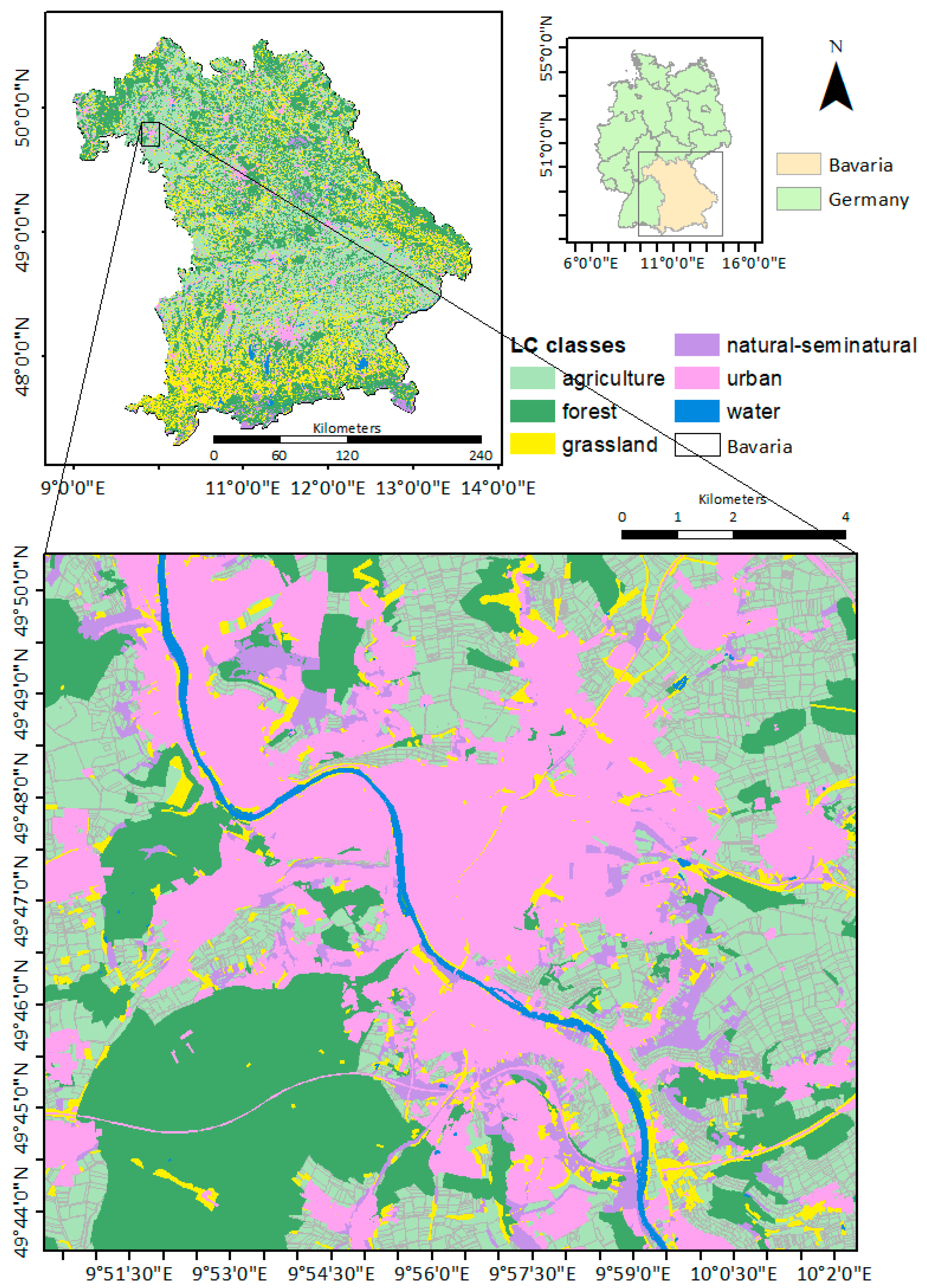
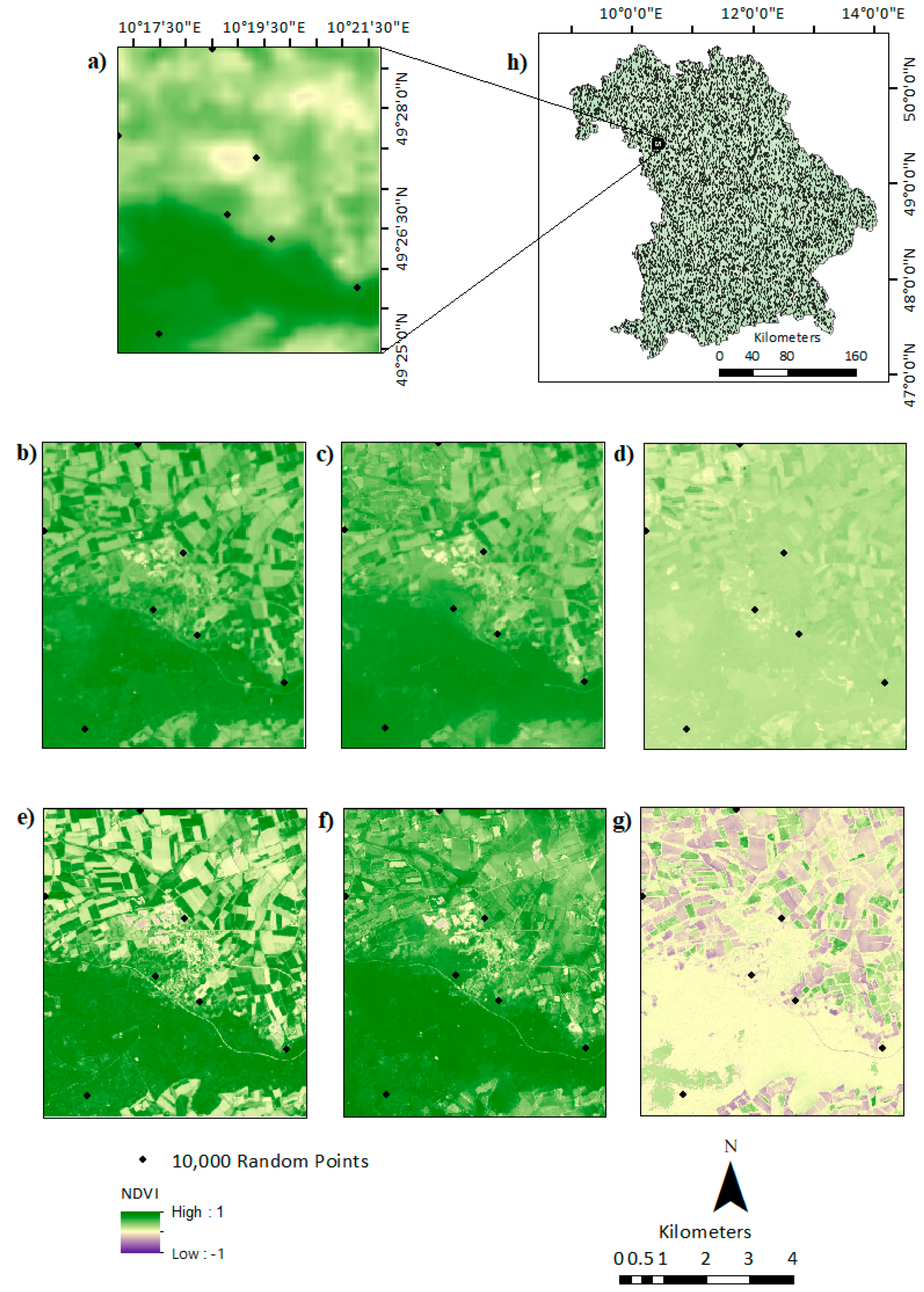
The general workflow of the study is shown in Figure 1. Different combinations of low spatial resolution (low pair) data (MOD13Q1 (16-day, 250 m), MCD43A4 (1-day, 500 m), MOD09GQ (8-day, 250 m), and MOD09Q1 (1-day, 250 m)) and high spatial resolution (high pair) data (Landsat 8 (16-day, 30 m) and Sentinel-2 (5–6-day, 10 m)) are used as an input to STARFM. The fusion process generates eight synthetic NDVI products for Bavaria in 2019. Before data fusion, the input satellite data is preprocessed by removing the clouds and shadows using quality assurance (QA) data (Figure 2). The NDVI of the raw satellite data is calculated, and then the gaps by cloud and shadow removal were filled by linear interpolation in the following steps. In the last stages of preprocessing, the input data is reprojected, resampled, and masked using the LC map of Bavaria for 2019. The correlation analysis and accuracy assessment of 8 synthetic NDVI products are done separately for every LC class (agriculture, urban, forest, grassland, water, and natural-seminatural). The high and low pair data sets are downloaded and preprocessed in Google Earth Engine (GEE), and the fusion analysis is done in R (version 4.0.3) using RStudio at the University of Wuerzburg, Germany.

2.1. Study Area

The study area of Bavaria is located between 47°N and 50.5°N, and between 9°E and 14° E, in the southeastern part of Germany (Figure 3). The topography strongly influences the region’s climate, with higher elevations in the south (northern edge of the Alps) and east (Bavarian Forest and Fichtel Mountains). The mean annual temperature ranges from −3.3 to 11 °C, but in most of the territory, the mean annual temperature ranges between 8 and 10 °C [31]. The mean annual precipitation sums range from 515 to 3184 mm, with wetter conditions in the southern part of Bavaria. In 2019, the landcover was highly dominated by forest (36.91%) and agriculture (31.67%) (based on LC map of Bavaria, 2019). The agricultural areas are mainly found in the northwest and southwest of Bavaria, while forest cover dominates towards the Alps and in the east of Bavaria. The other landcover classes like grassland, urban, natural-semi natural, and water cover, 19.16%, 8.97%, 1.84%, and 1.44%, respectively (based on LC map of Bavaria, 2019). Open grasslands and larger water areas are primarily localized in the Alpine region and Alpine foothills. Bavaria is divided into 96 counties, with Munich and Nuremberg constituting the most significant metropolitan areas.

2.2. Data

The study collected different satellite data with different spatial and temporal resolutions. A brief description of the data used in the present study with their spatial and temporal resolutions and references are shown in Table 1.

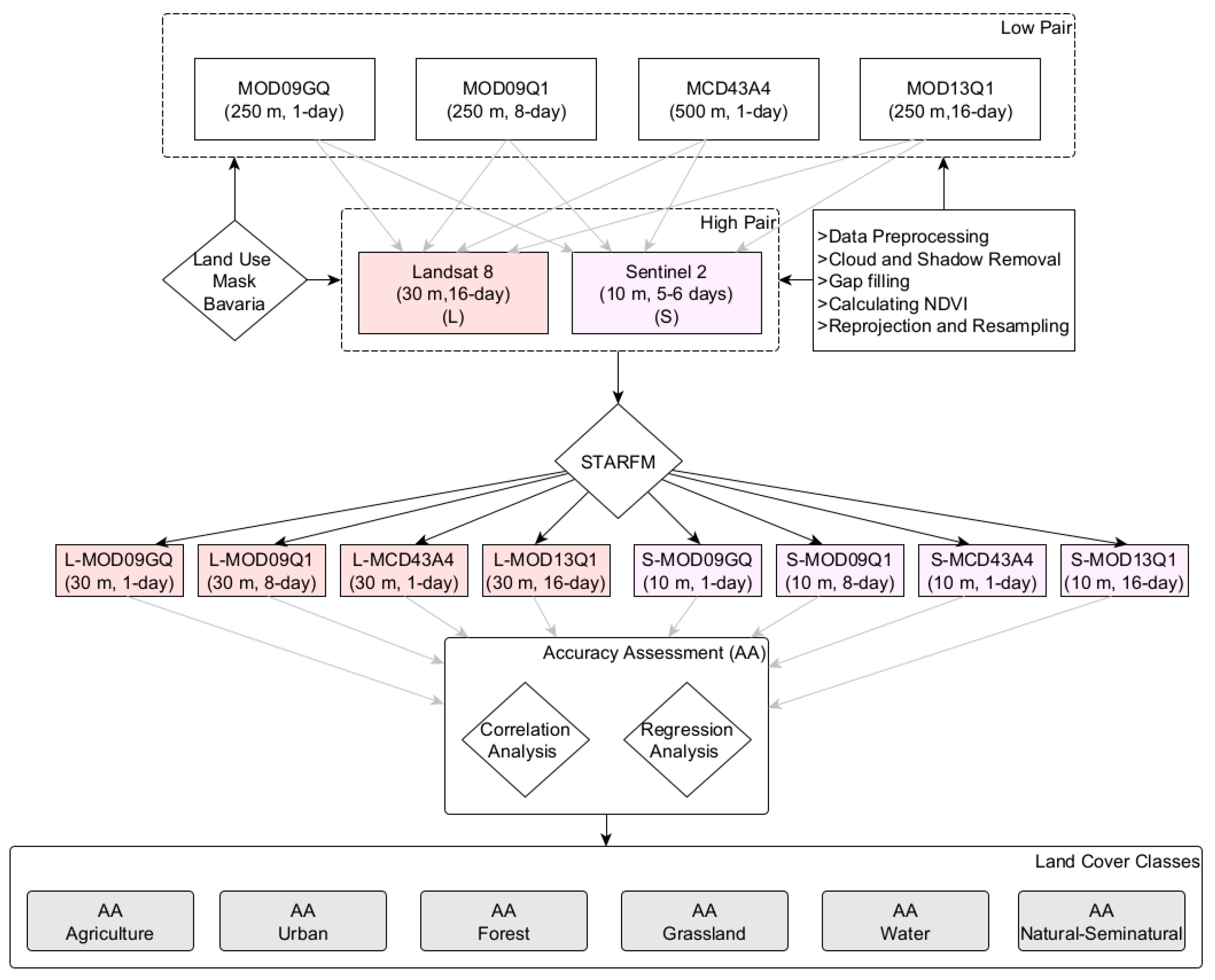
2.2.1. Satellite Data

High Spatial Resolution NDVI Products: High Pairs

For the spatio-temporal analysis, the study uses freely accessible spatially high-resolution products from Landsat 8 Land Surface Reflectance Code (LASRC) and Sentinel-2 Copernicus program. The LASRC Tier 1 has a spatial resolution of 30 m on a Universal Transverse Mercator (UTM) projection and provides seven spectral bands (coastal/aerosol, blue, green, red, near-infrared (NIR), shortwave infrared (SWIR) 1, SWIR 2). The data is atmospherically corrected using LASRC. The given quality assessment band “pixel_qa,” generated using the C function of mask (CFMask) algorithm, removes snow (using the Bit 4 of pixel_qa), clouds (Bit 5), and cloud-shadows (Bit 3) via the snow, shadow, and cloud masks. After preprocessing, the available snow-free, cloud-free, and shadow-free Landsat images were acquired in 2019 for the state of Bavaria at the following day-of-year (DOY), date respectively: 49 (18 February), 81 (22 March), 145 (25 May), 177 (26 June), 193 (12 July), 209 (28 July), 225 (13 August), 241 (29 August), and 289 (16 October) (Figure 2).
The study also uses Sentinel-2 data that allows for multi-spectral imaging with 12 spectral bands in 10–20 m spatial resolution, with global coverage and a five-day revisit frequency. The surface reflectance data of Sentinel-2 is downloaded from the Copernicus Open Access Hub and processed using the Google Earth Engine (accessed on 2 August 2021) [32]. The data was computed by sen2cor, where the cloud-free images are produced using three quality assessment (QA) bands with QA60 bitmask band containing cloud mask information. The data of Sentinel-2 is acquired at the following DOY, date respectively: 49 (18 February), 81 (22 March), 97 (07 April), 113 (23 April), 145 (25 May), 177 (26 June), 193 (12 July), 209 (28 July), 241 (29 August), 257 (14 September), 273 (30 September), 289 (16 October), and 353 (19 December) (Figure 2).

Low Spatial Resolution NDVI Products: Low Pairs

Additionally, the study uses four different MODIS NDVI products, namely MOD09Q1, MOD09GQ, MCD43A4, and MOD13Q1, with different spatial and temporal resolutions. MODIS MCD43A4 version (V) 6 Nadir Bidirectional reflectance Distribution Function (BRDF)-Adjusted Reflectance (NBAR) dataset that is produced daily using 16 days of Terra and Aqua MODIS data at 500 m spatial resolution. Both the cloud cover and the noise are removed from the quality index included in the product. The cloud gaps in the MODIS data are filled using linear interpolation.
The MOD13Q1 V6 product provides an NDVI value per pixel basis with 250 m spatial and 16-day temporal resolution. Based on the quality information (QA), pixels with the constraints were masked out. MOD13Q1 is a composed product, assigning the pixel value with the minor rules and best viewing geometry to the first date of a 16 days’ time frame. Linear interpolation of all NDVI values was performed by taking the day of acquisition (doa) science data set and the QA into account [33]. The 16-day data of MOD13Q1 is acquired at the following DOY, date respectively: 1 (1 January), 17 (17 January), 33 (02 February), 49 (18 February), 65 (06 March), 81 (22 March), 97 (07 April), 113 (23 April), 129 (09 May), 145 (25 May), 161 (10 June), 177 (26 June), 193 (12 July), 209 (28 July), 225 (13 August), 241 (29 August), 257 (14 September), 273 (30 September), 289 (16 October), 305 (01 November), 321 (17 November), 337 (03 December), and 353 (19 December).
MOD09GQ V6 surface reflectance product provides an estimate of the surface spectral reflectance as it would be measured at ground level in the absence of atmospheric scattering. It provided bands 1 (red) and 2 (NIR) at a 250 m resolution in a daily gridded L2G product in the sinusoidal projection, including quality control (QC) and five observation layers. NDVI of the product is calculated by using the available surface reflectance bands.
MOD09Q1 V6 estimated the surface reflectance of bands 1 (red) and 2 (NIR) at 250 m resolution and corrected for atmospheric conditions for 8 days’ time frame. Along with the two-reflectance bands, the quality layer removes clouds and shadows. The 8-day data of MOD09Q1 DOYs, and dates are acquired with an interval of 8 days starting from 1 (1 January) to 353 (19 December) with a total of 45 scenes.

2.2.2. LC Map of Bavaria 2019

The LC map of Bavaria is generated by combining Amtliche Topographisch-Kartographische Informationssystem (ATKIS), Integrated Administration Control System (IACS), and Corine LC (100m) at ArcGIS pro 2.2.0 (Figure 3). The ATKIS data describes the topographical objects of the landscape in vector format, generated by the official surveying system in Germany, and IACS generates all agricultural plots in European Union (EU) countries by allowing farmers to graphically indicate their agricultural areas. Combining ATKIS, IACS, and Corine LC aims to create an updated LC map of the entire Bavaria for 2019. The features of each dataset are reclassified into pre-defined land use (sub) classes, such as, agriculture (annual crops, perennial crops, and annual crop/managed grassland), forest (deciduous, coniferous, and mixed forest), grassland (managed and permanently managed grassland), urban (settlements and traffic), water, and natural-seminatural (small woody features, wetland, unmanaged grassland, and succession area). Layers with the same land use from different sources are combined into one layer. Selection of every LC class is based on the priority of data sources, for instance, agriculture: IACS > ATKIS, forest: ATKIS, grassland: IACS > ATKIS; urban: ATKIS, water: ATKIS, natural-seminatural: Corine LC > IACS > ATKIS. However, if there are conflicts among the data sources or if there are holes in the area (i.e., no information from both IACS and ATKIS), the gap is filled with Corine LC. This study uses the LC map to mask the high and low pair data fusion inputs into six LC classes before using them for the fusion process.

2.3. Method

The STARFM is used to fuse both Landsat and Sentinel-2 with four different MODIS data sets to configure the best spatial, temporal time series with high spatial and temporal resolution. Before applying the fusion algorithm, a single band of NDVI from every time step has been generated from the reflectance bands of the Landsat, Sentinel-2, and MODIS data. Before the data fusion, the MODIS daily NDVI dataset is reprojected and resampled to Landsat and Sentinel-2 imageries using bilinear interpolation. The fused model is based on the principle that low- and high-resolution products have the same NDVI values, which are biased by a constant error due to their differences in data processing, acquisition time, bandwidth, and geolocation errors. The algorithm states that if a high-low spatial resolution image pair is available on the same DOY, this constant error can be calculated for each pixel in the image. After that, these errors can be applied to the available MODIS dataset of a prediction date to obtain a prediction image with the exact spatial resolution of Landsat, or Sentinel-2 respectively. According to [10], this is done in four steps: (i) The MODIS time series is reprojected and resampled to the available corresponding high spatial resolution imagery. (ii) Next, a moving window is applied to the high spatial resolution image to identify the similar neighboring pixels. (iii) After that, the weight of Wijk is assigned to each similar neighbor. (iv) Lastly, the NDVI of the central pixel is calculated.
After obtaining the STARFM time series, the study validates the received synthetic product by dropping a single available high spatial resolution NDVI image during the fusion process and comparing both actual (the dropped high spatial resolution NDVI) and synthetic (STARFM NDVI) images of the same time zone [2]. The STARFM performs the fusion process using Equation (1) for Landsat (L) and Sentinel-2 (S):
L ( or   S ) ( x w 2 , y w 2 , t o ) = i = 1 w j = 1 w k = 1 n W ijk ( M ( x i , y i , t o ) + L ( or   S ) ( x i , y i , t k ) M ( x i , y i , t k ) ) ,
where w is the size of the moving window, L (or S) (xw/2, y w/2, to) is the central pixel of the moving window for the Landsat (Sentinel-2) image prediction at a time to, and x w/2, y w/2 is the central pixel within the moving window, the spatial weighting function Wi,j,k determines how much each neighboring pixel xi, yj in w contributes to the estimated reflectance of the central pixel. (xi, yj, to) is the MODIS reflectance at the window location (xi, yj) observed at to, while L (S) (xi, yj, tk) and M (xi, yj, tk) are the corresponding Landsat (Sentinel-2) and MODIS pixel values observed at the base date tk [10]. The n counts for the total number of input pairs of L (S) (xi, yj, tk) and M (xi, yj, tk), and each pair is supposedly acquired on the same date. The size of the moving window is taken as 1500 m by 1500 m, which is three times the size of the MODIS (MCD43A4) pixel (500 m), six times that of the MODIS (MOD13Q1, MOD09Q1, and MOD09GQ) pixel (250 m), 50 times that of the Landsat pixel (30 m) and 150 times that of the Sentinel-2 pixel [24]. The windows minimize the effect of pixel outliers and are therefore used for predicting changes using the spatially and spectrally weighted mean difference of pixels within the window area [10,20].

2.3.1. Correlations between Reference and Synthetic NDVI Time Series

The first step of the present study is a correlation analysis between STARFM NDVI and the pre-processed Landsat and Sentinel-2 images to determine when and where the synthetic NDVI product differs from the real-time satellite imagery. NDVI is one of the most widely used vegetation indices in RS and is defined as follows [34,35]:
NDVI = ρ NIR ρ Red ρ NIR + ρ Red
where ρ NIR is the reflectance in the near-infrared band and ρ Red is the reflectance in the red band. The correlation coefficient is calculated by taking the square root of Equation (3), where R is the coefficient of correlation. This process would signify the best performing location and time for regions in Bavaria on eight different synthetic output results.

2.3.2. Regression Analysis between Reference and Synthetic NDVI Time Series

The STARFM NDVI data are validated with the pre-processed, cloud and shadow-free Landsat and Sentinel-2 images acquired during the study period. From the predicted NDVI (STARFM NDVI) and observed NDVI (Landsat/Sentinel-2 NDVI), the coefficient of determination (R2) (Equation (3)) and root mean square error (RMSE) (Equation (4)) are calculated. In the last steps, the final NDVI STARFM and the pre-processed Landsat and Sentinel-2 products are masked with Bavarian LC (e.g., agriculture, forest, water, urban, grasslands, natural-seminatural), and the regression analysis between them is carried out for each LC class.
R 2 = ( (   P i   P   ) ( O i   O   ) ) 2 (   P i   P   ) ) 2 (   O i   O   ) ) 2 ,
RMSE = 1 n 1 = 1 n ( O i P i ) 2 ,
where Pi is the predicted value, Oi is the observed value, P’ is the predicted mean, O’ is the observed mean value, and n is the total number of observations. To check the significance of the fusion products, the probability value (p-value) is calculated using a Linear Regression Model (LRM) with the null hypotheses (H0) that there is no relationship between the measured and synthetic NDVI values and an H1 that the relationship exists. To perform this test, a significance level (also called alpha (α)) is set to 0.05. A p-value of less than 0.05 shows that a model is significant, and it rejects the H0 that there is no relationship.

3. Results

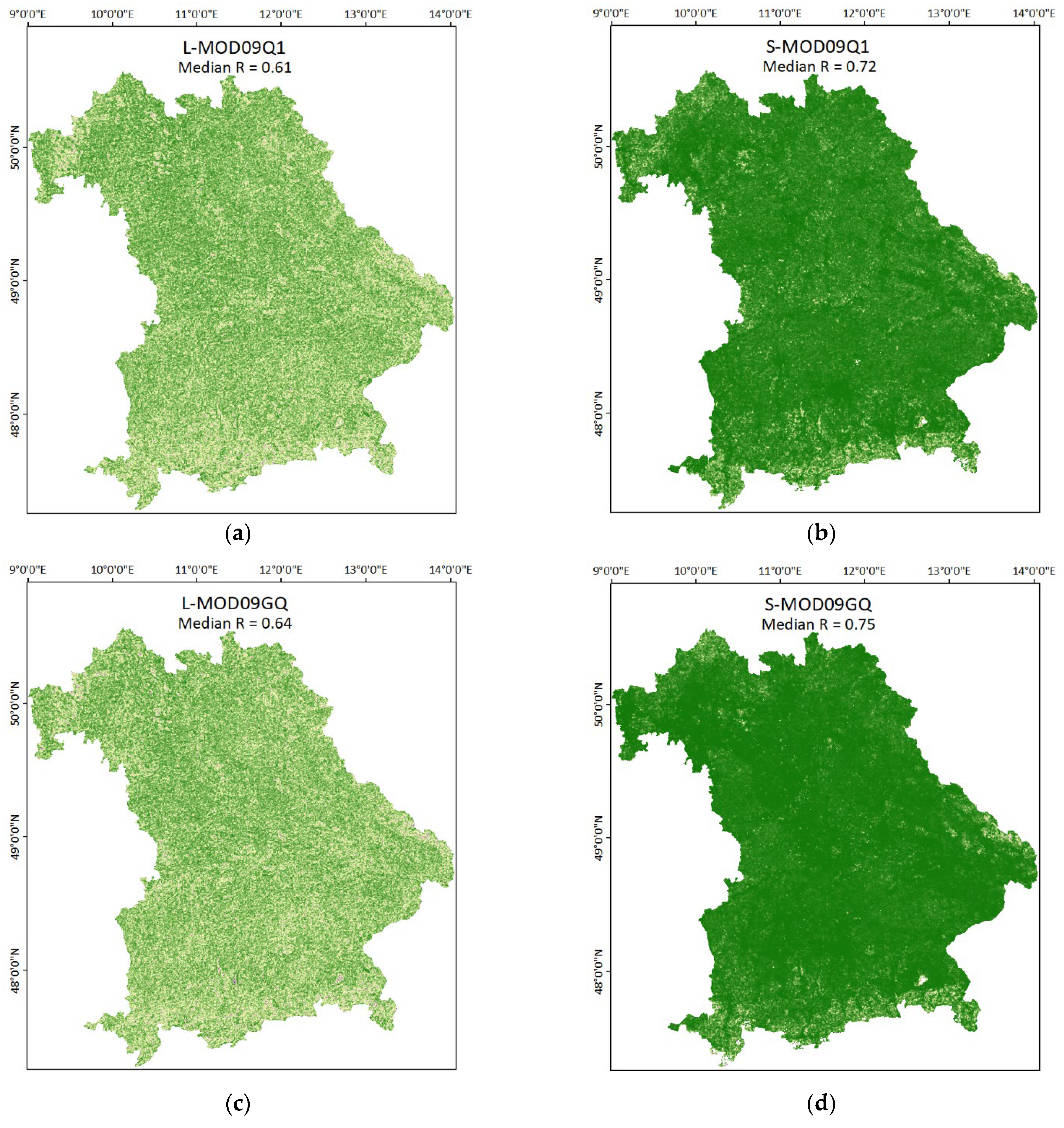
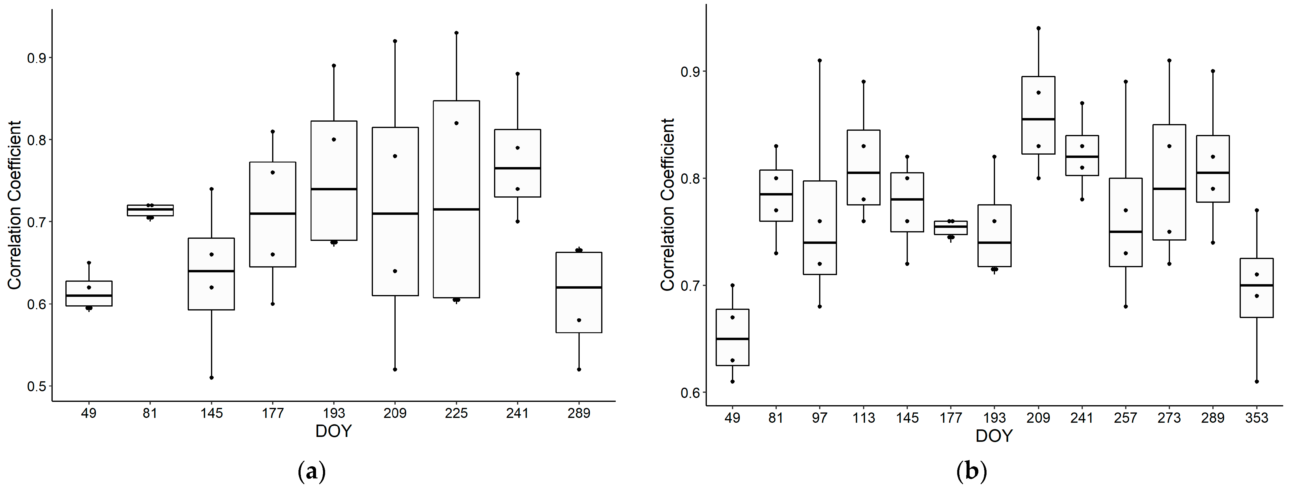
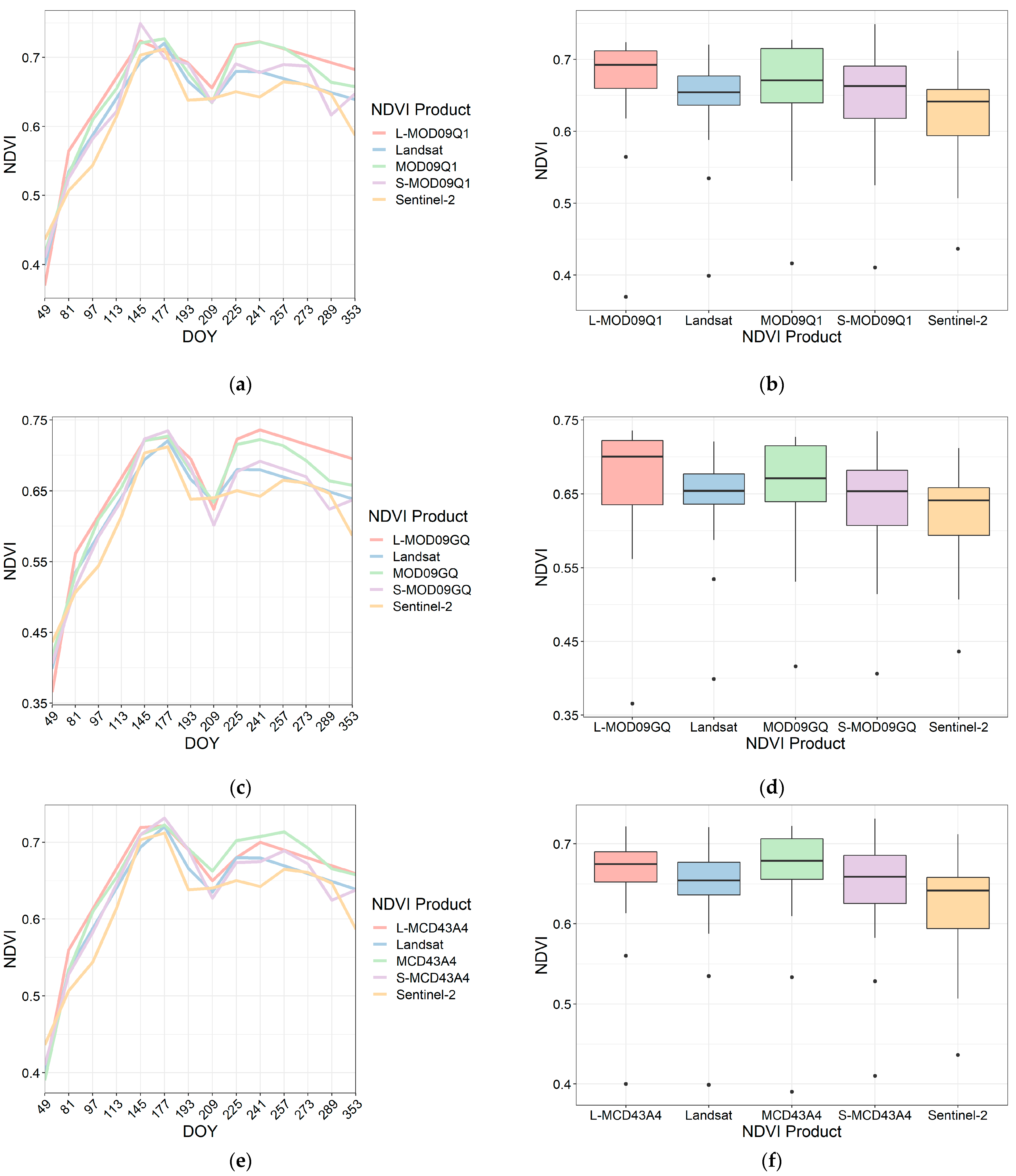
3.1. Correlations between Reference and Synthetic NDVI Time Series of Landsat and Sentinel-2

The reference and synthetic relationships show dependency on many factors, as visualized in Figure 4 by the yearly mean correlations between actual and synthetic NDVI products of Landsat and Sentinel-2 after individually fusing with multiple MODIS products. The factors show the impact of high temporal frequency and more cloud-free scenes of the high pair product on the quality of the fusion process. For example, the NDVI products L-MOD09Q1 and L-MOD09GQ result in lower positive correlation coefficients than S-MOD09Q1 and S-MOD09GQ. Almost all MODIS products show higher correlations when combined with Sentinel-2 than with Landsat, except the synthetic product L-MOD13Q1, which showed similar positive correlations as S-MOD13Q1.
Comparing the synthetic products based on their respective MODIS product used in the fusion process, L-MOD13Q1 and S-MOD13Q1 have shown the median correlation coefficient (refers to R2 in Equation (3)) of 0.81 and 0.87, respectively (Figure 4). The S-MCD43A4 positively correlated slightly better than L-MCD43A4 with a median correlation of 0.81 and 0.76, respectively. L-MOD09GQ and L-MOD09Q1 both resulted in a median of less than 0.70; however, the values of S-MOD09GQ and S-MOD09Q1 lie between 0.70 to 0.75. This considerable variation in these two products could be due to the high temporal frequency and availability of cloud-free scenes of Sentinel-2 than Landsat.
On comparing the fusion products based on the available DOYs, the DOY 209 showed the highest correlation with Landsat and Sentinel-2 synthetic products (Figure 5). For the maximum values, Sentinel-2 based fusion showed a high correlation for DOYs 49 and 289; however, for the DOYs from 183 to 241, Landsat shows higher correlation values than Sentinel-2. This suggests that the STARFM performs better for Landsat when the number of consecutive cloud-free scenes is higher.

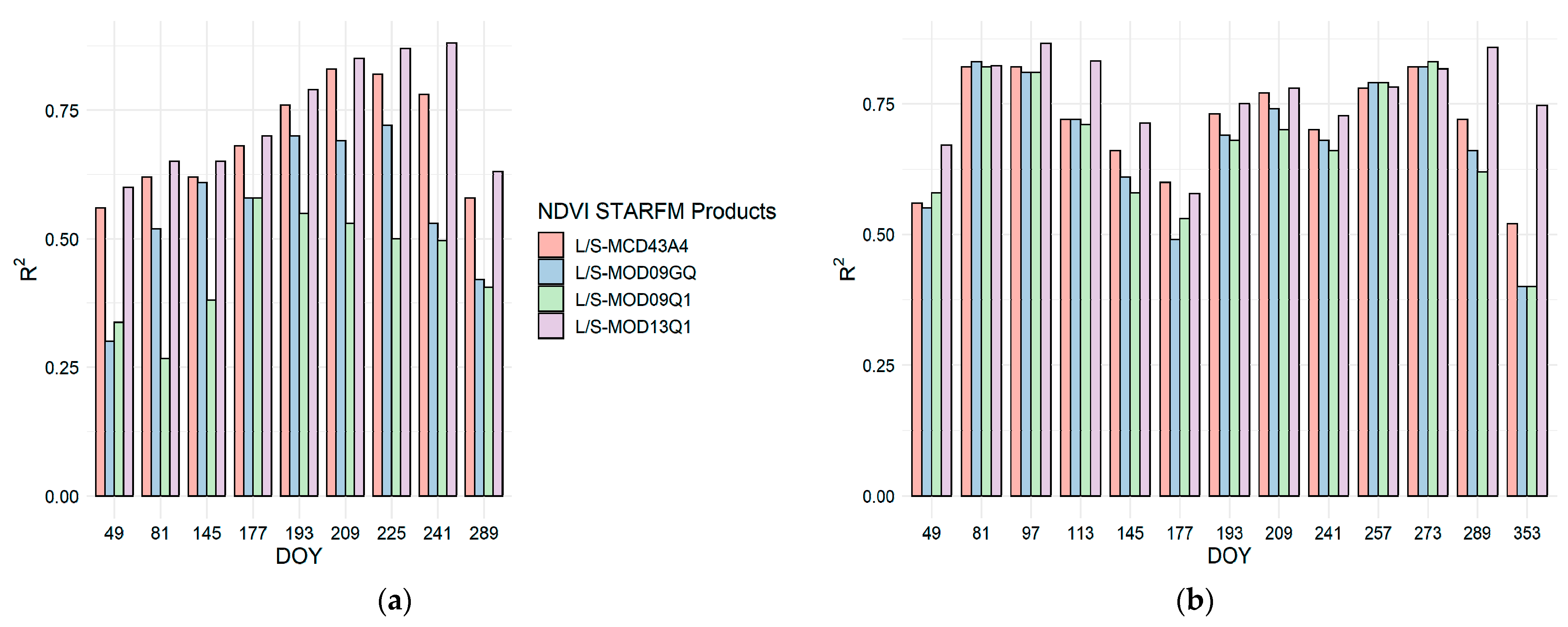
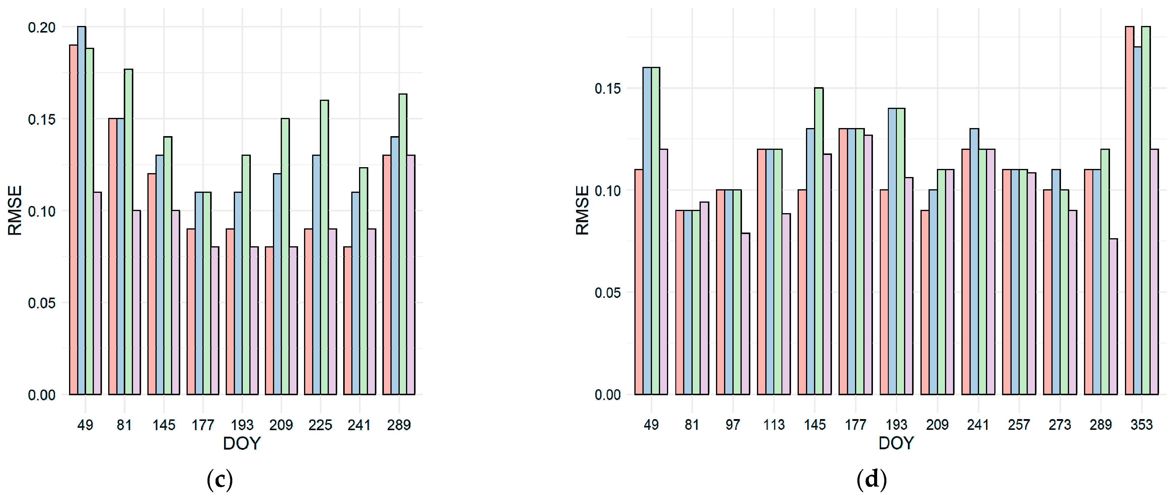
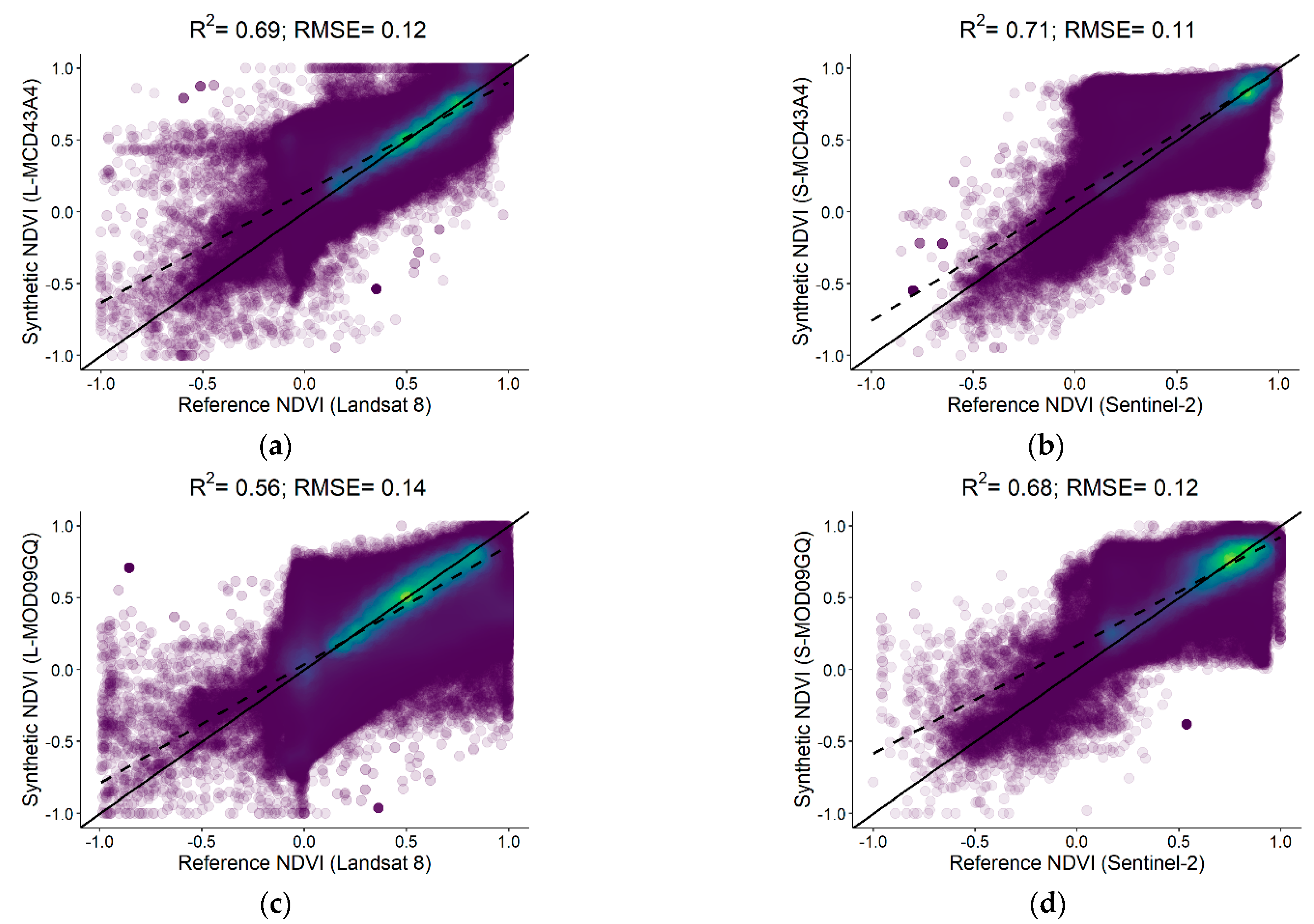
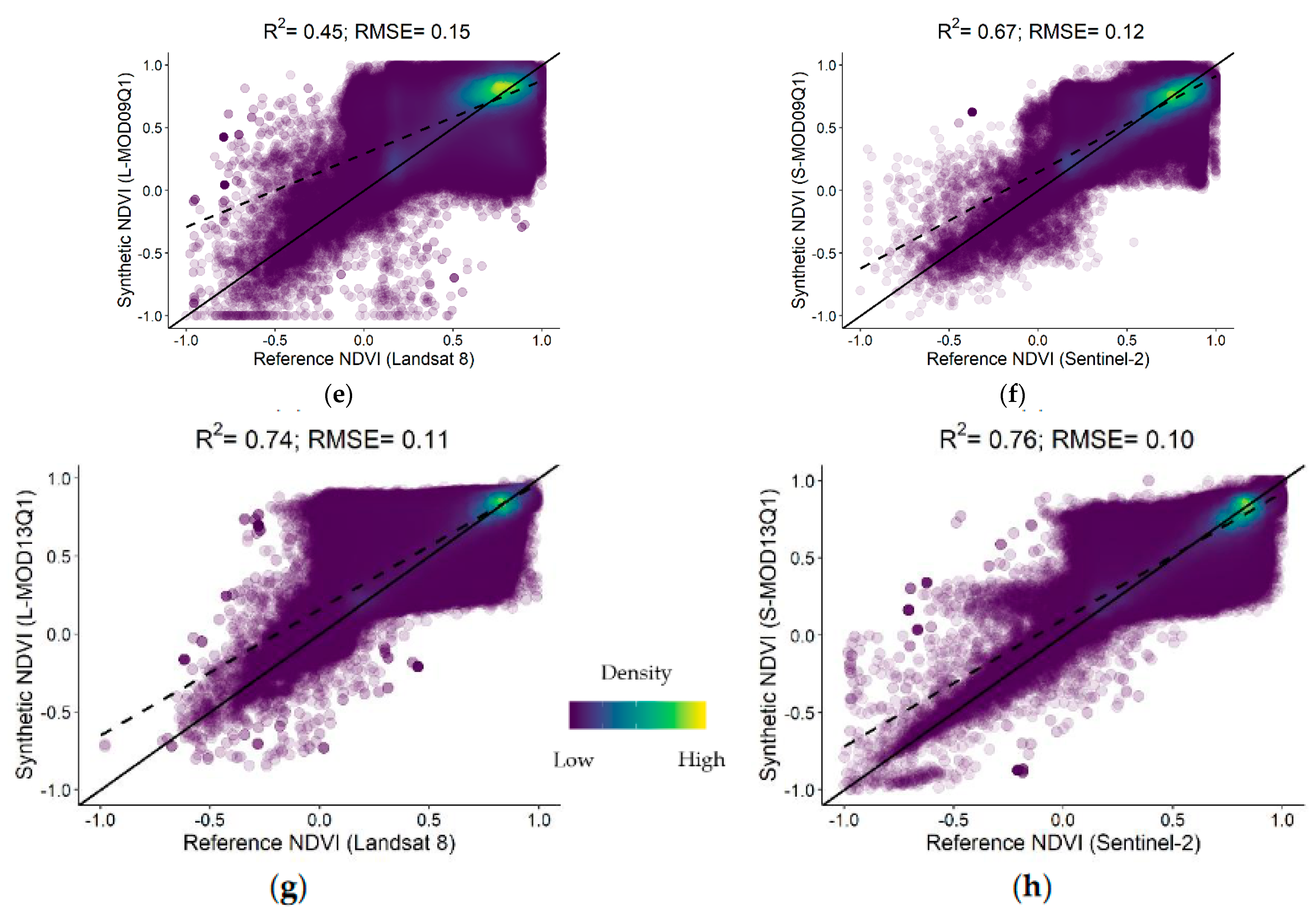
3.2. Statistical Analysis between Reference and Synthetic NDVI Time Series of Landsat and Sentinel-2

For eight different synthetic products, the STARFM performed significantly for every synthetic output (having a p-value < 0.05); this rejects the H0 of the linear regression model that there is no correlation between the reference and synthetic NDVI. After generating the scatter plots, all synthetic products’ R2, and RMSE values are analyzed. The histograms compare different MODIS products when fused with Landsat and Sentinel-2 on a DOY-basis (Figure 6). Both L-MOD13Q1 and S-MOD13Q1 result in high R2 (0.74 and 0.76) and low RMSE (<0.11) compared to L/S-MCD43A4, L/S-MOD09GQ, and L/S-MOD09Q1. For L-MCD43A4, L-MOD09GQ, and L-MOD09Q1, the R2 (0.69, 0.56, 0.45) and RMSE (0.12, 0.14, 0.15) values vary in an order of higher accuracy. However, for Sentinel-2, this trend is more accurate and homogenous with R2 and RMSE of 0.71 and 0.11 (S-MCD43A4), 0.68 and 0.12 (S-MOD09GQ), 0.67 and 0.12 (S-MOD09Q1).
Compared on a DOY-basis, the synthetic L-MOD13Q1 and S-MCD13Q1 show the top edge in almost all the DOYs. The L-MOD13Q1 and L-MCD43A4 result in closer R2 and RMSE; however, S-MCD43A4, S-MOD09GQ, S-MOD09Q1 result in similar accuracies. The vast contrast in the accuracies of Landsat and Sentinel-2 is seen in DOYs 49 and 289 with the synthetic product of L/S-MOD13Q1 with an R2 of 0.62, 0.76, and RMSE of 0.12, 0.10, respectively. On comparing the accuracies of Landsat and Sentinel-2 for all fused pairs, synthetic products generated with Sentinel-2 resulted more accurately and precisely than Landsat, respectively (Figure 7).

3.3. Statistical Analysis between Reference and Synthetic NDVI Time Series of Landsat and Sentinel-2 Based on Land Use Classes

Table 2 and Table 3 show the accuracy and precision of eight different synthetic products categorized on LC classes such as agriculture, forest, grassland, seminatural-natural, urban, and water at different DOYs. The urban and water classes resulted in the higher R2 and lower RMSE with Landsat and Sentinel-2 than other land use classes. Both classes within S-MCD43A4, S-MOD09GQ, and S-MOD09Q1 resulted in higher mean R2 values more than 0.75 and lower mean RMSE of ~0.08 (urban) and ~0.12 (water), respectively. Both with L-MOD13Q1 and S-MOD13Q1, the class of agriculture resulted with high R2 (0.62, 0.68) and low RMSE (0.11, 0.13) compared to other STARFM products. In addition, the mean R2 and RMSE for agriculture in S-MCD43A4, S-MOD09GQ, and S-MOD09Q1 are nearly similar with values 0.66 and 0.14, respectively. The forest class in L-MOD13Q1 showed the higher accuracy (R2 = 0.60, RMSE = 0.05) than S-MOD13Q1 (R2 = 0.52, RMSE = 0.09). MOD09GQ and MOD09Q1 performed better with Sentinel-2 than Landsat. Even though the water class resulted in high R2 with both high-resolution products, the RMSE of the same is quite high (>0.10) with all MODIS products. On the contrary, the forest class resulted in very low RMSE (~0.08) despite having rather low R2 values.

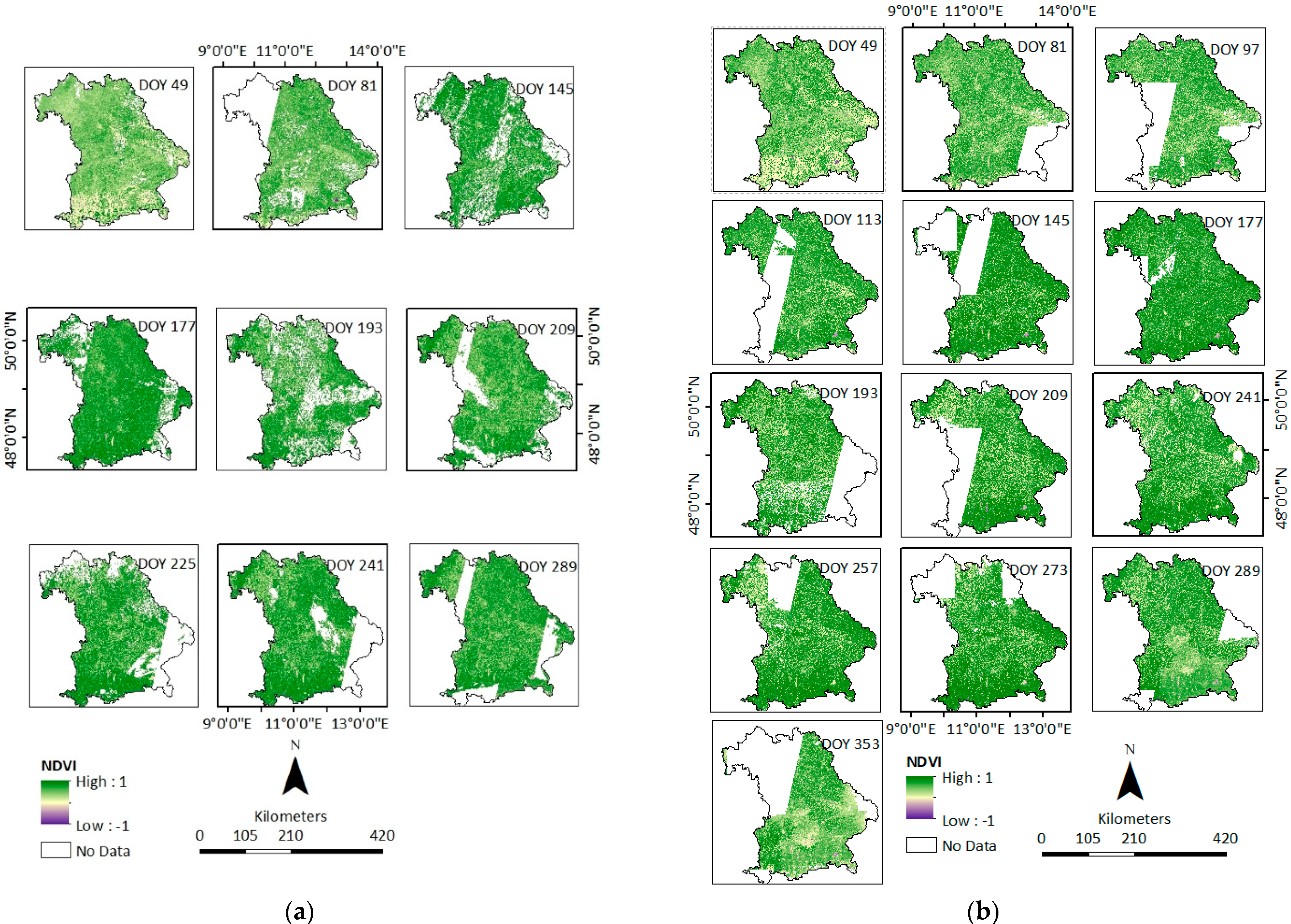
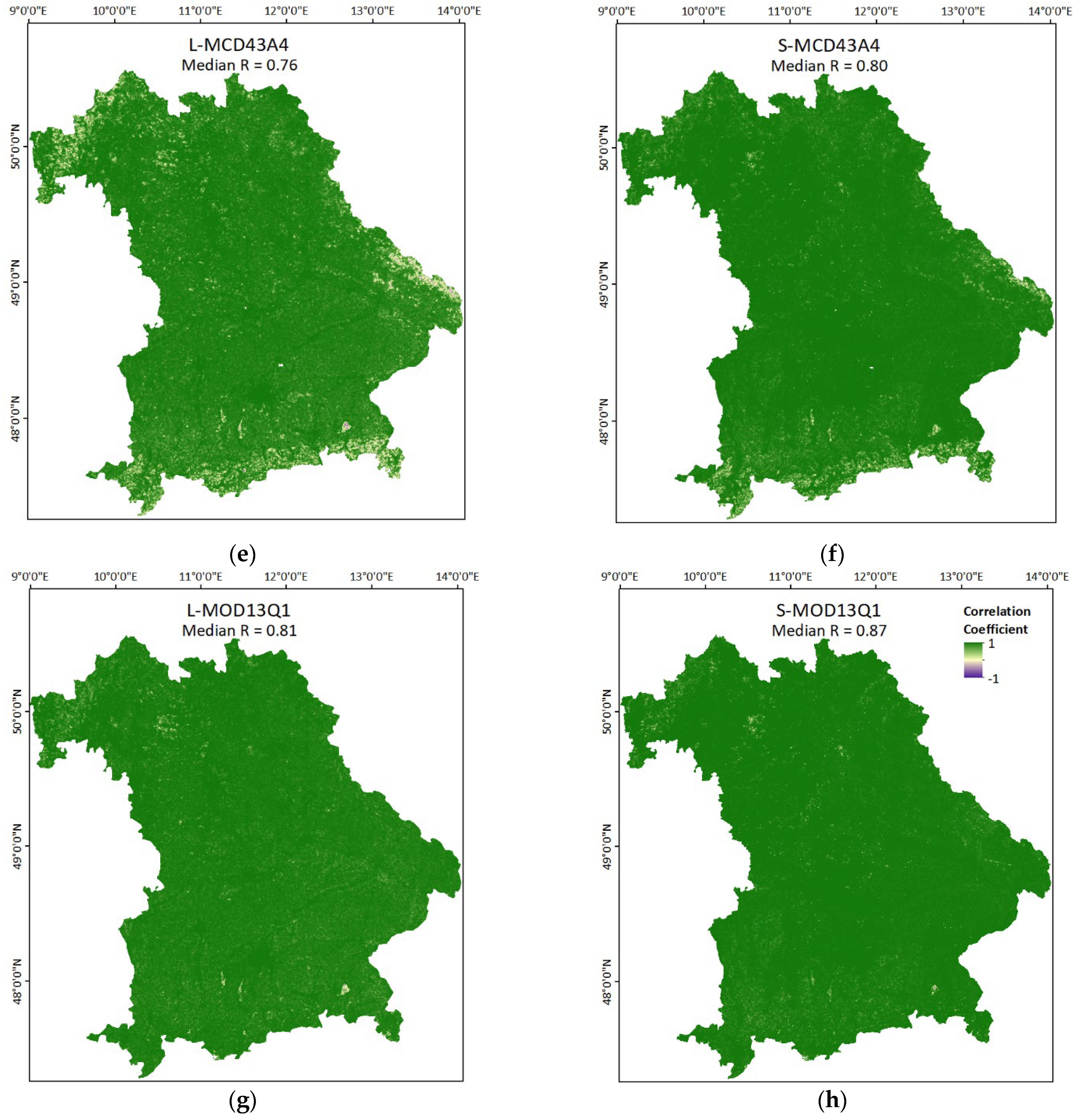
3.4. Visualization of Resulted Synthetic Products Obtained from Different MODIS Imageries

The spatial visualization of the products MOD13Q1, Landsat, L-MOD13Q1, Landsat minus L-MOD13Q1, Sentinel-2, S-MOD13Q1, Sentinel-2 minus S-MOD13Q1 at DOY 193 is shown in Figure 8a–g, respectively. Figure 8d,g show the slight overestimation and underestimation of NDVI values with the synthetic product (L/S-MOD13Q1) is subtracted from its respective reference high-resolution products (Landsat or Sentinel-2). Figure 8h shows the spatial location of 10,000 random points that compares eight synthetic products with their respective low pair (MODIS) and high pair (Landsat or Sentinel-2) products by considering the mean values at different DOYs (Figure 9). Figure 9a–h shows the line plot comparison of eight synthetic products along with their interquartile comparison of NDVI values.
Both L-MOD13Q1 and S-MOD13Q1 show a slight overestimation and underestimation of NDVI values compared to the reference Landsat and Sentinel-2 NDVI values at different DOYs. The median NDVI values of L-MOD13Q1 and S-MOD12Q1 lie close to their respective high pair product. However, the difference in median values of synthetic products from their high pair products increases from L/S-MCD43A4, L/S-MOD09GQ, and L/S-MOD09Q1, respectively. The mean NDVI values (Figure 9a,c) and median (Figure 9b,d) of L-MOD09GQ and L-MOD09Q1 lie close to their low pair MOD09GQ and MOD09Q1 products than the Landsat. However, the products S-MOD09GQ and S-MOD09Q1 lie closer to Sentinel-2. This might be the reason that the accuracies of S-MOD09GQ and S-MOD09Q1 resulted higher than that of L-MOD09GQ and L-MOD09Q1.

4. Discussion

4.1. Quality Assessment of Data Fusion

The study investigates the capability of the STARFM [10] over the Bavarian state of Germany to generate the synthetic NDVI time series of 2019 by testing different high (Landsat (L) (16-day, 30 m) and Sentinel-2 (S) (10 m, 5–6 day)) and low (MOD13Q1 (16-day, 250 m), MCD43A4 (1-day, 500 m), MOD09GQ (1-day, 250 m), and MOD09Q1 (8-day, 250 m)) spatial resolution products. NDVI is considered the most effective and widely acknowledged vegetation index among other vegetation indices. Various studies with spatiotemporal data fusion have used NDVI as their primary input for different applications such as phenology analysis [5,30,36,37], yield and drought monitoring [2,38,39,40], forest mapping [20,41], and biophysical parameter estimation [40,42,43,44]. However, many spatiotemporal fusion algorithms are based on reflectance fusion, which needs more computation power than the NDVI fusion.
The study uses the strategy “index-then-blend” (IB), which generates the NDVI from both high pair and low pair images before they are blended for the data fusion [26]. On the contrary, many studies first blend the reflectance of the individual MODIS and Landsat data sets and then generate the NDVI using the “blend-then-index” (BI) approach [37,45]. Ref. [26] has conducted a theoretical and experimental analysis that states if the predicted NDVI values are lower than the input Landsat values, IB performs better and vice versa. Among 10,000 randomly selected points in the entire Bavaria, some predicted higher NDVI values, and the remaining plots predicted lower; therefore, both BI and IB errors are expected to be small [26]. Additionally, the IB approach has less computation cost than BI, as it blends only one band: the NDVI. Therefore, the present study decided to perform the IB approach’s fusion analysis.
Many studies have started using the combined use of Landsat and Sentinel-2 for RS applications [46,47,48,49]. The 16-day temporal resolution of Landsat is not fine enough to monitor a variety of landscape changes. The recent launch of new satellite missions such as Landsat 9, Sentinel-2A, or Sentinel-2B can ensure a much higher temporal sampling rate that could grab an image every 2–5 or 8–16 days when sensor bands are combined, similarly concerning the spectral information. Even though the NASA Harmonized Landsat and Sentinel-2 (HLS) project produces temporal dense reflectance product at 30 m, the cloud and shadow gaps in both datasets would still exist [50,51]. Moreover, the limit of HLS to some selected test sites and the wasted spatial information at 10 m must still be borne in mind. However, the STARFM algorithm is convenient to be applied on any test site without losing the spatial resolution of respective high pair data.
In this study, four MODIS products with different spatial and temporal resolutions are fused with Landsat and Sentinel-2 to test the best suitable pair for the NDVI time series of Bavaria in 2019. An advantage of combining MODIS with high spatial resolution products is to generate synthetic results, which exceed the physical limitations of Landsat/Sentinel-2 and contain more information than the original input images [52,53]. For example, Sentinel-2 and MODIS can be fused to generate a dataset with high spatial resolution (10 m) with daily/8-day temporal resolution. In the past, many studies have used the simple temporal filtering methods to fill the cloud and shadow generated gaps in satellite inputs by interpreting the intensities at a certain pixel position over time [54,55,56]. For example, the simplicity of the linear interpolation method could still capture changes over time if the changes follow a linear trend. However, to examine the real-time trends in different RS applications, the data fusion methods resulted more prominently in filling those gaps with a real-time multi-sensor information, which can reduce the uncertainties in the synthetic data [56,57]. This study investigates factors responsible for the accuracy assessment of the eight synthetic products generated by STARFM. These factors state that the high temporal frequency and more cloud-free scenes of the respective high pair (Landsat/Sentinel-2) would impact the overall accuracy of the fusion process [2]. Due to the low temporal frequency of Landsat data (16 days) and higher cloud cover, the synthetic product obtained using different MODIS outputs is not as accurate as Sentinel-2 (5–6 days) [3,4]. For example, the availability of 13 cloud-free scenes of Sentinel-2 in 2019 result in higher accuracy of S-MOD09GQ (R2 = 0.68, RMSE = 0.12) and S-MOD09Q1 (R2 = 0.65, RMSE = 0.13), as compared to L-MOD09GQ (R2 = 0.56, RMSE = 0.13) and L-MOD09Q1 (R2 = 0.45, RMSE = 0.15), with nine partially available cloud-free scenes of Landsat. Similarly, the spatial correlation of the obtained synthetic product is higher when Sentinel-2 data is used as an input with MODIS products than Landsat, respectively. However, Sentinel-2 shows higher accuracy, its spatial resolution of 10 m consumes more storage and increases the computing load.
Among the MODIS products, MCD13Q1 and MCD43A4 showed higher accuracy and higher positive spatial correlation with both Landsat and Sentinel-2. However, with a frequency of one day, MCD43A4 with 500 m spatial resolution makes the data storage heavier with more run-time than MCD13Q1 with 250 m spatial and 16 days revisit. Moreover, MCD13Q1 is a high-quality product employed in more than 1700 peer-reviewed research articles (Google Scholar), and its fewer cloud contaminated pixels resulted in higher accuracy in data fusion [58,59,60]. In addition, comparing the better product between MCD13Q1 and MCD43A4 also depends on the requirement. The required product will be selected accordingly if the need is to generate a time series with a daily or 16-day frequency. On the other hand, L/S-MOD09GQ and L/S-MOD09Q1 result in higher accuracy with Sentinel-2 than Landsat. This justifies that high pair product plays a significant role in the accuracy assessment of any synthetic product. Moreover, L-MOD09GQ and L-MOD09Q1 showed a weak spatial correlation with their reference Landsat images. Contrarily, the opposite was true for S-MOD09GQ and S-MOD09Q1. The obtained R2 and RMSE of these synthetic products obtained through the STARFM are comparable to those obtained by other studies [10,23,61]. Comparing the accuracy, storage, and processing time required between L/S-MOD09GQ and L/S-MOD09Q1, the former is not only more accurate, but it also needs less storage and lower computation power due to its 8-day temporal resolution. However, high cloud coverage and gaps put them on the least accurate NDVI synthetic products list.

4.2. Quality Assessment of Data Fusion based on Different Land Use Classes

To evaluate the suitability of the STARFM for homogenous landscapes, this study individually runs the algorithm for six different land use classes: agriculture, forest, urban, water, grassland, and seminatural-natural. The spatial correlation of other classes greatly influences the used high pair product. The data fusion results of the study indicate that the STARFM can successfully fuse MODIS with both Landsat and Sentinel-2 [4,62]. On average, synthetic time series with Sentinel-2 showed more positive correlations than Landsat. However, comparing accuracy assessments based on different low pair products used, each class varied differently. Almost every synthetic product is accurate and precise for the water and urban classes with a high to low variation from L/S-MOD13Q1, L/S-MCD43A4 L/S-MOD09GQ, and L/S-MOD09Q1. This might be because the values of these classes remain similar throughout the year; however, for agriculture, synthetic products obtained using Sentinel-2 resulted in higher accuracy than Landsat. This could be because the chances of mixed pixels are lesser for agricultural fields with lower spatial resolution. Exceptionally, L-MOD13Q1 resulted in similar accuracy and preciseness as S-MOD13Q1 for the agriculture class. This justifies that both products are suitable for the application of agricultural monitoring. The only difference separating them is their computation power and data storage. S-MOD13Q1 needs high processing power and time with high storage capacity due to its 10-m spatial resolution. Similarly, comparing L-MOD13Q1 and S-MOD13Q1 for the forest class, the former resulted in higher accuracy than the latter. Therefore, this proves that both L-MOD13Q1 and S-MOD13Q1 are suitable for agricultural and forest monitoring; however, L-MOD13Q1 has the upper hand due to its fast and easy processing with less storage requirement. Besides that, the present study compares the synthetic NDVI products generated from the STARFM, where NDVI is mostly considered as a suitable parameter for the applications of forest, grassland, and agriculture [35,39]. However, this study recommends to include other indices, such as Normalized Difference Built-up Index (NDBI) and Normalized Difference Water Index (NDWI) for the applications of urban and water, respectively [63,64]. Moreover, many studies have suggested more improvements in the respective fusion algorithm [3,17,20].

4.3. Visualization of the NDVI Synthetic Products

In the visualization process, 10,000 random points were randomly chosen to extract the NDVI values in Bavaria, and their mean values at different DOYs were used to compare the eight synthetic products with their respective low pair (MODIS) and high pair (Landsat or Sentinel-2) products. For products L-MOD13Q1, L-MCD43A4, S-MOD13Q1, S-MCD43A4, S-MOD09GQ, and S MOD09Q1, the mean values obtained lie close to their respective high-resolution product. Therefore, the accuracy of these products is higher. The closer the synthetic product with its separate spatial resolution, the higher the accuracy. However, for the products L-MOD09GQ and L MOD09Q1, the obtained NDVI values lie close to their MODIS data; this could be due to the quality of their respective MODIS products and Landsat images.

5. Conclusions

The present study compares the performance of eight NDVI synthetic products generated using the STARFM for the entire state of Bavaria in 2019. The output of the fusion model is obtained by inputting two high pairs (Landsat (L) (16-day, 30 m) and Sentinel-2 (S) (10 m, 5–6 day)) and four low pairs (MOD13Q1 (16-day, 250 m), MCD43A4 (1-day, 500 m), MOD09GQ (1-day, 250 m), and MOD09Q1 (8-day, 250 m)). Due to the suitability of STARFM for homogenous landscapes, the study compares the eight different outputs 1) on Bavarian level, and 2) on six different land use classes level, namely agriculture, forest, grassland, urban, water, and natural-seminatural.
The study found that the higher revisit frequency and more cloud and shadow-free scenes of the respective high pair product can impact the synthetic product’s spatial correlation and accuracy. For example, the availability of 13 cloud-free scenes of Sentinel-2 (5–6 days) in 2019, result in higher accuracy of S-MOD09GQ (R2 = 0.68, RMSE = 0.12) and S-MOD09Q1 (R2 = 0.65, RMSE = 0.12), as compared to L-MOD09GQ (R2 = 0.56, RMSE = 0.14) and L-MOD09Q1 (R2 = 0.45, RMSE = 0.15), with 9 partially available cloud-free scenes of Landsat (16 days). Conclusively, it also states that the synthetic products obtained using Sentinel-2 are more accurate than products obtained using Landsat. Therefore, Sentinel-2 could be used as an input high pair product for the STARFM. The study also compares the synthetic NDVI products based on their respective low pair input used in the blending process. This resulted that L/S-MOD13Q1 (R2 = 0.74/0.76, RMSE = 0.11/0.10) showed higher spatial correlation than L/S-MCD43A4 (R2 = 0.69/0.71, RMSE = 0.12/0.11), L/S-MOD98GQ, L/S-MOD09Q1. This concludes that the MOD13Q1 is the best suitable low pair product because of its higher quality. Moreover, due to its temporal resolution of 16 days, the fusion process takes less computation time to produce the synthetic RS product, even at a large scale.
On comparing the synthetic NDVI products on different land use classes, the urban and water classes resulted in the higher R2 (>0.75) and lower RMSE (0.08, and 0.12, respectively) with both Landsat and Sentinel-2 than the other land use classes. For agricultural and forest classes, both L-MOD13Q1 and S-MOD13Q1 showed higher accuracy than the other products. With bothL-MOD13Q1 and S-MOD13Q1, the class of agriculture resulted with an R2 of 0.62, and 0.68 and RMSE of 0.11, and 0.13, and the forest class with an R2 of 0.60, and 0.52 and RMSE of 0.05, and 0.09, respectively. Conclusively, both L-MOD13Q1 and S-MOD13Q1 are suitable for agricultural and forest monitoring; however, the spatial resolution of 30 m and low storage capacity makes L-MOD13Q1 more prominent and faster than that of S-MOD13Q1 with the 10-m spatial resolution. From an application perspective, both products (L-MOD13Q1 and S-MOD13Q1) could be further tested for the RS application of crop yield estimation.

Author Contributions

Conceptualization, M.S.D., T.D. and T.U.; Methodology, M.S.D.; Software, M.S.D.; Validation, M.S.D.; Formal Analysis, M.S.D. and T.U.; Investigation, M.S.D.; Resources, M.S.D., T.D., C.K.-F., J.Z., I.S.-D. and T.U.; Data Curation, M.S.D., C.K.-F. and J.Z.; Writing—original draft preparation, M.S.D.; Writing—review and editing, M.S.D. and T.U.; Visualization, M.S.D., and T.U.; Supervision, T.U.; Project Administration, C.K.-F. and T.D.; Funding Acquisition, I.S.-D. All authors have read and agreed to the published version of the manuscript.

Funding

This research received no external funding. This publication is supported by the Open Access Publication Fund of the University of Wuerzburg. The research is a part of the LandKlif project funded by the Bavarian Ministry of Science and the Arts via the Bavarian Climate Research Network (bayklif: https://www.bayklif.de/) (accessed on 1 March 2019).

Data Availability Statement

Publicly available satellite datasets were analyzed in this study. This data can be found here: [MODIS SR] LP DAAC. 2019. MOD13Q1 v006; https://lpdaac.usgs.gov/products/mod13q1v006/ (access on 10 September 2019); (MODIS SR) LP DAAC. 2021. MCD43A4 v006; https://lpdaac.usgs.gov/products/mcd43a4v006/ (access on 10 July 2021); (MODIS SR) LP DAAC. 2021. MOD09GQ v006; https://lpdaac.usgs.gov/products/mod09gqv006/ (access on 18 July 2021); (MODIS SR) LP DAAC. 2021. MOD09Q1 v006; https://lpdaac.usgs.gov/products/mod09q1v006/ (access on 18 July 2021); (Landsat 8 SR) Landsat 8; https://www.usgs.gov/ (access on 12 April 2019); (Landsat 8 SR) Sentinel-2; https://sentinels.copernicus.eu/web/sentinel/ (access on 2 August 2021).

Acknowledgments

The authors thankfully express gratitude to the National Aeronautics and Space Administration (NASA) Land Processed Distributed Active Archive Center (LP DAAC) for MODIS; U.S. Geological Survey (USGS) Earth Resources Observation and Science (EROS) Center for Landsat; The Copernicus Sentinel-2 mission for the Sentinel-2 data; Professorship of Ecological Services, University of Bayreuth, for the updated Land Cover Map of Bavaria 2019; Jie Zhang and Sarah Redlich, both Department of Animal Ecology and Tropical Biology, University of Wuerzburg, developed the initial concept and methodology for the Land Cover Map of Bavaria; together with Melissa Versluis, Rebekka Riebl, Maria Hänsel, Bhumika Uniyal, Thomas Koellner (all Professorship of Ecological Services, University of Bayreuth) this concept and methodology were further developed; Melissa Versluis (Professorship of Ecological Services, University of Bayreuth) has created the Land Cover Map of 2019 based on the concluding methodology for whole Bavaria; we acknowledge the data providers for the base layers ATKIS (Bayerische Vermessungsverwaltung), IACS (Bayerisches Staatsministerium für Ernährung, Landwirtschaft und Forsten) and Corine LC (European Environment Agency).; Simon Sebold for providing all technical and computational help during the complete fusion processing of Landsat/Sentinel-2 and MODIS; Department of Remote Sensing, University of Wuerzburg, for providing all necessary resources and support; Google Earth Engine platform for faster downloading and preprocessing the large data sets of Bavaria; The Comprehensive R Archive Network (CRAN) for running the STARFM, and validating and visualizing the data outputs using R packages such as raster, rgdal, ggplot2, ggtools, and xlsx; ArcGIS 10.8 and ArcGIS pro 2.2.0 maintained by Environmental Systems Research Institute (Esri) for generating maps and Bavarian Land Cover Map of 2019; and the Bavarian Ministry for Science and the Arts via the Bavarian Climate Research Network (bayklif) for funding.

Conflicts of Interest

The authors declare no conflict of interest.

References

  1. Dubovik, O.; Schuster, G.L.; Xu, F.; Hu, Y.; Bösch, H.; Landgraf, J.; Li, Z. Grand Challenges in Satellite Remote Sensing. Front. Remote Sens. 2021, 2, 619818. [Google Scholar] [CrossRef]
  2. Dhillon, M.S.; Dahms, T.; Kuebert-Flock, C.; Borg, E.; Conrad, C.; Ullmann, T. Modelling Crop Biomass from Synthetic Remote Sensing Time Series: Example for the DEMMIN Test Site, Germany. Remote Sens. 2020, 12, 1819. [Google Scholar] [CrossRef]
  3. Roy, D.P.; Ju, J.; Lewis, P.; Schaaf, C.; Gao, F.; Hansen, M.; Lindquist, E. Multi-temporal MODIS–Landsat data fusion for relative radiometric normalization, gap filling, and prediction of Landsat data. Remote Sens. Environ. 2008, 112, 3112–3130. [Google Scholar] [CrossRef]
  4. Gevaert, C.M.; García-Haro, F.J. A comparison of STARFM and an unmixing-based algorithm for Landsat and MODIS data fusion. Remote Sens. Environ. 2015, 156, 34–44. [Google Scholar] [CrossRef]
  5. Bhandari, S.; Phinn, S.; Gill, T. Preparing Landsat Image Time Series (LITS) for Monitoring Changes in Vegetation Phenology in Queensland, Australia. Remote Sens. 2012, 4, 1856–1886. [Google Scholar] [CrossRef] [Green Version]
  6. Arai, E.; Shimabukuro, Y.E.; Pereira, G.; Vijaykumar, N.L. A Multi-Resolution Multi-Temporal Technique for Detecting and Mapping Deforestation in the Brazilian Amazon Rainforest. Remote Sens. 2011, 3, 1943–1956. [Google Scholar] [CrossRef] [Green Version]
  7. Dariane, A.B.; Khoramian, A.; Santi, E. Investigating spatiotemporal snow cover variability via cloud-free MODIS snow cover product in Central Alborz Region. Remote Sens. Environ. 2017, 202, 152–165. [Google Scholar] [CrossRef]
  8. Dong, C.; Menzel, L. Improving the accuracy of MODIS 8-day snow products with in situ temperature and precipitation data. J. Hydrol. 2016, 534, 466–477. [Google Scholar] [CrossRef]
  9. Parajka, J.; Bloschl, G. Spatio-temporal combination of MODIS images—Potential for snow cover mapping. Water Resour. Res. 2008, 44. [Google Scholar] [CrossRef]
  10. Gao, F.; Masek, J.; Schwaller, M.; Hall, F. On the blending of the Landsat and MODIS surface reflectance: Predicting daily Landsat surface reflectance. IEEE Trans. Geosci. Remote Sens. 2006, 44, 2207–2218. [Google Scholar] [CrossRef]
  11. Xie, D.; Zhang, J.; Zhu, X.; Pan, Y.; Liu, H.; Yuan, Z.; Yun, Y. An Improved STARFM with Help of an Unmixing-Based Method to Generate High Spatial and Temporal Resolution Remote Sensing Data in Complex Heterogeneous Regions. Sensors 2016, 16, 207. [Google Scholar] [CrossRef] [PubMed] [Green Version]
  12. Cui, J.; Zhang, X.; Luo, M. Combining Linear Pixel Unmixing and STARFM for Spatiotemporal Fusion of Gaofen-1 Wide Field of View Imagery and MODIS Imagery. Remote Sens. 2018, 10, 1047. [Google Scholar] [CrossRef] [Green Version]
  13. Lee, M.H.; Cheon, E.J.; Eo, Y.D. Cloud Detection and Restoration of Landsat-8 using STARFM. Korean J. Remote Sens. 2019, 35, 861–871. [Google Scholar] [CrossRef]
  14. Zhu, L.; Radeloff, V.C.; Ives, A.R. Improving the mapping of crop types in the Midwestern U.S. by fusing Landsat and MODIS satellite data. Int. J. Appl. Earth Obs. Geoinf. 2017, 58, 1–11. [Google Scholar] [CrossRef]
  15. Zhang, J. Multi-source remote sensing data fusion: Status and trends. Int. J. Image Data Fusion 2010, 1, 5–24. [Google Scholar] [CrossRef] [Green Version]
  16. Belgiu, M.; Stein, A. Spatiotemporal Image Fusion in Remote Sensing. Remote Sens. 2019, 11, 818. [Google Scholar] [CrossRef] [Green Version]
  17. Zhu, X.; Chen, J.; Gao, F.; Chen, X.; Masek, J.G. An enhanced spatial and temporal adaptive reflectance fusion model for complex heterogeneous regions. Remote Sens. Environ. 2010, 114, 2610–2623. [Google Scholar] [CrossRef]
  18. Olexa, E.M.; Lawrence, R.L. Performance and effects of land cover type on synthetic surface reflectance data and NDVI estimates for assessment and monitoring of semi-arid rangeland. Int. J. Appl. Earth Obs. Geoinf. 2014, 30, 30–41. [Google Scholar] [CrossRef]
  19. Wu, M.; Niu, Z.; Wang, C.; Wu, C.; Wang, L. Use of MODIS and Landsat time series data to generate high-resolution temporal synthetic Landsat data using a spatial and temporal reflectance fusion model. J. Appl. Remote Sens. 2012, 6, 63507. [Google Scholar] [CrossRef]
  20. Hilker, T.; Wulder, M.A.; Coops, N.C.; Linke, J.; McDermid, G.; Masek, J.G.; Gao, F.; White, J.C. A new data fusion model for high spatial- and temporal-resolution mapping of forest disturbance based on Landsat and MODIS. Remote Sens. Environ. 2009, 113, 1613–1627. [Google Scholar] [CrossRef]
  21. Huang, B.; Song, H. Spatiotemporal Reflectance Fusion via Sparse Representation. IEEE Trans. Geosci. Remote Sens. 2012, 50, 3707–3716. [Google Scholar] [CrossRef]
  22. Luo, Y.; Guan, K.; Peng, J. STAIR: A generic and fully-automated method to fuse multiple sources of optical satellite data to generate a high-resolution, daily and cloud-/gap-free surface reflectance product. Remote Sens. Environ. 2018, 214, 87–99. [Google Scholar] [CrossRef]
  23. Emelyanova, I.V.; McVicar, T.R.; Van Niel, T.G.; Li, L.T.; van Dijk, A.I.J.M. Assessing the accuracy of blending Landsat–MODIS surface reflectances in two landscapes with contrasting spatial and temporal dynamics: A framework for algorithm selection. Remote Sens. Environ. 2013, 133, 193–209. [Google Scholar] [CrossRef]
  24. Zhu, X.; Cai, F.; Tian, J.; Williams, T.K.-A. Spatiotemporal Fusion of Multisource Remote Sensing Data: Literature Survey, Taxonomy, Principles, Applications, and Future Directions. Remote Sens. 2018, 10, 527. [Google Scholar] [CrossRef] [Green Version]
  25. Htitiou, A.; Boudhar, A.; Benabdelouahab, T. Deep Learning-Based Spatiotemporal Fusion Approach for Producing High-Resolution NDVI Time-Series Datasets. Can. J. Remote Sens. 2021, 47, 182–197. [Google Scholar] [CrossRef]
  26. Chen, X.; Liu, M.; Zhu, X.; Chen, J.; Zhong, Y.; Cao, X. “Blend-then-Index” or “Index-then-Blend”: A Theoretical Analysis for Generating High-resolution NDVI Time Series by STARFM. Photogramm. Eng. Remote Sens. 2018, 84, 65–73. [Google Scholar] [CrossRef]
  27. Jarihani, A.A.; McVicar, T.; Van Niel, T.G.; Emelyanova, I.; Callow, J.; Johansen, K. Blending Landsat and MODIS Data to Generate Multispectral Indices: A Comparison of “Index-then-Blend” and “Blend-then-Index” Approaches. Remote Sens. 2014, 6, 9213–9238. [Google Scholar] [CrossRef] [Green Version]
  28. Rao, Y.; Zhu, X.; Chen, J.; Wang, J. An Improved Method for Producing High Spatial-Resolution NDVI Time Series Datasets with Multi-Temporal MODIS NDVI Data and Landsat TM/ETM+ Images. Remote Sens. 2015, 7, 7865–7891. [Google Scholar] [CrossRef] [Green Version]
  29. Liao, C.; Wang, J.; Pritchard, I.; Liu, J.; Shang, J. A Spatio-Temporal Data Fusion Model for Generating NDVI Time Series in Heterogeneous Regions. Remote Sens. 2017, 9, 1125. [Google Scholar] [CrossRef] [Green Version]
  30. Qiu, Y.; Zhou, J.; Chen, J.; Chen, X. Spatiotemporal fusion method to simultaneously generate full-length normalized difference vegetation index time series (SSFIT). Int. J. Appl. Earth Obs. Geoinf. 2021, 100, 102333. [Google Scholar] [CrossRef]
  31. Kloos, S.; Yuan, Y.; Castelli, M.; Menzel, A. Agricultural Drought Detection with MODIS Based Vegetation Health Indices in Southeast Germany. Remote Sens. 2021, 13, 3907. [Google Scholar] [CrossRef]
  32. Gorelick, N.; Hancher, M.; Dixon, M.; Ilyushchenko, S.; Thau, D.; Moore, R. Google Earth Engine: Planetary-scale geospatial analysis for everyone. Remote Sens. Environ. 2017, 202, 18–27. [Google Scholar] [CrossRef]
  33. Kuebert, C. Fernerkundung für das Phänologiemonitoring: Optimierung und Analyse des Ergrünungsbeginns mittels MODIS-Zeitreihen für Deutschland; University of Wuerzburg: Würzburg, Germany, 2018. [Google Scholar]
  34. Rouse, J.W.; Haas, R.H.; Schell, J.A.; Deering, D.W.; Harlan, J.C. Monitoring the Vernal Advancement and Retrogradation (Green Wave Effect) of Natural Vegetation; NASA/GSFC Type III Final Report; Texas A&M University: College Station, TX, USA, 1974. [Google Scholar]
  35. Tucker, C.J. Red and photographic infrared linear combinations for monitoring vegetation. Remote Sens. Environ. 1979, 8, 127–150. [Google Scholar] [CrossRef] [Green Version]
  36. Hwang, T.; Song, C.; Bolstad, P.V.; Band, L.E. Downscaling real-time vegetation dynamics by fusing multi-temporal MODIS and Landsat NDVI in topographically complex terrain. Remote Sens. Environ. 2011, 115, 2499–2512. [Google Scholar] [CrossRef]
  37. Walker, J.J.; De Beurs, K.M.; Wynne, R.H.; Gao, F. Evaluation of Landsat and MODIS data fusion products for analysis of dryland forest phenology. Remote Sens. Environ. 2012, 117, 381–393. [Google Scholar] [CrossRef]
  38. Htitiou, A.; Boudhar, A.; Lebrini, Y.; Hadria, R.; Lionboui, H.; Elmansouri, L.; Tychon, B.; Benabdelouahab, T. The Performance of Random Forest Classification Based on Phenological Metrics Derived from Sentinel-2 and Landsat 8 to Map Crop Cover in an Irrigated Semi-arid Region. Remote Sens. Earth Syst. Sci. 2019, 2, 208–224. [Google Scholar] [CrossRef]
  39. Benabdelouahab, T.; Lebrini, Y.; Boudhar, A.; Hadria, R.; Htitiou, A.; Lionboui, H. Monitoring spatial variability and trends of wheat grain yield over the main cereal regions in Morocco: A remote-based tool for planning and adjusting policies. Geocarto Int. 2019, 36, 2303–2322. [Google Scholar] [CrossRef]
  40. Lebrini, Y.; Boudhar, A.; Htitiou, A.; Hadria, R.; Lionboui, H.; Bounoua, L.; Benabdelouahab, T. Remote monitoring of agricultural systems using NDVI time series and machine learning methods: A tool for an adaptive agricultural policy. Arab. J. Geosci. 2020, 13, 1–14. [Google Scholar] [CrossRef]
  41. Xin, Q.; Olofsson, P.; Zhu, Z.; Tan, B.; Woodcock, C.E. Toward near real-time monitoring of forest disturbance by fusion of MODIS and Landsat data. Remote Sens. Environ. 2013, 135, 234–247. [Google Scholar] [CrossRef]
  42. Anderson, M.C.; Kustas, W.P.; Norman, J.M.; Hain, C.R.; Mecikalski, J.R.; Schultz, L.; González-Dugo, M.P.; Cammalleri, C.; D’Urso, G.; Pimstein, A.; et al. Mapping daily evapotranspiration at field to continental scales using geostationary and polar orbiting satellite imagery. Hydrol. Earth Syst. Sci. 2011, 15, 223–239. [Google Scholar] [CrossRef] [Green Version]
  43. Gao, F.; Anderson, M.C.; Kustas, W.P.; Wang, Y. Simple method for retrieving leaf area index from Landsat using MODIS leaf area index products as reference. J. Appl. Remote Sens. 2012, 6, 063554. [Google Scholar] [CrossRef]
  44. Singh, D. Generation and evaluation of gross primary productivity using Landsat data through blending with MODIS data. Int. J. Appl. Earth Obs. Geoinf. 2011, 13, 59–69. [Google Scholar] [CrossRef]
  45. Dong, T.; Liu, J.; Qian, B.; Zhao, T.; Jing, Q.; Geng, X.; Wang, J.; Huffman, T.; Shang, J. Estimating winter wheat biomass by assimilating leaf area index derived from fusion of Landsat-8 and MODIS data. Int. J. Appl. Earth Obs. Geoinf. 2016, 49, 63–74. [Google Scholar] [CrossRef]
  46. Quintano, C.; Fernández-Manso, A.; Fernández-Manso, O. Combination of Landsat and Sentinel-2 MSI data for initial assessing of burn severity. Int. J. Appl. Earth Obs. Geoinf. 2018, 64, 221–225. [Google Scholar] [CrossRef]
  47. Pahlevan, N.; Chittimalli, S.K.; Balasubramanian, S.V.; Vellucci, V. Sentinel-2/Landsat-8 product consistency and implications for monitoring aquatic systems. Remote Sens. Environ. 2019, 220, 19–29. [Google Scholar] [CrossRef]
  48. Moon, M.; Richardson, A.D.; Friedl, M.A. Multiscale assessment of land surface phenology from harmonized Landsat 8 and Sentinel-2, PlanetScope, and PhenoCam imagery. Remote Sens. Environ. 2021, 266, 112716. [Google Scholar] [CrossRef]
  49. Zhang, Y.; Ling, F.; Wang, X.; Foody, G.M.; Boyd, D.S.; Li, X.; Du, Y.; Atkinson, P.M. Tracking small-scale tropical forest disturbances: Fusing the Landsat and Sentinel-2 data record. Remote Sens. Environ. 2021, 261, 112470. [Google Scholar] [CrossRef]
  50. Claverie, M.; Ju, J.; Masek, J.G.; Dungan, J.L.; Vermote, E.F.; Roger, J.-C.; Skakun, S.V.; Justice, C. The Harmonized Landsat and Sentinel-2 surface reflectance data set. Remote Sens. Environ. 2018, 219, 145–161. [Google Scholar] [CrossRef]
  51. Bolton, D.K.; Gray, J.; Melaas, E.K.; Moon, M.; Eklundh, L.; Friedl, M.A. Continental-scale land surface phenology from harmonized Landsat 8 and Sentinel-2 imagery. Remote Sens. Environ. 2020, 240, 111685. [Google Scholar] [CrossRef]
  52. Lunetta, R.S.; Lyon, J.G.; Guindon, B.; Elvidge, C.D. North American landscape characterization dataset development and data fusion issues. Photogramm. Eng. Remote Sens. 1998, 64, 821–828. [Google Scholar]
  53. Pohl, C.; van Genderen, J. Multisensor image fusion in remote sensing: Concepts, methods and applications. Int. J. Remote Sens. 1998, 19, 823–854. [Google Scholar] [CrossRef] [Green Version]
  54. Gao, F.; Morisette, J.T.; Wolfe, R.E.; Ederer, G.; Pedelty, J.; Masuoka, E.; Myneni, R.; Tan, B.; Nightingale, J. An Algorithm to Produce Temporally and Spatially Continuous MODIS-LAI Time Series. IEEE Geosci. Remote Sens. Lett. 2008, 5, 60–64. [Google Scholar] [CrossRef]
  55. Borak, J.S.; Jasiński, M.F. Effective interpolation of incomplete satellite-derived leaf-area index time series for the continental United States. Agric. For. Meteorol. 2009, 149, 320–332. [Google Scholar] [CrossRef] [Green Version]
  56. Kandasamy, S.; Baret, F.; Verger, A.; Neveux, P.; Weiss, M. A comparison of methods for smoothing and gap filling time series of remote sensing observations—Application to MODIS LAI products. Biogeosciences 2013, 10, 4055–4071. [Google Scholar] [CrossRef] [Green Version]
  57. Verger, A.; Baret, F.; Weiss, M. A multisensor fusion approach to improve LAI time series. Remote Sens. Environ. 2011, 115, 2460–2470. [Google Scholar] [CrossRef] [Green Version]
  58. Robinson, N.P.; Allred, B.W.; Jones, M.O.; Moreno, A.; Kimball, J.S.; Naugle, D.E.; Erickson, T.A.; Richardson, A.D. A Dynamic Landsat Derived Normalized Difference Vegetation Index (NDVI) Product for the Conterminous United States. Remote Sens. 2017, 9, 863. [Google Scholar] [CrossRef] [Green Version]
  59. Didan, K.; Munoz, A.B.; Solano, R.; Huete, A. MODIS Vegetation Index User’s Guide (MOD13 Series); Vegetation Index and Phenology Lab, University of Arizona: Tucson, AZ, USA, 2015. [Google Scholar]
  60. Solano, R.; Didan, K.; Jacobson, A.; Huete, A. MODIS Vegetation Index User’s Guide (MOD13 Series); Terrestrial Biophysics and Remote Sensing Lab, University of Arizona: Tucson, AZ, USA, 2010. [Google Scholar]
  61. Chen, B.; Ge, Q.; Fu, D.; Yu, G.; Sun, X.; Wang, S.; Wang, H. A data-model fusion approach for upscaling gross ecosystem productivity to the landscape scale based on remote sensing and flux footprint modelling. Biogeosciences 2010, 7, 2943–2958. [Google Scholar] [CrossRef] [Green Version]
  62. Thorsten, D.; Christopher, C.; Babu, D.K.; Marco, S.; Erik, B. Derivation of biophysical parameters from fused remote sensing data. In Proceedings of the 2017 IEEE International Geoscience and Remote Sensing Symposium (IGARSS), Fort Worth, TX, USA, 23–28 July 2017; pp. 4374–4377. [Google Scholar] [CrossRef]
  63. Gao, B.-C. NDWI—A normalized difference water index for remote sensing of vegetation liquid water from space. Remote Sens. Environ. 1996, 58, 257–266. [Google Scholar] [CrossRef]
  64. Zha, Y.; Gao, J.; Ni, S. Use of normalized difference built-up index in automatically mapping urban areas from TM imagery. Int. J. Remote Sens. 2003, 24, 583–594. [Google Scholar] [CrossRef]
Figure 1. Flowchart of data used and processed to generate the synthetic NDVI time series using STARFM; STARFM = Spatial and Temporal Adaptive Reflectance Fusion Model; NDVI = Normalized Difference Vegetation Index; L-MOD09GQ = Landsat-MOD09GQ; L-MOD09Q1 = Landsat-MOD09Q1; L-MCD43A4 = Landsat-MCD43A4; L-MOD13Q1 = Landsat-MOD13Q1; S-MOD09GQ = Sentinel-2-MOD09GQ; S-MOD09Q1 = Sentinel-2-MOD09Q1; S-MCD43A4 = Sentinel-2-MCD43A4; S-MOD13Q1 = Sentinel-2-MOD13Q1; AA = Accuracy Assessment.
Remotesensing 14 00677 g001
Figure 2. The cloud-free scenes are available for (a) Landsat and (b) Sentinel-2. Nine cloud-free scenes were collected for the Landsat data, and thirteen were collected for the Sentinel-2 data. The maps show the NDVI values from -1 to 1 for the entire Bavaria during 2019.
Remotesensing 14 00677 g002
Figure 3. The LC map of Bavaria is obtained by combining multiple inputs of Landcover maps such as Amtliche Topographisch-Kartographische Informationssystem (ATKIS), Integrated Administration Control System (IACS) Corine LC, into one map. Agriculture (peach green) dominates mainly in the northwest and southeast of Bavaria, while forest and grassland classes (dark green and yellow, respectively) dominate in the northeast and south. The enlargement shows the urban area of the city Würzburg.
Remotesensing 14 00677 g003
Figure 4. The average spatial correlations between the reference Landsat and Sentinel-2 NDVI with synthetic (a) L-MOD09Q1, (b) S-MOD09Q1, (c) L-MOD98GQ, (d) S-MOD09GQ, (e) L-MCD43A4, (f) S-MCD43A4 (g) L-MOD13Q1, and (h) S-MOD13Q1, NDVI time series for 2019 respectively. The average correlation is calculated by taking the mean of dropped scenes used for calculating the accuracy assessment of the eight synthetic NDVI products. The legend of the spatial correlations (High: 1 (Green) to Low: −1 (Purple)) is provided at the top right of figure (h). The median correlation coefficient (R) is given at the top of each figure. The correlation coefficient refers to R2 (see Equation (3)).
Remotesensing 14 00677 g004aRemotesensing 14 00677 g004b
Figure 5. The day of the year (DOY) based comparison of correlation coefficients between synthetic NDVI time series and the reference NDVI values obtained from (a) Landsat and (b) Sentinel-2 with different MODIS products. The correlation coefficient refers to R2 (see Equation (3)).
Remotesensing 14 00677 g005
Figure 6. The statistical comparison shows R2 and RMSE values of different NDVI STARFM products obtained using (a,c) Landsat (L) and (b,d) Sentinel-2 (S) with varying products of MODIS, respectively. Different colors show the R2 and RMSE values with four different MODIS products: MCD43A4 (orange), MOD09GQ (blue), MOD09Q1 (green), and MOD13Q1 (purple).
Remotesensing 14 00677 g006aRemotesensing 14 00677 g006b
Figure 7. The scatter plots compare the accuracies of reference Landsat and Sentinel-2 products with synthetic (a) L-MCD43A4, (b) S-MCD43A4, (c) L-MOD98GQ, (d) S-MOD09GQ, (e) L-MOD09Q1, (f) S-MOD09Q1, (g) L-MOD13Q1, and (h) S-MOD13Q1 products, respectively. The values of the statistical parameters, such as R2 and RMSE are displayed at the top of each plot. Every plot contains a solid 1:1 line that is used to visualize the correlation of pixels between the reference and synthetic NDVI values.
Remotesensing 14 00677 g007aRemotesensing 14 00677 g007b
Figure 8. Image-wise comparison of STARFM and real-time NDVI values from (a) MOD13Q1, (b) Landsat, (c) L-MOD13Q1, (d) Landsat minus L-MOD13Q1 (difference) (e) Sentinel-2, (f) S-MOD13Q1, and (g) Sentinel-2 minus S-MOD13Q1 (difference), on DOY 193 (12th July 2019). The figure (h) shows the spatial location of 10,000 random points in Bavaria used to draw line and bar plots in Figure 9 for comparing the mean NDVI values on DOYs basis for the eight different synthetic NDVI products.
Remotesensing 14 00677 g008
Figure 9. The line and bar plots show the DOY-based and inter-quartile-range based comparison of STARFM generated NDVI values with their respective high-resolution input (Landsat (L) or Sentinel-2 (S)) and low-resolution input (a,b) MOD09Q1 (c,d) MOD09GQ, (e,f) MCD43A4, (g,h) MOD13Q1 respectively. The comparison is based on the mean values extracted for 10,000 random points (whose spatial location is shown in Figure 8h) taken for entire Bavaria.
Remotesensing 14 00677 g009aRemotesensing 14 00677 g009b
Table 1. A summary of the collected datasets. The satellite data used are Sentinel-2, Landsat 8, and Moderate Resolution Imaging Spectroradiometer (MODIS) MOD09Q1, MOD09GQ, MCD43A4, MOD13Q1; the Land Cover (LC) data is based covers six land use classes of Bavaria: agriculture, forest, urban, water, natural-semi natural, and grassland.
DataProduct NameResolution Spatial-TemporalReferences
Satellite dataSentinelSentinel-210 m 5–6 dayswww.corpenicus.eu (accessed on 21 June 2021)
LandsatLandsat 830 m 16 dayswww.usgs.gov (accessed on 21 June 2021)
MODISMOD09GQ250 m 1 day www.lpdaac.usgs.gov (accessed on 21 June 2021)
MOD09Q1250 m 8 dayswww.lpdaac.usgs.gov (accessed on 21 June 2021)
MCD43A4500 m 1 daywww.lpdaac.usgs.gov (accessed on 21 June 2021)
MOD13Q1250 m 16 dayswww.lpdaac.usgs.gov (accessed on 21 June 2021)
Vector
data
Land Cover (LC)LC Map of Bavaria2019www.landklif.biozentrum.uni-wuerzburg.de (accessed on 21 June 2021)
Table 2. The DOY-based statistical analysis (R2 and mean RMSE) between the synthetic NDVI (for four different MODIS products) and reference Landsat (L) NDVI in Bavaria for every LC class such as agriculture (31.67%), urban (8.97%), water (1.44%), forest (35.91%), seminatural-natural (1.84%) and grassland (19.16%), in 2019. The percentage represents the number of pixels in each LC class from the total number of pixels (n = 7,83,48,322). A legend table of R2 values are shown at top right of the table. The mean RMSE values are shown in white color.
NDVI ProductLC ClassDOY
4981145177193209225241289Mean R2Mean RMSE
L-MOD13Q1Agriculture0.410.490.660.650.620.790.810.640.480.620.11R2
Urban0.350.460.670.810.850.850.850.860.710.710.070.00–0.25
Water0.440.550.640.720.790.710.740.830.740.680.130.26–0.50
Forest0.490.530.600.460.670.690.720.690.500.600.050.51–0.75
Seminatural-natural0.590.640.720.640.810.810.810.810.350.690.070.76–1.00
Grassland0.300.350.350.450.660.680.680.580.500.510.11
L-MCD43A4Agriculture0.210.450.460.620.640.740.740.610.480.550.11
Urban0.140.180.620.770.860.810.850.810.790.650.07
Water0.480.500.670.590.790.740.740.740.790.670.13
Forest0.450.360.310.400.640.560.500.450.450.460.06
Seminatural-natural0.140.320.580.480.760.710.770.710.640.570.07
Grassland0.280.180.130.340.640.670.640.530.320.410.11
L-MOD09GQAgriculture0.180.220.460.260.590.610.640.580.360.430.13
Urban0.120.170.560.550.690.610.670.740.720.540.10
Water0.380.480.590.550.640.620.550.690.710.580.18
Forest0.450.370.220.170.320.270.230.310.140.280.09
Seminatural-natural0.200.460.610.560.590.590.670.490.480.520.10
Grassland0.220.150.140.250.520.520.520.460.250.340.12
L-MOD09Q1Agriculture0.240.230.380.320.450.560.410.530.300.380.15
Urban0.140.160.500.520.450.520.440.640.670.450.13
Water0.420.410.590.460.490.410.450.690.670.510.21
Forest0.450.320.170.290.230.250.230.300.450.300.10
Seminatural-natural0.240.460.490.460.360.370.530.580.450.440.12
Grassland0.200.420.590.320.450.380.400.460.180.380.12
Table 3. The DOY-based statistical analysis (R2 and mean RMSE) between the synthetic NDVI (for four different MODIS products) and reference Sentinel-2 (S) NDVI in Bavaria for every LC class such as agriculture (31.67%), urban (8.97%), water (1.44%), forest (35.91%), seminatural-natural (1.84%) and grassland (19.16%), in 2019. The percentage represents the number of pixels in each LC class from the total number of pixels (n = 70,51,34,896). A color legend follows the same trend as in Table 2.
NDVI ProductLC ClassDOY
498197113145177193209241257273289353Mean R2Mean RMSE
S-MOD13Q1Agriculture0.490.740.850.760.500.600.660.850.740.690.740.710.460.680.13
Urban0.450.710.850.880.860.860.790.900.900.900.920.860.760.820.08
Water0.530.620.720.770.790.860.810.860.860.850.880.860.790.790.11
Forest0.670.850.790.940.400.530.180.660.290.420.420.340.230.520.09
Seminatural-natural0.550.710.900.860.830.810.670.860.720.770.860.790.560.760.11
Grassland0.180.370.690.660.450.220.440.740.580.640.720.610.350.510.11
S-MCD43A4Agriculture0.490.740.850.710.460.600.590.850.740.690.740.690.440.660.14
Urban0.690.610.850.850.860.860.790.900.880.890.900.850.760.820.08
Water0.380.480.710.740.760.860.810.850.850.830.880.830.760.750.12
Forest0.420.760.740.450.280.530.150.620.280.420.410.300.140.420.11
Seminatural-natural0.640.670.740.660.640.760.530.830.690.760.850.760.520.690.10
Grassland0.640.530.620.530.350.200.440.720.560.640.720.590.340.530.11
S-MOD09GQAgriculture0.710.760.830.710.490.400.610.830.720.690.740.690.440.660.14
Urban0.420.610.850.850.860.850.790.880.880.880.900.850.740.800.09
Water0.420.530.720.720.760.830.830.830.860.850.880.850.760.760.12
Forest0.370.770.740.460.230.360.180.420.260.410.400.280.140.390.11
Seminatural-natural0.860.770.710.640.660.720.670.770.690.760.830.720.500.720.10
Grassland0.670.530.610.550.360.200.420.660.530.640.710.560.310.520.11
S-MOD09Q1Agriculture0.640.760.830.690.460.400.620.790.720.690.740.690.450.650.14
Urban0.690.640.850.850.830.850.810.850.880.880.900.830.640.810.08
Water0.360.500.720.740.760.850.790.740.850.830.880.850.760.740.12
Forest0.450.770.740.420.200.480.160.350.260.420.420.270.140.390.11
Seminatural-natural0.690.760.720.640.610.760.520.710.670.740.850.720.490.680.11
Grassland0.660.500.610.550.340.240.440.620.530.640.740.580.320.520.13
Publisher’s Note: MDPI stays neutral with regard to jurisdictional claims in published maps and institutional affiliations.

