Article

Variation Characteristics of Multi-Channel Differential Code Biases from New BDS-3 Signal Observations

1
Shanghai Astronomical Observatory, Chinese Academy of Sciences, Shanghai 200030, China
2
University of Chinese Academy of Sciences, Beijing 100049, China
3
School of Remote Sensing and Geomatics Engineering, Nanjing University of Information Science and Technology, Nanjing 210044, China
4
School of Surveying and Land Information Engineering, Henan Polytechnic University, Jiaozuo 454000, China
*
Author to whom correspondence should be addressed.
Remote Sens. 2022, 14(3), 594; https://doi.org/10.3390/rs14030594
Submission received: 11 December 2021 / Revised: 18 January 2022 / Accepted: 25 January 2022 / Published: 26 January 2022
(This article belongs to the Special Issue BDS/GNSS for Earth Observation)

Abstract

:
A multi-frequency Global Navigation Satellite System (GNSS) provides greater opportunities for positioning and navigation applications, particularly the BeiDou Global Navigation Satellite System (BDS-3) satellites. However, multi-frequency signals import more pseudorange channels, which introduce more multi-channel Differential Code Biases (DCBs). The satellite and receiver DCBs from the new BDS-3 signals are not clear. In this study, 9 DCB types of the new BDS-3 signals from 30-days Multi-GNSS Experiment (MGEX) observations are estimated and investigated. Compared with the DCB values provided by the Chinese Academy of Science (CAS) products, the mean bias and root mean squares (RMS) error of new BDS-3 satellite DCBs are within ±0.20 and 0.30 ns, respectively. The satellite DCBs are mostly within ±0.40 ns with respect to the product of the Deutsches Zentrum für Luft- und Raumfahrt (DLR). The four sets of constructed closure errors and their mean values are within ±0.30 ns and ±0.15 ns, respectively. The mean standard deviation (STD) of the estimated satellite DCBs is less than 0.10 ns. In particular, our estimated satellite DCBs are more stable than DCB products provided by CAS and DLR. Unlike satellite DCBs, the receiver DCBs have poor compliance and show an obvious relationship with the geographic latitude when compared to the CAS products. The STDs of our estimated receiver DCBs are less than 1.00 ns. According to different types of receiver DCBs, the distribution of STDs indicates that the coefficient of the ionospheric correction has an influence on the stability of the receiver DCBs under the ionosphere with the same accuracy level. In addition, the type of receiver shows no regular effects on the stability of receiver DCBs.

Graphical Abstract

1. Introduction

The Global Navigation Satellite System (GNSS) has been widely used in geosciences and life [1,2]. In particular, China’s BeiDou Global Navigation Satellite System (BDS-3) was officially operated for global users on July 31, 2020 [3]. As the first hybrid constellation of navigation satellite systems in the world, BDS-3 has been developing rapidly and providing global services, and can provide positioning, navigation, and timing (PNT) services [4]. BDS-3 transmits other new signals of multiple frequency bands, which is compatible with signals of B1 and B3 provided by the BeiDou regional navigation satellite system (BDS-2). Multi-frequency signals provide plentiful observations for satellite applications but also introduce new errors in the positioning process [5,6]. For example, the difference of hardware delay between the signals of double-frequency bands is designated as the differential code bias (DCB), which affects the accuracies of the ionospheric modeling and GNSS precise positioning [7,8]. There are multiple channels for BDS observations on the same frequency, which are summarized in Table 1 from the Receiver Independent Exchange (RINEX) format (https://files.igs.org/pub/data/format/rinex305.pdf). Therefore, the multiple DCBs caused by multi-channel signals of BDS-3 should be estimated and analyzed accurately.
Generally, the ionospheric total electron content (TEC) and DCB need to be considered simultaneously during the estimation process. Carrier-to-code leveling (CCL) is a common estimation method to extract ionospheric TEC and DCB. It exhibits suitable accuracy and simple implementation with the dual-frequency geometry-free (GF) observation combination [9,10]. Moreover, the method of undifferenced and uncombined precise point positioning (PPP) shows higher estimation accuracy when compared with the CCL [11]. However, the PPP approach introduces external constraints on the receiver coordinates, orbits, and clock errors [12,13]. The above-mentioned methods are only used to extract the ionospheric observations, while DCB estimation should be further considered. Ionospheric correction generally includes two components: external ionospheric models and simultaneous estimation [14]. The empirical ionospheric models and the global ionospheric map (GIM) can be used as external ionospheric models to correct the ionosphere. The empirical ionospheric models mainly include the Klobuchar model, NeQuick model, and BeiDou Global Ionospheric delay correction Model (BDGIM) [15,16,17]. Since the Ionosphere Working Group (IWG) was created by IGS in 1998, many Ionosphere Associate Analysis Centers (IAACs) continue to generate GIMs with high-precision for GNSS users [18]. To achieve simultaneous estimation, the ionospheric modeling is performed, including the global spherical harmonics (SH) and regional generalized trigonometric series function (GTSF) [19,20]. The Multi-GNSS Experiment (MGEX) network of the International GNSS Service (IGS) has been developed [21] so that more and more stations can track multi-frequency new BDS-3 signals. However, the number of these stations is insufficient for global ionospheric modeling and DCB estimation of BDS-3 signals.
Recently, the ionosphere and DCB of BDS-2/3 have been analyzed and discussed. Xue et al. [22] analyzed the stability of BDS-2 B1I-B2I and B1I-B3I DCBs by using multi-GNSS observations. Zhu et al. [23] verified and analyzed satellite and receiver DCB by employing the BDGIM. MGEX observations are utilized to analyze the stability and systematic bias of BDS-2 and BDS-3 DCBs [24,25]. Deng et al. [26] also estimated multiple satellite DCBs of BDS-3 and compared with the Chinese Academy of Sciences (CAS) and the Deutsches Zentrum für Luft- und Raumfahrt (DLR) products. However, most studies have focused on the DCBs estimation and analysis of BDS B1 and B3 frequency, or between B1/B3 and other frequencies. It has a lack of variation characteristics of satellite and receiver DCBs from new BDS-3 signal observations.
This paper aims to estimate and analyze the satellite and receiver DCBs of the new BDS-3 signals (B1C/B2a/B2b/B2(a+b)). The method of DCB estimation and data are introduced in Section 2. Results are presented in Section 3. Nine DCB types from the MGEX network are estimated and compared with DCB products provided by the CAS/DLR. Besides, four sets of closure errors of satellite DCBs are analyzed in detail, including the distribution and the mean values of closure errors. The accuracy and stability of the BDS-3 receiver DCBs are analyzed. Finally, some discussion and conclusions are given in Section 4 and Section 5.

2. Methods and Data

2.1. Ionospheric Estimation Equation

Observations obtained from the files of RINEX format generally include pseudorange and carrier-phase observations. Considering multiple errors, the general observation equations can be expressed as follows [27]:
{ P i , j s = ρ i s + d t i d t s + d t r o , i s + μ j d i o n , i , 1 s + d i , j d , j s + ε P   Φ i , j s = ρ i s + d t i d t s + d t r o , i s μ j d i o n , i , 1 s + b i , j b , j s + N i , j s + ε Φ   μ j = f 1 2 / f j 2  
where P and Φ are the pseudorange and carrier-phase observations, respectively; i and j refer to the receiver and the frequency index, respectively; s denotes the BDS satellite; ρ is the geometric range between the receiver and satellite; d t i and d t s are the receiver and satellite clock offsets, respectively; d t r o and d i o n are the slant tropospheric and ionospheric delays, respectively; μ j denotes the frequency-dependent multiplier factor; d i , j and d , j s are the receiver and satellite pseudorange instrumental delays at f j frequency, respectively; b i , j and b , j s are the receiver and satellite the carrier-phase hardware delays at f j frequency, respectively; N denotes the integer ambiguity; and ε P and ε Φ are the noises of pseudorange and carrier-phase observations, including multipath, respectively.
For any dual-frequency observations of BDS-3, ionospheric observable can be obtained from GF combined observations, which can be expressed as [28]:
{ P 4 = P i , 1 s P i , 2 s = ( μ 1 d i o n , i , 1 μ 2 d i o n , i , 1 ) + ( d i , 1 d i , 2 ) ( d , 1 s d , 2 s ) + ε P , 4 = ( μ 1 d i o n , i , 1 μ 2 d i o n , i , 1 ) + D C B i D C B s + ε P , 4 Φ 4 = Φ i , 1 s Φ i , 2 s = ( μ 1 d i o n , i , 1 μ 2 d i o n , i , 1 ) + ( b i , 1 b i , 2 ) ( b , 1 s b , 2 s ) + ( N i , 1 s N i , 2 s ) + ε Φ , 4
where P 4 and Φ 4 are the GF pseudorange and carrier-phase observations, respectively; D C B i and D C B s are the corresponding receiver and satellite DCB, respectively; and ε P , 4 and ε Φ , 4 are the noises of GF pseudorange and carrier-phase observations, respectively.
To eliminate the large noise of pseudorange observations P 4 [29], the CCL approach is adopted during one observation arc with no cycle slips. The pseudorange instrumental delay and integer ambiguity remain the same constant in such arcs, so the ionospheric observables after smoothing can be expressed as [14]:
P s = Φ 4 ( t i ) 1 n n = t 1 t n [ P 4 ( t i ) + Φ 4 ( t i ) ] = ( μ 1 μ 2 ) d i o n , i , 1 s D C B i + D C B s
where n refers to the number of measurements during one observation arc.

2.2. Ionospheric Correction Based on GIM

Due to the insufficient distribution of BDS-3 stations, the external ionospheric correction is introduced from GIM provided by the Center for Orbit Determination in Europe (CODE). Then, the single-layer mapping function is used for converting slant TEC (STEC) to VTEC. It can be expressed as follows [30]:
{ d i o n , i , 1 s = 40.30 f 1 2 STEC i s STEC i s = MF VTEC i s MF = 1 cos [ arcsin ( R R + H sin ( α E ) ) ]
where MF denotes the mapping function, R is the average radius (6371 km) of the Earth, H is the assumed height (450 km) of the single layer ionosphere, α refers to the model coefficient (0.9782), and E is the satellite elevation angle. VTEC can be obtained by linear interpolation based on GIM, involving interpolations of two-dimensional space and time series [31].

2.3. DCB Separation and Estimation

After correcting the ionosphere, Equation (3) contains only satellite and receiver DCB. For one-day observation, the DCBs of each satellite and receiver are estimated as one constant, respectively. To solve the singular problem of the equation, the zero-mean condition is adopted to separate the DCBs of satellites and receivers. Namely the sum of the DCBs of all satellites is zero on one day, so Equation (3) can reach full rank [32]. Under this constraint condition, the DCB variations are not affected [33]. The zero-mean condition for BDS-3 satellites can be expressed as:
s = 1 N D C B s = 0
where N denotes to the total number of BDS-3 satellites observed per day. When the satellites observed are different per day, the zero-mean condition will be inconsistent. In that case, the conversion method needs to be implemented for unified zero-mean condition [25].
Based on Equations (3)–(5), the DCB estimation by employing CODE’s GIM can be rewritten as:
{ P s 40.30 ( f 1 2 f 2 2 ) f 1 2 f 2 2 MF VTEC i s = D C B i + D C B s   s = 1 N D C B s = 0  
Finally, the cut-off elevation angle is set to 15° to reduce the impact of multipath noise and mapping function errors [10]. To get an arc without cycle slips, the MW (Melbourne–Wübbena combination) and ionospheric residual observations are used to process the sequence of GF observations [28].

2.4. Experimental Data

With the development and updating of MGEX stations, increasingly more stations can track the BDS-3 new signals. Eighty-eight stations of the MGEX network collected from a period of 30 days, corresponding to the day of year (DOY) 060-089 in 2021, were processed to estimate DCBs of BDS-3. Figure 1 shows the distribution of the MGEX stations with tracking the BDS-3. It can be seen from Figure 1 that the distribution of the stations tracking the BDS-3 new signals is inadequate and uneven, so a single BDS-3 system cannot implement the global ionospheric modeling yet. According to the multi-channel type of BDS-3 in the observation file, we estimate 9 DCB types of BDS-3 new signals. The channel type depends on the type of station receiver. Table 2 shows pseudorange observation channels and corresponding frequency bands used to estimate 9 DCB types in our study. As we can see from Table 2, the number of stations with receiving new BDS-3 signals is still less than GPS stations in the hundreds. In particular, the C7Z-C8X combination has only 19 stations that can be used for DCB estimation.

3. Results and Analysis

3.1. Quality Analysis of New BDS-3 Signal

To assess the quality of the new BDS-3 signals, we analyze the multipath (MP) combination of multi-channel signals. Figure 2 shows MP values of BDS-3 C19, C37, C38, and C45 satellites during the DOY 60–89, 2021, which are observed at stations PTGG and FFMJ. The digits represent the root mean squares (RMS) of MP. As shown, the MP values vary within ±2 m. The signal quality of C1P/C5P/C7D channels is not significantly different. The RMS of C1X(B1C) MP is significantly larger than the other three channels. Nevertheless, MP of the C8X (B2) channel has satisfying signal performance. Thus, it can be seen the signal quality of B1C frequency is the worst and that of B2(a+b) frequency is the best.

3.2. Validation of Satellite DCBs

CAS and DLR analysis centers (ACs) provide DCB products for BDS-3 signals but do not include all DCB types. To validate the accuracy of DCBs within the 30 days estimated in this paper, we analyzed statistics of the DCBs, including mean bias and RMS, with CAS and DLR products. Figure 3 depicts the statistical results of 4 DCB types with the direct value provided by CAS products. The mean bias and RMS of satellite DCBs vary within ±0.20 ns and 0.30 ns, respectively. The results show our estimated DCBs have better consistency with the direct DCB value provided by CAS products. Owing to the DLR only provides DCB types between C2I and other channels, we calculated the conversion value of DCBs between the channels of BDS-3 new signal by using DLR products. The mean bias and RMS of 6 satellite DCB types are shown in Figure 4. The results of comparison with DLR products are inferior to the previous result with CAS and are mostly within ±0.40 ns. According to the error propagation principle, the cumulative error of the converted value can lead to a larger deviation of the result. In particular, C45 and C46 are obviously difference. Compared with CAS products and our estimated results, it is found that the values of DLR products deviate. This may be related to corresponding satellite stability and observation quality. Finally, the time series of C1P-C5P of DCB and the differences with respect to CAS products are shown in Figure 5. The estimated DCB of C1P-C5P varies between the −79.00 and 23.00 ns, and the differences vary within ±0.30 ns. It can be seen that the time series DCB of C1P-C5P are stable and consistent with the DCB provided by CAS products.
The stability of satellites during long time series is an important index to evaluate the accuracy of DCBs. Figure 6 shows the distribution of deviation between 9 DCB types of BDS-3 satellites and the corresponding mean values. The deviations of 9 DCB types vary within ±0.30 ns for the whole distribution. The optimal deviation is less than 0.10 ns, particularly for the C5P-C7D and C7Z-C8X. Table 3 summarizes the mean values of the standard deviation (STD) of BDS-3 DCBs of DLR, CAS, and our results. Our results are consistent with the stability of DCBs provided by CAS products. The conversion values of DCB provided by CAS and DLR products are less stable than our estimated DCBs. DCBs provided by DLR products related to C1X and C5X channels exhibit instability in C45 and C37 satellites. Our estimated DCBs of C37 satellites show instability in the C1X channel. This indicates that the stability levels of our estimated DCB and CAS are the same, but the conversion values of DCB provided by DLR products are slightly less stable.

3.3. Internal Coincidence of Satellite DCB

According to the nine estimated DCB types, four sets of closure errors can be constructed, including C1P-C5P-C7D, C1X-C5X-C7Z, C1X-C5X-C8X, and C1X-C7Z-C8X. Figure 7 shows the distribution of four sets of closure errors for all BDS-3 satellites. The fluctuation in closure error is within ±0.30 ns. The closure errors of C1P-C5P-C7D are less than 0.10 ns by using more stations. From the normal distribution curve, the distribution of BDS-3 satellites closure error conforms to the condition under the influence of random noise. Moreover, the corresponding mean closure error is also depicted in Figure 8. The mean closure errors of all DCB types are less than 0.15 ns. Echoing the conclusion above, the C1P-C5P-C7D set has the smallest closure error, which relates to the use of more stations. The closure errors of the C37 satellite related to the C1X channel are larger, indicating its poor stability.

3.4. Validation and Variation of Receiver DCBs

To evaluate variation characteristics of receiver DCBs, we classify experimental stations in terms of receiver types, which are summarized in Table 4. According to the receiver tracking the channel types of BDS-3 new signals, the observation channels consist of two sets, i.e., C1P/C5P/C7D and C1X/C5X/C7Z/C8X. The former receiver types belong to Septentrio (SEPT), and the latter receiver types belong to TRIMBLE and JAVAD (https://files.igs.org/pub/station/general/IGSNetwork.csv) [21]. The corresponding station names are also given. As a matter of common knowledge, the stability of receiver DCBs is not as good as satellite DCBs, and it is susceptible to receiver hardware and changes in the external environment. Besides, receiver DCBs provided by CAS tracking BDS-3 new signals are not continuous for 30 days. Thus, we only compare our estimated receiver DCBs with their corresponding values provided by CAS products during 30 days.
When the estimated results of satellite DCBs are relatively stable, the estimation of receiver DCBs is also directly subject to ionospheric delay estimation or correction. The accuracy of the ionospheric modeling is also closely related to geographic latitude. Hence, the geographic latitude is taken as the horizontal axis to analyze receiver DCBs. Figure 9 shows the RMS of four receiver DCB types, including C1P-C5P, C1X-C5X, C1X-C7Z, and C1X-C8X, which are dotted in different colors. Overall, the RMS of receiver DCBs vary within 2.50 ns. The RMS show an obvious relationship with the geographic latitude. The RMS mostly exceed 1.00 ns at low latitudes between −30° and 30°. However, higher consistency exists between our estimated receiver DCBs and CAS products in middle and high latitudes. Statistics for RMS of four receiver DCB types are depicted in Figure 10, including the maximum, minimum, and mean for each DCB type. The RMS of our estimated receiver DCBs is mostly less than 1.50 ns with respect to CAS. There is an equivalent accuracy among C1X-C5X, C1X-C7Z, and C1X-C8X DCBs. Because there are more low-latitude stations used to estimate C1P-C5P, the RMS values are relatively large. Finally, we calculate the mean value for RMS of our estimated receiver DCBs, which is about 0.68 ns. Considering the previous satellite DCB analysis, this phenomenon is caused by higher ionospheric activity at lower latitudes and the different ionospheric modeling strategies from CODE and CAS.
Figure 11 shows the STDs for all BDS-3 receiver DCB types in our study. Most STD values are less than 0.50 ns, and all of them are less than 1.00 ns. This indicates the receiver DCBs have poor stability compared with satellite DCBs. In addition, it can be seen that the receiver DCB types associated with the B1C(C1P/C1X) frequency are less stable than other types. As shown by the digitals in this figure, the absolute values of coefficient for ionospheric correction term increase due to the use of the dual-frequency observation with a larger frequency difference. The accuracy of ionospheric products provided by CODE is 2-8 TEC Unit (TECU) [34]. Coefficients with large absolute values can amplify the ionospheric errors under the ionospheric corrections with the same accuracy level, thus leading to the unstable estimated receiver DCBs. In terms of different colored dots, there is not a significant regularity. Thus, it can be explained that the type of receiver has no critical determinant for its stability.

4. Discussion

The satellite and receiver DCBs of new BDS-3 signals are estimated and analyzed in this paper. The MP values of BDS-3 new signals show that the B1C signal quality is slightly worse at the highest frequency, which is significantly affected by MP and other noises. Comparing our estimated results with CAS and DLR products, the DCB values with respect to the C45 and C46 satellites in DLR products have a deviation. When fewer available stations are used to estimate DCB products, the quantity and quality of observables have a large impact on the stability of satellite DCB estimates. Satellite DCB estimates are susceptible to poor quality observations and thus result in systematical bias and instability.
The receiver DCBs of the new BDS-3 signals exhibit an obvious relationship with the geographic latitude. The latitudinal dependence of receiver DCB estimates is consistent with Li et al. [24] and Wang et al [25]. Different ionospheric coefficients have a significant influence on the stability of receiver DCBs. Under the ionospheric corrections with the same accuracy level, the ionospheric coefficient with a larger absolute value will amplify the errors in the process of error propagation. Although the STDs of receiver DCBs show no obvious relationship between the type of receiver and its stability, this relationship also needs to be further analyzed and validated for latitude, temperature, and other influencing factors [22,35].
Because there are only a few MGEX stations with tracking such channel codes of observation, the DCB estimation does not cover all the channel codes, such as C1X-C7D and C5X-C7D. The DCB types can be further estimated and analyzed when more stations are established by tracking the relevant channel codes of observation in the future.

5. Conclusions

As the main error source of multi-frequency BDS signal applications, the DCBs of new BDS-3 signals (B1C/B2a/B2b/B2(a+b)) are estimated and analyzed systematically in this paper. The nine sets of DCB types are constructed using the 88 stations from the MGEX network for 30 days. The main conclusions are summarized as follows:
  • Compared to the direct DCB values provided by CAS products, the mean bias and RMS of satellite DCBs are within ±0.20 and 0.30 ns, respectively, while the results are mostly within ±0.40 ns when compared with the DLR products.
  • By analyzing STD values for each DCB type, our estimated DCBs are more stable than CAS and DLR products. In particular, DCBs of DLR products related to the C1X channel of the C45 satellite have poor stability, leading to a deviation from our estimation and CAS product.
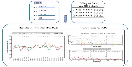
  • Four sets of constructed closure errors are within 0.30 ns, and their mean values are less than 0.15 ns, indicating that our estimated satellite DCBs of BDS-3 have high precision.
  • The RMS of receiver DCBs is mostly less than 1.50 ns with respect to CAS products. An obvious relationship is found between RMS values and the geographic latitude, e.g., the RMS of C1P-C5P DCB with more than 1.00 ns for stations in low latitude areas. Almost all the receivers of C1X/C5X/C7Z/C8X channels are located at middle and high latitudes, so the receiver DCBs are better consistent with CAS products.
  • The STDs of BDS-3 receiver DCBs are within 1.00 ns, which are not as stable as satellite DCBs. The STDs of different receiver types show no significant differences. However, the coefficients of ionospheric correction obtained by different frequencies differ significantly.
Although the BDS-2/3 system has been fully built, the number of stations with tracking new BDS-3 signals is far less than GPS. To promote precise applications of multi-frequency BDS-3, more stations with tracking full frequencies of BDS-3 signals need to be established, which will contribute to ionospheric modeling and DCBs estimation.

Author Contributions

Conceptualization of the Manuscript Idea: S.J. and Q.S. Methodology and Software: Q.S.; Supervision and Funding Acquisition: S.J.; Q.S. wrote the original draft preparation; S.J. reviewed and edited this paper. All authors have read and agreed to the published version of the manuscript.

Funding

This research was funded by National Natural Science Foundation of China (NSFC) Project, grant number 12073012.

Data Availability Statement

The BDS observation data from IGS MGEX networks can be obtained https://cddis.nasa.gov/archive/gps/data/daily/. The precise orbit products from GFZ are available at https://www.gfzpotsdam.de/GNSS/products/mgex/. The GIM products from CODE are available at https://cddis.nasa.gov/archive/gnss/products/ionex/. The DCB products provided by CAS and DLR can be obtained at https://cddis.nasa.gov/archive/gnss/products/bias/.

Acknowledgments

The authors thank IGS for providing the BDS observation data of MGEX networks, DLR/CAS for providing the DCB products, CODE for providing the GIM products, and GFZ for providing precise orbit products, as well as Ke Su and Zhenchuan Huang for their help with the English-language aspects of writing this paper.

Conflicts of Interest

The authors declare no conflict of interest.

References

  1. Wu, X.; Jin, S. GNSS-Reflectometry: Forest canopies polarization scattering properties and modeling. Adv. Space Res. 2014, 54, 863–870. [Google Scholar] [CrossRef]
  2. Jin, S.; Zhang, T. Terrestrial Water Storage Anomalies Associated with Drought in Southwestern USA from GPS Observations. Surv. Geophys. 2016, 37, 1139–1156. [Google Scholar] [CrossRef]
  3. Li, G.; Guo, S.; Lv, J.; Zhao, K.; He, Z. Introduction to global short message communication service of BeiDou-3 navigation satellite system. Adv. Space Res. 2021, 67, 1701–1708. [Google Scholar] [CrossRef]
  4. Yang, Y.; Mao, Y.; Sun, B. Basic performance and future developments of BeiDou global navigation satellite system. Satell. Navig. 2020, 1, 1. [Google Scholar] [CrossRef] [Green Version]
  5. Jin, S.; Su, K. PPP models and performances from single- to quad-frequency BDS observations. Satell. Navig. 2020, 1, 16. [Google Scholar] [CrossRef]
  6. Okoh, D.; Onwuneme, S.; Seemala, G.; Jin, S.; Rabiu, B.; Nava, B.; Uwamahoro, J. Assessment of the NeQuick-2 and IRI-Plas 2017 models using global and long-term GNSS measurements. J. Atmos. Sol.-Terr. Phys. 2018, 170, 1–10. [Google Scholar] [CrossRef]
  7. Li, M.; Yuan, Y.; Zhang, X.; Zha, J. A multi-frequency and multi-GNSS method for the retrieval of the ionospheric TEC and intraday variability of receiver DCBs. J. Geod. 2020, 94, 102. [Google Scholar] [CrossRef]
  8. Montenbruck, O.; Hauschild, A.; Steigenberger, P. Differential code bias estimation using multi-GNSS observations and global ionosphere maps. In Proceedings of the 2014 International Technical Meeting of the Institute of Navigation, San Diego, CA, USA, 27–29 January 2014; pp. 802–812. [Google Scholar]
  9. Chen, L.; Yi, W.; Song, W.; Shi, C.; Lou, Y.; Cao, C. Evaluation of three ionospheric delay computation methods for ground-based GNSS receivers. GPS Solut. 2018, 22, 125. [Google Scholar] [CrossRef]
  10. Li, W.; Wang, G.; Mi, J.; Zhang, S. Calibration errors in determining slant Total Electron Content (TEC) from multi-GNSS data. Adv. Space Res. 2019, 63, 1670–1680. [Google Scholar] [CrossRef]
  11. Zhang, B.; Ou, J.; Yuan, Y.; Li, Z. Extraction of line-of-sight ionospheric observables from GPS data using precise point positioning. Sci. China Earth Sci. 2012, 55, 1919–1928. [Google Scholar] [CrossRef]
  12. Liu, T.; Zhang, B.; Yuan, Y.; Zhang, X. On the application of the raw-observation-based PPP to global ionosphere VTEC modeling: An advantage demonstration in the multi-frequency and multi-GNSS context. J. Geod. 2019, 94, 1. [Google Scholar] [CrossRef]
  13. Zhang, B.; Teunissen, P.J.; Yuan, Y.; Zhang, X.; Li, M. A modified carrier-to-code leveling method for retrieving ionospheric observables and detecting short-term temporal variability of receiver differential code biases. J. Geod. 2019, 93, 19–28. [Google Scholar] [CrossRef] [Green Version]
  14. Su, K.; Jin, S.; Jiang, J.; Hoque, M.; Yuan, L. Ionospheric VTEC and satellite DCB estimated from single-frequency BDS observations with multi-layer mapping function. GPS Solut. 2021, 25, 68. [Google Scholar] [CrossRef]
  15. Klobuchar, J.A. Ionospheric Time-Delay Algorithm for Single-Frequency GPS Users. IEEE Trans. Aerosp. Electron. Syst. 1987, AES-23, 325–331. [Google Scholar] [CrossRef]
  16. Nava, B.; Coïsson, P.; Radicella, S.M. A new version of the NeQuick ionosphere electron density model. J. Atmos. Sol.-Terr. Phys. 2008, 70, 1856. [Google Scholar] [CrossRef]
  17. Yuan, Y.; Wang, N.; Li, Z.; Huo, X. The BeiDou global broadcast ionospheric delay correction model (BDGIM) and its preliminary performance evaluation results. NAVIGATION-J. Inst. Navig. 2019, 66, 55–69. [Google Scholar] [CrossRef] [Green Version]
  18. Li, Z.; Wang, N.; Liu, A.; Yuan, Y.; Wang, L.; Hernández-Pajares, M.; Krankowski, A.; Yuan, H. Status of CAS global ionospheric maps after the maximum of solar cycle 24. Satell. Navig. 2021, 2, 19. [Google Scholar] [CrossRef]
  19. Orus-Perez, R.; Nava, B.; Parro, J.; Kashcheyev, A. ESA UGI (Unified-GNSS-Ionosphere): An open-source software to compute precise ionosphere estimates. Adv. Space Res. 2021, 67, 56–65. [Google Scholar] [CrossRef]
  20. Yuan, Y.; Ou, J. A generalized trigonometric series function model for determining ionospheric delay. Prog. Nat. Sci. 2004, 14, 1010–1014. [Google Scholar] [CrossRef]
  21. Montenbruck, O.; Steigenberger, P.; Prange, L.; Deng, Z.; Zhao, Q.; Perosanz, F.; Romero, I.; Noll, C.; Stürze, A.; Weber, G.; et al. The Multi-GNSS Experiment (MGEX) of the International GNSS Service (IGS)—Achievements, prospects and challenges. Adv. Space Res. 2017, 59, 1671–1697. [Google Scholar] [CrossRef]
  22. Xue, J.; Song, S.; Zhu, W. Estimation of differential code biases for Beidou navigation system using multi-GNSS observations: How stable are the differential satellite and receiver code biases? J. Geod. 2016, 90, 309–321. [Google Scholar] [CrossRef]
  23. Zhu, Y.; Tan, S.; Feng, L.; Cui, X.; Zhang, Q.; Jia, X. Estimation of the DCB for the BDS-3 new signals based on BDGIM constraints. Adv. Space Res. 2020, 66, 1405–1414. [Google Scholar] [CrossRef]
  24. Li, M.; Yuan, Y. Estimation and Analysis of BDS2 and BDS3 Differential Code Biases and Global Ionospheric Maps Using BDS Observations. Remote Sens. 2021, 13, 370. [Google Scholar] [CrossRef]
  25. Wang, Q.; Jin, S.; Yuan, L.; Hu, Y.; Chen, J.; Guo, J. Estimation and Analysis of BDS-3 Differential Code Biases from MGEX Observations. Remote Sens. 2020, 12, 68. [Google Scholar] [CrossRef] [Green Version]
  26. Deng, Y.; Guo, F.; Zhang, X.; Liu, W. Estimation and analysis of the multi-frequency and multi-channel DCB for BDS-3. Acta Geod. Cartogr. Sin. 2021, 50, 448. [Google Scholar]
  27. Leick, A.; Rapoport, L.; Tatarnikov, D. GPS Satellite Surveying; John Wiley & Sons: Hoboken, NJ, USA, 2015. [Google Scholar]
  28. Jin, R.; Jin, S.; Feng, G. M_DCB: Matlab code for estimating GNSS satellite and receiver differential code biases. GPS Solut. 2012, 16, 541–548. [Google Scholar] [CrossRef]
  29. Ma, G.; Gao, W.; Li, J.; Chen, Y.; Shen, H. Estimation of GPS instrumental biases from small scale network. Adv. Space Res. 2014, 54, 871–882. [Google Scholar] [CrossRef]
  30. Schaer, S. Mapping and Predicting the Earth’s Ionosphere Using the Global Positioning System; Astronomical Institute, University of Berne: Bern, Switzerland, 1999. [Google Scholar]
  31. Schaer, S.; Gurtner, W.; Feltens, J. IONEX: The ionosphere map exchange format version 1. In Proceedings of the IGS AC workshop, Darmstadt, Germany, 9–11 February 1998. [Google Scholar]
  32. Wang, N.; Yuan, Y.; Li, Z.; Montenbruck, O.; Tan, B. Determination of differential code biases with multi-GNSS observations. J. Geod. 2016, 90, 209–228. [Google Scholar] [CrossRef]
  33. Jin, S.G.; Jin, R.; Li, D. Assessment of BeiDou differential code bias variations from multi-GNSS network observations. Ann. Geophys. 2016, 34, 259–269. [Google Scholar] [CrossRef] [Green Version]
  34. Ren, X.; Zhang, X.; Xie, W.; Zhang, K.; Yuan, Y.; Li, X. Global Ionospheric Modelling using Multi-GNSS: BeiDou, Galileo, GLONASS and GPS. Sci. Rep. 2016, 6, 33499. [Google Scholar] [CrossRef] [Green Version]
  35. Zhang, B.; Teunissen, P.J.G. Characterization of multi-GNSS between-receiver differential code biases using zero and short baselines. Sci. Bull. 2015, 60, 1840–1849. [Google Scholar] [CrossRef] [Green Version]
Figure 1. Distribution of MGEX stations with tracking the new BDS-3 signals.
Remotesensing 14 00594 g001
Figure 2. MP of the BDS-3 C19, C37, C38, and C45 satellites at stations PTGG (a) and FFMJ (b) during a period of 30 days.
Remotesensing 14 00594 g002
Figure 3. The mean bias and RMS of our estimated C1P-C5P, C1X-C5X, C1X-C7Z, and C1X-C8X, of BDS-3 satellite DCBs, with respect to the direct values provided by CAS products.
Remotesensing 14 00594 g003
Figure 4. The mean bias and RMS of our estimated C1X-C5X, C1X-C7Z, C1X-C8X, C5X-C7Z, C5X-C8X, and C7Z-C8X, of BDS-3 satellite DCBs, with respect to the conversion values provided by DLR products.
Remotesensing 14 00594 g004
Figure 5. DCB time series of BDS-3 C1P-C5P during a period of 30 days, and the differences time series with respect to CAS products.
Remotesensing 14 00594 g005
Figure 6. Distribution of deviations between nine DCB types of BDS-3 satellites and the corresponding mean values.
Remotesensing 14 00594 g006
Figure 7. Distribution of BDS-3 satellites C1P-C5P-C7D (a), C1X-C5X-C7Z (b), C1X-C5X-C8X (c), and C1X-C7Z-C8X (d) closure errors. The red line denotes the fitted normal distribution curve.
Remotesensing 14 00594 g007
Figure 8. Mean closure error of BDS-3 satellites C1P-C5P-C7D, C1X-C5X-C7Z, C1X-C5X-C8X, and C1X-C7Z-C8X.
Remotesensing 14 00594 g008
Figure 9. RMS error of the estimated BDS-3 receiver DCBs with respect to the products provided by CAS during the period of DOY 60–89 in 2021.
Remotesensing 14 00594 g009
Figure 10. Statistics for RMS error of the estimated BDS-3 receiver DCBs with respect to the products provided by CAS during the period of DOY 60–89 in 2021.
Remotesensing 14 00594 g010
Figure 11. Distribution of STDs for all BDS-3 receiver DCB types of C1P/C5P/C7D channels (a) and C1X/C5X/C7Z/C8X channels (b) during the period of DOY 60–89 in 2021. Receiver index is arranged according to the classification and order in Table 4. The digitals represent coefficients of the ionospheric correction with corresponding DCB types.
Remotesensing 14 00594 g011
Table 1. The pseudorange channels of BDS multi-frequency signals.
SystemFreq. BandFrequency/MHzChannel Codes
of Pseudorange
BDS-2B21207.140C7I C7Q C7X
BDS-2/3B11561.098C2I C2Q C2X
B31268.52C6I C6Q C6X
BDS-3B1C1575.42C1D C1P C1X
B2a1176.45C5D C5P C5X
B2b1207.140C7D C7P C7Z
B2(a+b)1191.795C8D C8P C8X
Table 2. Nine types in the DCB estimation of BDS-3.
Freq. BandPseudorange Observation Channels
Combination 1Stations NumberCombination 2Stations Number
B1C-B2aC1P-C5P60C1X-C5X28
B1C-B2bC1P-C7D43C1X-C7Z23
B2a-B2bC5P-C7D42C5X-C7Z23
B1C-B2(a + b) C1X-C8X21
B2a-B2(a + b) C5X-C8X23
B2b-B2(a + b) C7Z-C8X19
Table 3. Mean STD of BDS-3 DCBs of DLR, CAS, and our results, showing the corresponding satellite psuedo random noise (PRN); the bold types are the direct values provided by CAS products.
TypeCASDLROur Results
MaxMinMeanMaxMinMeanMaxMinMean
C1P-C5P0.115
(C42)
0.040
(C39)
0.076 0.100
(C42)
0.049
(C39)
0.072
C1P-C7D 0.087
(C34)
0.045
(C38)
0.066
C5P-C7D 0.036
(C43)
0.013
(C26)
0.025
C1X-C5X0.128
(C30)
0.050
(C40)
0.0870.470
(C45)
0.065
(C40)
0.1250.195
(C37)
0.050
(C27)
0.092
C1X-C7Z0.118
(C36)
0.056
(C40)
0.0920.465
(C45)
0.079
(C44)
0.1300.168
(C37)
0.049
(C30)
0.091
C5X-C7Z0.120
(C36)
0.035
(C40)
0.0750.215
(C39)
0.073
(C36)
0.1110.075
(C37)
0.023
(C27)
0.042
C1X-C8X0.131
(C46)
0.066
(C40)
0.0970.490
(C45)
0.080
(C35)
0.1290.191
(C37)
0.043
(C27)
0.095
C5X-C8X0.117
(C44)
0.039
(C40)
0.0710.213
(C39)
0.065
(C36)
0.1040.052
(C22)
0.016
(C23)
0.029
C7Z-C8X0.085
(C22)
0.021
(C40)
0.0550.093
(C43)
0.040
(C24)
0.0600.051
(C29)
0.011
(C40)
0.022
Table 4. Station and receiver information for BDS-3 DCB estimation.
Observation ChannelsReceiver TypeStation
C1P/C5P/C7DSEPT POLARX5TRAMC4BREWBRUXCEBRGAMGGODE
HARBKOUGMGUENLIBNNORONSA
PARKSPT0STJ3THTGUSN7YEL2
SEPT POLARX5ABPOALICAREGARUCCHPIDGAR
FAA1FALKGOP6HAL1IISCJPLM
KIR0KIRUKITGKOURMAL2MAO0
MAR6MDO1METGMIZUMKEANKLG
NYA2OUS2PTGGQAQ1REDUSANT
SCORSEYGSUTHTHU2USUDVACS
VILLVIS0
SEPT POLARX5EKOS1
SEPT ASTERX4KIT3RIO2TASH
C1X/C5X/C7Z/C8XTRIMBLE ALLOYBRSTCHPGLMMFOWMGUNB3
JAVAD TRE_3 DELTAARHTBRMGFFMJGCGOGODNGODS
HUEGLEIJMET3PIE1SOD3TIT2
WARNWTZZ
JAVAD TRE_3ENAOLPGSPOTSSGOCSUTMULAB
URUMWINDWUH2
Publisher’s Note: MDPI stays neutral with regard to jurisdictional claims in published maps and institutional affiliations.

