High-Resolution Seamless Daily Sea Surface Temperature Based on Satellite Data Fusion and Machine Learning over Kuroshio Extension

Abstract

Sea SurfaceTemperature (SST) is a critical parameter for monitoring the marine environment and understanding various ocean phenomena. While SST can be regularly retrieved from satellite data, it often suffers from missing data due to various reasons including cloud contamination. In this study, we proposed a novel two-step data fusion framework for generating high-resolution seamless daily SST from multi-satellite data sources. The proposed approach consists of (1) SST reconstruction based on Data Interpolate Convolutional AutoEncoder (DINCAE) using the SSTs derived from two satellite sensors (i.e., Moderate Resolution Imaging Spectroradiometer (MODIS) and Advanced Microwave Scanning Radiometer 2(AMSR2)), and (2) SST improvement through data fusion using random forest for consistency with in situ measurements with two schemes (i.e., scheme 1 using the reconstructed MODIS SST variables and scheme 2 using both MODIS and AMSR2 SST variables). The proposed approach was evaluated over the Kuroshio Extension in the Northwest Pacific, where a highly dynamic SST pattern can be found, from 2015 to 2019. The results showed that the reconstructed MODIS and AMSR2 SSTs through DINCAE yielded very good performance with Root Mean Square Errors (RMSEs) of 0.85 and 0.60 °C and Mean Absolute Errors (MAEs) of 0.59 and 0.45 °C, respectively. The results from the second step showed that scheme 2 and scheme 1 produced RMSEs of 0.75 and 0.98 °C and MAEs of 0.53 and 0.68 °C, respectively, compared to the in situ measurements, which proved the superiority of scheme 2 using multi-satellite data sources. Scheme 2 also showed comparable or even better performance than two operational SST products with similar spatial resolution. In particular, scheme 2 was good at simulating features with fine resolution (~50 km). The proposed approach yielded promising results over the study area, producing seamless daily SST products with high quality and high feature resolution.

1. Introduction

Sea Surface Temperature (SST) is an important driver and tracer of the global atmosphere and ocean circulations in terms of air–sea interaction [1,2,3,4]. Satellite-derived SST has been widely used in ocean studies due to its extensive spatiotemporal coverage, such as the monitoring of oceanfront, eddy, and turbulence [5,6,7,8,9]. Two types of satellite sensors have been used to retrieve SST: thermal infrared and passive microwave sensors. Thermal infrared sensors (e.g., Advanced Very High-Resolution Radiometer (AVHRR) and Moderate Resolution Imaging Spectroradiometer (MODIS)) provide relatively high spatial (i.e., 1 km) and temporal (i.e., subdaily) resolution SST data. However, they often suffer from cloud contamination, sun glint effect, and aerosols, resulting in missing data especially in the Western Pacific Ocean. While passive microwave sensors (e.g., Advanced Microwave Scanning Radiometer 2 (AMSR2)) are much less influenced by atmospheric conditions to estimate SST, they provide relatively low spatial (i.e., 25 km) resolution data [10].

Satellite-based SST often loses a large amount of data for various reasons mentioned above, limiting the production of seamless daily SST from single satellite data sources. Therefore, studies to reconstruct missing SST data have been actively conducted [11,12,13,14,15,16,17,18]. Several widely used seamless daily SST products are based on Optimal Interpolation (OI) with data assimilation of multiple infrared and passive microwave satellite observations and in situ measurements, which include global products from Danish Meteorological Institute (DMI) on a grid scale of 0.05° and Operational Sea Surface Temperature and Sea Ice Analysis (OSTIA) on a grid scale of 0.054° [16,17,18,19]. However, since such operational products are based on the OI approach resulting in smoothed surface, they have a relatively limited feature resolution [17]. Several processes such as outlier removals and smoothing are conducted to improve the accuracy of the operational SST products, which often degrade the spatial pattern of the products, even though 1 km SST data are assimilated in the products [18]. The feature resolution of OI-based SST products is often greater than 100 km in horizontal resolution in the Power Spectral Density (PSD) analysis [15]. The Multiscale Ultra-high-Resolution Sea Surface Temperature (MUR SST) provides the global SST data on a 0.01° grid resolution and proves a relatively higher feature resolution than other OI-based operational SST products [15]. While seamless daily SST products generate high-quality SST fields for operational purposes, several error corrections for improving the consistency with in situ measurements (e.g., buoys and ship measurements) have been conducted [20].

In addition to OI, the Empirical Orthogonal Function (EOF) has been used to interpolate satellite SST time series, demonstrating an acceptable performance (root mean square error (RMSE) ~ 1.07 °C) [13,14]. Data Interpolate Empirical Orthogonal Function (DINEOF) is one of the most cutting-edge reconstruction methods of geophysical ocean parameters [21,22,23,24]. However, DINEOF has suffered from the smoothing of mesoscale features due to the high missing rate of satellite data and the truncation of EOF [17,25]. Furthermore, conventional OI and EOF approaches have numerous assumptions on linearity in handling sparsely distributed data, which makes it hard to reflect complicated nonlinear ocean dynamics during the interpolation process.

Recently, machine learning has emerged as a cutting-edge technology for the reconstruction and estimation of ocean data, which can resolve the nonlinear relationship among high-dimensional and heterogeneous data [26,27,28,29,30,31,32,33]. A variety of machine learning techniques for reconstructing SST have been evaluated, including Artificial Neural Network (ANN), the patch-based NN with Kalman filter, and Random Forest (RF) [18,32,34]. More recently, deep learning has been used to reconstruct satellite-derived SST. Barth et al., (2020) proposed Data Interpolate Convolutional AutoEncoder (DINCAE), which uses a convolutional AutoEncoder (AE) structure based on OI [25]. While conventional OI is based on a linear assumption (e.g., the best linear unbiased estimator), DINCAE applies nonlinear interpretation of OI through a series of convolutional operations. AE in the DINCAE algorithm can effectively extract meaningful features from irregular and sparsely distributed data through dimension reduction, similar to EOF. Therefore, DINCAE showed relatively higher restoration accuracy than DINEOF in Provençal Sea (4.56–9.5° E and 39.5–44.43° N) in the Mediterranean [25]. In addition, DINCAE simulates higher spatiotemporal variability of SST than DINEOF. Han et al., (2020) adopted DINCAE for the first time to reconstruct satellite-derived chlorophyll-a concentrations and examined the use of multiple satellite data as input variables to DINCAE [35]. Since DINCAE has not been used to reconstruct SST based on multiple input data, there is a chance to further improve the reconstruction accuracy of SST. In addition, multiple satellite sensors can be synergistically used to generate high-resolution seamless daily SST.

This research aims to produce spatially seamless daily SST with high spatial and feature resolution and consistency with in situ SST measurements through the synergistic use of two satellite sensor data based on machine learning. The proposed approach consists of two parts: (1) the reconstruction (i.e., gap filling) of two SST products (i.e., one from a thermal infrared sensor and the other from a passive microwave sensor) using DINCAE, and (2) the improvement of the reconstructed SSTs using in situ measurements and RF machine learning. The specific objectives of this study were to (1) design a framework to produce high-resolution satellite-based seamless daily SST based on DINCAE and random forest machine learning using two satellite data and in situ measurements, (2) evaluate the proposed models from both quantitative and qualitative aspects including their generalization over the Kuroshio Extension in the Northwest Pacific, where a highly dynamic SST pattern can be found, from 2015 to 2019, and (3) analyze the feature resolution of SST generated using the proposed approach.

2. Study Area and Data

2.1. Study Area

The study area is the Kuroshio Extension (KE) region of the Northwest Pacific (latitude 25–45° N and longitude 120–170° E; Figure 1a). The KE region has gained a high attention as the physical characteristics (i.e., heat flux and eddy variability) of the region are closely related to the climate of the Northwest Pacific [36,37,38]. The northward flowing warm Kuroshio current encounters the southward cold subpolar Oyashio current, generating vigorous meanders flowing eastward in the Northwest Pacific region [39,40]. The high eddy kinetic energy induced by recirculation results in the intensified spatiotemporal variability of turbulent flows (i.e., eddy, front) in the KE system. The spatial variability of SST in the region has strong seasonal and interannual characteristics [41]. Therefore, KE was selected to evaluate the proposed framework to produce high-resolution seamless daily SST in a highly dynamic region. The study area was divided into six equal zones (hereafter, tiles; Figure 1b) to reduce the computational demand of the proposed approach. A buffer of 20 pixels was applied to each tile to effectively combine the tiles after reconstruction. The study period is five years from 2015 to 2019.

2.2. Satellite and In Situ Data

In this study, we used daily data from MODIS onboard the AQUA satellite and AMSR2 onboard the Global Change Observation Mission 1st–Water (GCOM–W1) satellite at the same equatorial crossing local time (i.e., 1:30 p.m. for the ascending pass and 1:30 a.m. for the descending pass). The vertical variability of SST (i.e., from skin to foundation SST) is high during the daytime due to the varied levels of insolation. However, the vertical structure of temperature is relatively stable at night [42,43]. Thus, we focused on night-time SST (i.e., local time at 1:30 a.m.) to reduce the impact of diurnal heating on the ocean’s upper layer in the daytime when using in situ measurements as reference data.

We used the night-time MODIS Short-Wave Sea Surface Temperature (SST4) in this study. The night-time MODIS SST4 (hereafter, SST) is generated using shortwave infrared channels (i.e., 3.95 and 4.05 μm) based on the split window Nonlinear SST (NLSST) algorithm [44]. Since the shortwave infrared channels are less affected from atmospheric absorption and have higher spectral sensitivity than long-wave infrared channels (i.e., 11.03 and 12.02 μm) at night [45]. The night-time SST4 data were binned and mapped into an equidistant cylindrical projection on a 4 km resolution grid for 5 years from 2015 to 2019 and were downloaded from NASA Physical Oceanography Distributed Active Archive Center (PODAAC) (https://podaac.jpl.nasa.gov/dataset/) (accessed on 24 June 2021).

AMSR2 provides global passive microwave-based (PMW) sub-skin (i.e., 1 mm) SST data. AMSR2 SST is retrieved using the brightness temperature (BT) measured at 6.9 and 10.7 GHz with vertical polarization. The vertical polarization is less affected by wind than the horizontal polarization [46]. This study used SST retrieved using BT at 6.9 GHz with vertical polarization because the 10.7 GHz data have larger radiometric noise and geophysical errors at high latitudes and cold water than 6.9 GHz [47,48]. The AMSR2 SST data on a 10 km resolution grid for 5 years from 2015 to 2019 were downloaded from the Japan Aerospace Exploration Agency (https://gcom-w1.jaxa.jp) (accessed on 26 June 2021).

Figure 2 shows the spatial and temporal missing percentages of AMSR2 and MODIS SSTs. Since AMSR2 (i.e., passive microwave) is relatively less affected by clouds, the overall missing rate per day (i.e., the temporal missing rate of 42.96% for AMSR2) is lower than that of MODIS (i.e., 71.84%). The spatial missing rate of MODIS dramatically increased above 30° N, resulting in less than 20% of data available for the study period from 2015 to 2019.

Among various in situ SST data sources, drifting buoys have been widely used to validate numerous satellite-derived SSTs due to the measurement depth close to the surface that satellite sensors observe [7]. Drifting buoys measure sea water temperature at around 20 cm below the sea surface, while satellite-based SSTs are retrieved from 1μm (i.e., thermal infrared) to 1 mm (i.e., passive microwave) below the surface. Although the measurement depth is slightly different between drifting buoy- and satellite-based SST, there is a strong correlation between drifting buoy measurements and satellite-based SSTs [49]. In this study, the hourly buoy observations were obtained by National Oceanic and Atmospheric Administration Observing System Monitoring Center (NOAA OSMC) via Global Telecommunication System (GTS) (https://www.aoml.noaa.gov/phod/gdp/real-time_data.php) (accessed on 10 September 2021). A total of 265,926 in situ SSTs were collected from 390 drifters from 1 January 2015, to 31 December 2019. The spatial distribution of the number of in situ SST observations (i.e., drifting buoys) within the study boundary is depicted in Figure 1c. It is necessary to minimize the bias caused by the different measurement depths between satellite-based and in situ SSTs. Thus, we added 0.17 °C to the MODIS SST to reduce the cool skin effect and subtracted 0.03 °C from the AMSR2 SST to mitigate warm bias at night [28,50,51,52]. Finally, the proposed approach was applied to the bias-corrected satellite SSTs at a depth of 20 cm.

3. Methods

Figure 3 shows a framework of the proposed approach to generate high-quality, high-resolution seamless daily SST from two satellite sensor data. The proposed approach consists of two parts: (1) reconstruction of MODIS and AMSR2 SSTs based on DINCAE and (2) improvement of the reconstructed SST through data fusion based on RF machine learning using in situ measurements. Two parts were described in the following sections in details.

3.1. Reconstruction of SST

The AMSR2 SST data with 10 km resolution were resampled to the 4 km grid of MODIS SST using the nearest neighbor method to ensure the same grid unit. We extracted 50 occlusion masks (i.e., missing data areas of the original AMSR2 SSTs) for the first 50 days of the study period to evaluate both the reconstructed MODIS and AMSR2 SSTs [25,35]. The 50 occlusion masks were applied to both MODIS and AMSR2 SSTs on randomly selected 50 days (i.e., same days on both MODIS and AMSR2 but excluding the first 50 days) during the study period. After occlusion, the MODIS and AMSR2 SSTs (i.e., every tile) were fed into DINCAE (see Section 3.1.1), the reconstruction model adopted in this study. More details about DINCAE were described in Section 3.1.1.

After the SST reconstruction, we mosaicked the six tiles to produce a spatially continuous SST field. A postprocessing was conducted to minimize the SST discrepancy in the tile boundaries. The discrepancy typically occurs due to the zero-padding of the convolution layers in DINCAE [25]. Among the overlapped 20 pixels by tile, the outer 5 pixels were removed because they contained the artifacts due to zero-padding. Then, the remaining 15 pixels were used to minimize the SST discrepancy in the tile boundaries based on distance-based weights using an exponential function (Equation (1)).

$$DW=\frac{1}{1+exp\left[ D\times \pm W\right]}$$

(1)

where DW is the distance-based weight; D represents the number of the overlapped horizontal pixels (i.e., 30 pixels); and W represents the empirical weight to organize the inclination of the exponential function. Through multiple tests, the optimal weight was determined as 0.3. This postprocessing was applied in all directions of the adjacent tiles (i.e., up, down, left, and right).

3.1.1. Data INterpolate Convolutional AutoEncoder (DINCAE)

The DINCAE algorithm developed by Barth et al., (2020) was applied to reconstruct daily MODIS and AMSR2 SSTs [25]. The basic model architecture of DINCAE is a stacked AE, which stacks multiple convolutional layers on the encoder and decoder layers in a self-supervised way. In addition, DINCAE adopts the denoising AE concept that contributes to the robustness of AE as a generative model [53]. DINCAE corrupts input data with noise and learns a feature representation (i.e., information of SST) to minimize the difference between the corrupted data and input data. DINCAE divides random subsets (i.e., for optimization) from minibatches, which are used as independent validation data for every epoch. This is a different learning strategy compared to the conventional AE.

A total of 10 input variables were used in DINCAE, including SST anomalies and the inverse of error variance as key input data, which are the same as the previous research [25,35] (

Table 1. Summary of input variables used in DINCAE to reconstruct MODIS and AMSR2 SSTs in this study.

Variable Type	Variable
Satellite data derived (MODIS/AMSR2)	- SST anomalies scaled by the inverse of the error variance (the scaled anomaly is zero when data are in an absence)
	- Inverse of the error variance (zero when data are in an absence)
	- Scaled SST anomalies of the previous day
	- Inverse of error variance of the previous day
	- Scaled SST anomalies of the next day
	Inverse of error variance of the next day
Auxiliary variables	- Longitude (scaled linearly between −1 and 1)
	- Latitude (scaled linearly between −1 and 1)
	- Cosine of the day of the year divided by 365.25
	- Sine of the day of the year divided by 365.25

).

The training process of DINCAE is based on OI, which aims to minimize the analysis error (i.e., between the estimated and observed values). The basic OI approach can be found in the previous studies [25,54,55]. DINCAE estimates the anomaly of SST (${\widehat{y}}_{ij}$) from the inverse of the error variance and provides the error standard deviation (${\widehat{\sigma }}_{ij}$) of the reconstructed SST field. This estimated error standard deviation (${\widehat{\sigma }}_{ij}$) represents a relatively quantified error of the reconstructed SST. The anomaly of SST and the error standard deviation are the outputs from DINCAE as two layers. The first layer $T_{ij1}$ is the logarithm of the inverse of the expected error variance; the second layer $T_{ij2}$ is the temperature anomaly divided by the error variance. The corresponding error variance (${\widehat{\sigma }}_{ij}^2$) is calculated from the logarithmic function of the inverse of the expected error variance ($T_{ij1}$). The reconstructed SST ($R_{ij}$) is the sum of the reconstructed anomaly (${\widehat{y}}_{ij}$) and mean of the time-series SST ($m$). All parameters are computed as:

$${\widehat{\sigma }}_{ij}^2=\frac{1}{max\left(exp\left(min\left(T_{ij1}, \gamma \right)\right),\delta \right)}$$

(2)

$${\widehat{y}}_{ij}=T_{ij2}\ast {\widehat{\sigma }}_{ij}^2$$

(3)

$$R_{ij}={\widehat{y}}_{ij}+m$$

(4)

where $\gamma =10$ and $\delta ={10}^{-3} °{\mathrm{C}}^{-2}$. The subscripts $i$ and $j$ indicate every grid location (i.e., $T_{ij1}$ and $T_{ij2}$ are produced for every grid). The $max$ and $min$ in Equation (2) indicate maximum and minimum functions. The effective range of the error standard deviation is expected from 0 to 1 °C because the expected error standard deviation is scaled by error variance [25].

During optimization, DINCAE occluded the input data using randomly chosen masks (i.e., randomly select SSTs from minibatch) of missing data areas at every minibatch. The occluded data from chosen masks were used for calculating loss to optimize the model. The loss function ($J({\widehat{y}}_{ij},{\widehat{\sigma }}_{ij}^2)$) of DINCAE assumes two outputs (i.e., $T_{ij1}$, $T_{ij2}$) to be the parameters (i.e., estimated mean, estimated standard deviation) with Gaussian probability distribution. The anomaly of SST (${\widehat{y}}_{ij}$) and the error standard deviation (${\widehat{\sigma }}_{ij}$) are the mean of the estimation and standard deviation with Gaussian probability distribution, respectively. The loss function ($J({\widehat{y}}_{ij},{\widehat{\sigma }}_{ij}^2)$) is calculated as Equation (5):

$$J\left({\widehat{y}}_{ij},{\widehat{\sigma }}_{ij}^2\right)=\frac{1}{2N}{\displaystyle \sum }_{ij}\left[{\left(\frac{y_{ij}-{\widehat{y}}_{ij}}{{\widehat{\sigma }}_{ij}}\right)}^2+\mathit{log}\left({\widehat{\sigma }}_{ij}^2\right)+2\mathit{log}\left(\sqrt{2\pi }\right)\right]$$

(5)

where $y_{ij}$ and $N$ are the occluded data of each grid and the number of occluded data during optimization, respectively. The first term is the mean square error, which is scaled by the error standard deviation. The second term reduces the variance of error standard deviation to penalize overestimation. The third term is a constant for normalization (i.e., Neglect term). Therefore, parameters (i.e., weight and bias) are determined to maximize the likelihood (i.e., in the form of Gaussian probability distribution) between estimations and observations. Since the loss function is related to both anomaly estimation (i.e., expected error variance) and expected error estimation, DINCAE has the advantage of providing reliable performance in terms of reconstruction and error estimation.

DINCAE is independent of an inherent error of SST data (i.e., sensor malfunctioning and synoptic error at satellite overpass time), background error (i.e., first guess), and the error between the observation and first guess (i.e., unbiased, averaged error is zero). It is only affected by analysis error from the model [13,25]. More details about DINCAE are found in Barth et al., (2020) [25]. The dimension of the input dataset to DINCAE is 1826 ∗ 480 ∗ 720 ∗ 10 before dividing the study area into the six tiles (i.e., length of the study period, latitude, longitude, and input variables, respectively). The DINCAE package was provided by Geohydrodynamics and environment research Github (https://github.com/gher-ulg/DINCAE) (accessed on 10 October 2021). All experiments were run on a computer with Intel(R) Xeon(R) Silver 4215R CPU @ 3.20GHz and NVidia Quadro RTX 8000 GPU (48 GB of memory). The hyperparameter settings of DINCAE determined based on the empirical testing of various combinations are summarized in

Table 2. The hyperparameters used to train DINCAE in this study. The values in bold indicate the optimized (selected) hyperparameter values. The range of numerical values in the parentheses was empirically tested for parameter optimization.

Hyper-Parameters	Options
Window of timeseries SST	3 days (±3–7 days)
Epoch	800–1000 (Stop with the lowest error)
Standard deviation of the noise	1 (0.9–1.1)
Error standard deviation of the observations	0.05
Image (transposed convolutional layer) resize method in the decoder layers	Nearest neighbor
Pooling method in the decoder layers	Average
Number of convolution layers of the encoder and decoder	4/4 (1–4)
Batch size	64 (50–128)
Skip-connection between the encoder and decoder	4
Dropout rate during optimization	0.3
Number of filters for the encoder and decoder layers (from left to right for the encoder layers, and the opposite for the decoder layers)	16/24/36/54 (16–128)
Dropout rate in the latent space	0.2 (0.1–0.3)
Activation function for convolutional layers	Leaky ReLu
L2 regularization weight	0.001
Optimizer	Adam
Learning rate of step size in the optimizer	1 × 10−3
The exponential decay rate for the first moment (i.e., beta 1) in the optimizer	0.9

.

3.2. Data Fusion for Improving Reconstructed SST

The second part of the proposed approach is to generate a high-quality (i.e., strong consistency with in situ measurements), high-resolution seamless daily SST based on the bias and variance correction through the data fusion of the reconstructed SSTs targeting in situ measurements using RF. The primary assumption of this part is that in situ measurements are regarded as the reference data of the reconstructed SSTs (see Section 2.2).

The input variables of RF are described in

Table 3. Summary of the input variables used in the random forest model to further improve the reconstructed SSTs through data fusion.

Variable Type	Variable
In situ data (Target variable)	- GTS drifting buoys
DINCAE outputs (MODIS/AMSR2, input variables)	- Estimated SST (Mean SST add with anomaly SST calculate from SST scaled by the inverse of the expected error variance and logarithm of the inverse of the expected error variance)
	- Expected error standard deviation from the logarithm of the inverse of the expected error variance
Auxiliary variables (Input variables)	- Latitude (Scaled linearly between −1 and 1)
	- Sine of the day of the year divided by 365.25
	- Presence of data (If value = 1, data are missing; otherwise, data are valid)

. The outputs (reconstructed SST and error standard deviation) of DINCAE (see Section 3.1.1), presence of original data, latitude, and scaled Day Of Year (DOY) as input variables in the RF model (Table 3). The presence of data (i.e., binary) was selected to distinguish the reconstructed and original SST pixels in RF [30]. Latitude affects the retrieval of satellite-based SST, temporal variability of SST, and the number of in situ matchup data [28,30,32]. Scaled DOY was used to document the seasonality of SST [25,28]. In this data fusion process, two schemes (S1 and S2) were evaluated: S1 uses the MODIS-based reconstructed SST and its error standard deviation, and three auxiliary variables. S2 uses the reconstructed SST and error terms from both MODIS and AMSR2, and three auxiliary variables. Learning the relationship between the estimated SST (i.e., reconstructed SST) and the error standard deviation of the estimated SST might expect to further improve the accuracy of the reconstructed SST because the literature [25] shows a high correlation between the estimated SST and the error standard deviation.

Random Forest (RF)

In this study, RF was used to correct the bias and variance between the reconstructed SST and in situ drifting buoy data. Note that the bias caused by the different measurement depth was corrected for the satellite-derived SSTs (refer to 2.2). RF has been widely used to examine the regression problems of ocean parameters in recent years [26,27,28,30,31,32,56]. RF is a nonparametric ensemble approach that composes a multitude of bootstrapped regression trees [57,58,59,60,61]. Ensemble regression trees have different bootstrap data (bagging), and each tree’s nodes are expended toward the least error of constructing the tree. RF calculates a mean of squared residuals (i.e., mean of square error) from aggregated trees using simple averaging for internal validation of the RF model. RF was implemented using Python through the scikit statistical analysis package (https://scikit-learn.org) (accessed on 10 October 2021). In this study, the optimal number of trees was determined as 500, and the depth of tree was set as 50 through a multitude of empirical testing.

3.3. Performance Evaluation of the Proposed Approach

We conducted an accuracy assessment for each part: using occlusion masks as validation data for the SST reconstruction part and using Leave-One-Year-Out-Cross-Validation (LOYOCV) for the improvement of the reconstructed SST through data fusion. For LOYOCV, one year of in situ data were held out from the training, and the remaining data were used to develop a model. Then, the held-out data were used to evaluate the model. This process was repeated for the five years. LOYOCV was conducted to assess the two schemes (S1 and S2) for the second part.

For accuracy assessments, the coefficient of determination (R²; Equation (6)), bias (Equation (7)), Root Mean Square Error (RMSE) (Equation (8)), relative RMSE (rRMSE; Equation (9)), and Mean Absolute Error (MAE) (Equation (10)) were used to evaluate the performance of the models for both parts of the proposed approach. For further quantitative assessment using in situ measurements, an adjusted relative mean absolute error (ARMAE) (Equation (11)) was calculated based on LOYOCV results [62,63,64,65].

$$R^2=1-\frac{{\sum }_{i=1}^n{\left( y_i-\widehat{y_i}\right)}^2}{{\sum }_{i=1}^n{\left( y_i-\overline{y_i}\right)}^2}, \overline{y_i}=\frac{{\sum }_{i=1}^n{y}_i}{n}$$

(6)

$$Bias \left(°\mathrm{C}\right)= {\displaystyle \sum }_{i=1}^n\frac{\left(\widehat{y_i}-y_i\right)}{n}$$

(7)

$$RMSE \left(°\mathrm{C}\right)=\sqrt{\frac{{\sum }_{i=1}^n{\left(\widehat{y_i}-y_i\right)}^2}{n}}$$

(8)

$$rRMSE \left(\%\right)=\frac{100 \ast RMSE}{\overline{y_i}}$$

(9)

$$MAE \left(°\mathrm{C}\right)=\frac{1}{n}{{\displaystyle \sum }}_{i=1}^n\left|\widehat{y_i}-y_i\right|$$

(10)

$$ARMAE=\frac{1}{n}{{\displaystyle \sum }}_{i=1}^n\frac{\left(\left|\widehat{y_i}-y_i\right|-OE\right)}{\left|y_i\right|}$$

(11)

where $y_i$ is the observed value,$\widehat{y_i}$ is the predicted value, $y_{max}$ and $y_{min}$ represent the maximum and minimum values of reference SST data, and n is the number of samples. The expression $\left(\left|\widehat{y_i}-y_i\right|-OE\right)$ of $ARMAE$ is set zero for negative values. $OE$ is an estimated average value of the systematic error of in situ measurements. In this study, $OE$ was identified as 0.015 °C using the collected drifting buoy data (i.e., GTS) [66,67,68,69].

For further qualitative and quantitative assessment of the high-resolution SST field generated from the proposed approach focusing on various ocean features, we used a gradient field and PSD. The gradient of the SST field is often used to describe ocean phenomena such as ocean fronts and currents [41]. PSD has been widely used to define the eddy kinetic energy of mesoscale ocean turbulence [17,41]. First, the magnitude of gradient field ($G$) is given as follows (Equation (12)):

$$G=\sqrt{{\left[\left[\begin{array}{ccc}-1& 0& +1\\ -2& 0& +2\\ -1& 0& +1\end{array}\right]\ast S÷\left(2\times d_x\right)\right]}^2+{\left[\left[\begin{array}{ccc}-1& -2& -1\\ 0& 0& 0\\ 1& 2& 1\end{array}\right]\ast S÷\left(2\times d_y\right)\right]}^2}$$

(12)

where the first and second terms are a zonal (Horizontal) and meridional (Vertical) gradients, respectively. The square matrix of each term are the 3 × 3 convolutional operator of zonal and meridional Sobel filters, respectively. $S$ is the SST field. The $d_x$ and $d_y$ are a longitudinal and latitudinal distances (i.e., pixel size) of each SST, respectively, which are 4 (i.e., equidistant). Second, PSD is based on Fast Fourier Transform (FFT). FFT converts a turbulence-domain (i.e., spatial) representation of a function into frequency domain. In this study, we calculated the wavenumber of the SST field and set the output resolution to 4 km × 4 km.

4. Results and Discussion

4.1. Performance of SST Reconstruction

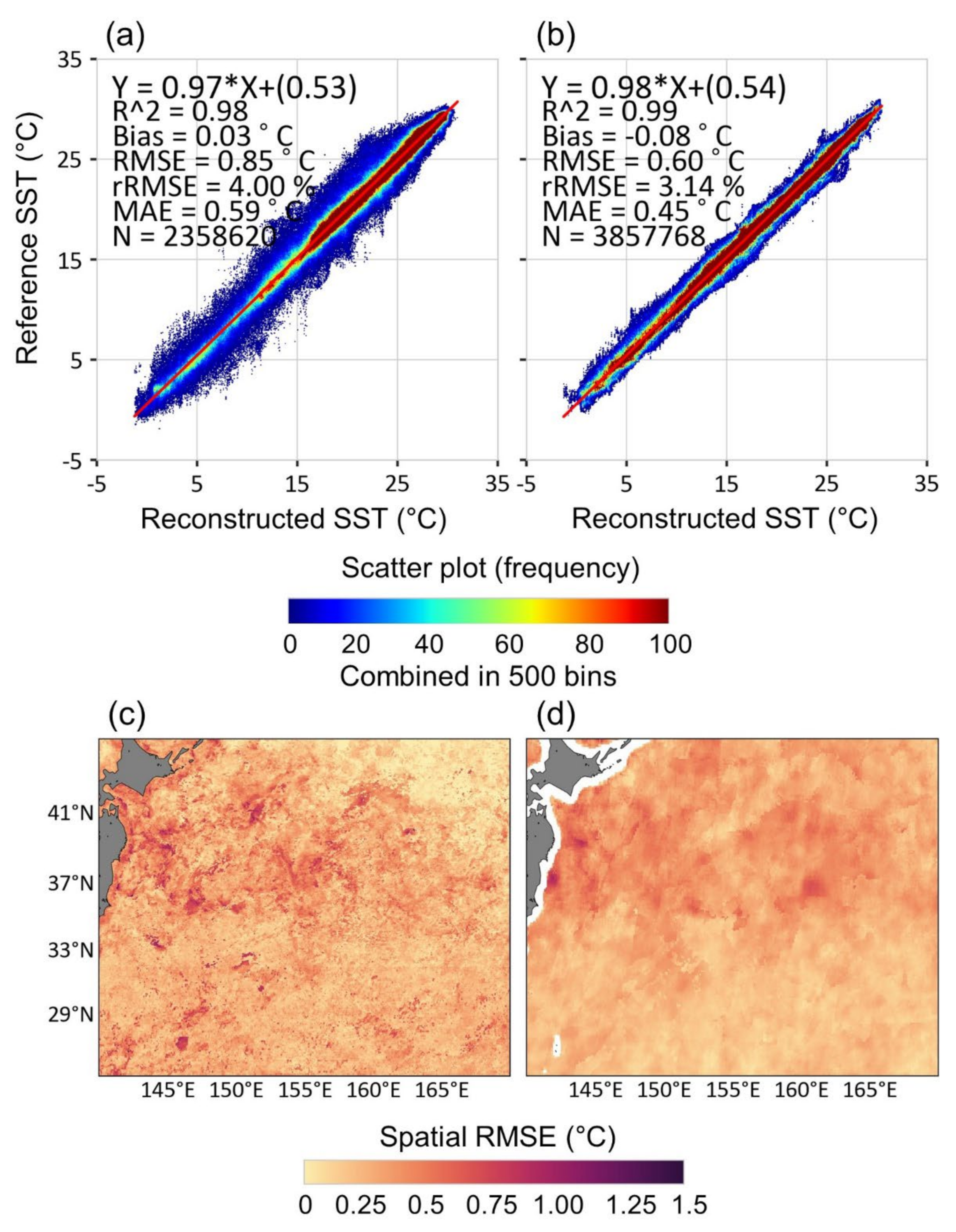
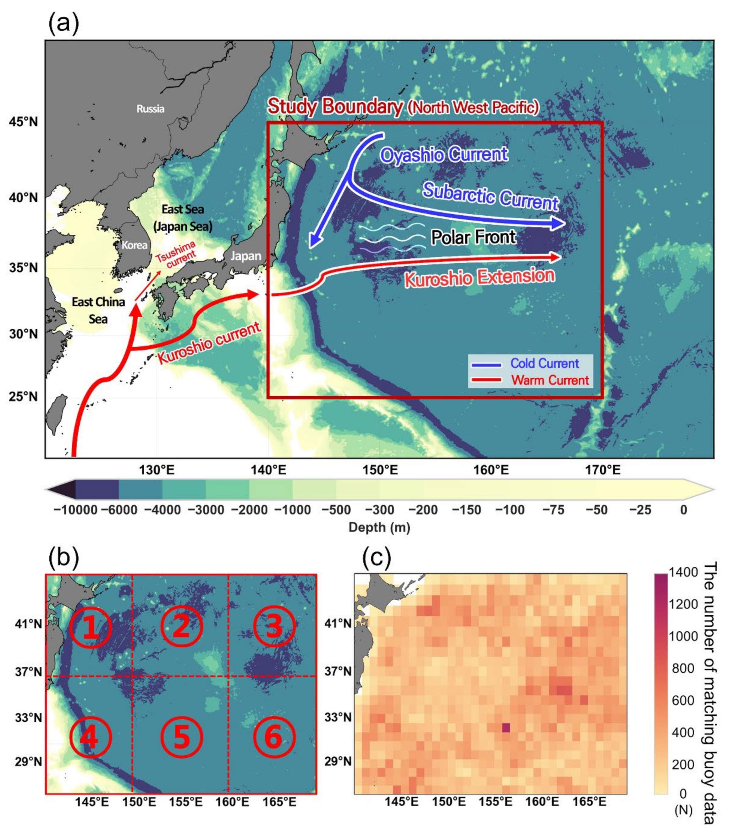
Figure 4 shows the validation results of the MODIS and AMSR2 SSTs reconstructed through DINCAE. While both resulted in similar R² (0.98 for MODIS and 0.99 for AMSR2) and bias (0.03 °C for MODIS and –0.09 °C for AMSR2), the reconstructed AMSR2 SST produced slightly better performance metrics than the MODIS one in terms of RMSE, rRMSE, and MAE by 0.25 °C, 0.86%, and 0.14 °C, respectively (Figure 4a,b). The reconstructed MODIS SST was relatively underestimated and had a slightly higher variance when compared to the reconstructed AMSR2 SST. The different performances between the two reconstructed SSTs were possibly due to differences in missing data rates, spatial resolution, and the number of SST training samples [7,70].

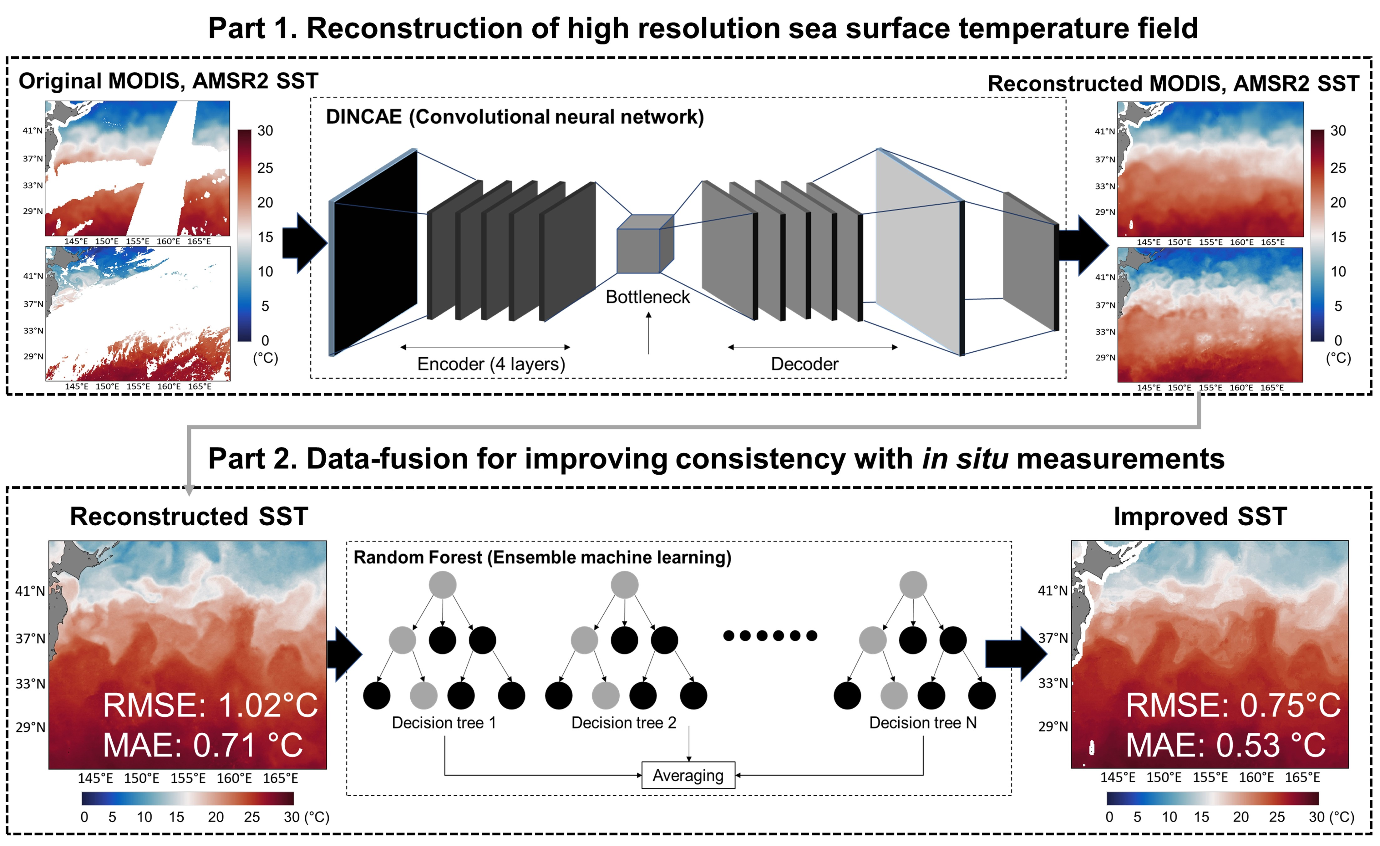
The reconstructed MODIS and AMSR2 SSTs showed the RMSE distribution between 0.1 and 0.7 °C across the study area. Both results have higher RMSE distribution (~0.7 °C) in tiles 1–3 (i.e., high latitudes; refer to Figure 2b) than tiles 4–6 (Figure 4c,d). This corresponds to the results by tile using the optimized parameters (Table S2). In addition, high RMSE (>1.0 °C) was found near the land (e.g., tile 1; Figure 4c,d). This high error near the shelf region corresponds to the results of Han et al., (2020), where DINCAE was applied to reconstruct chlorophyll concentrations in coastal areas. The study pointed out that river discharge and external factors such as marine activities affected the distribution of chlorophyll-a and SST, increasing the reconstruction error [35]. Therefore, one possible reason of high error near the land in the present study is high spatiotemporal variability of SST due to the west boundary current (i.e., Kuroshio current), which limited the anomaly estimation of DINCAE in the coastal areas [35]. In addition, the swath characteristic of AMSR2 affected the spatial distribution of RMSE along with missing data regions (145–150° E in Figure 4d).

Table 4. Validation accuracy of the MODIS and AMSR2 SST reconstructions for each tile.

Satellite	The Number of Tiles	Coefficient of Determination (R2)	Bias (°C)	RMSE (°C)	rRMSE (%)	MAE (°C)	The Number of Data
MODIS	1	0.98	0.01	1.12	7.72	0.79	321,128
	2	0.98	0.08	1.10	6.57	0.81	298,132
	3	0.98	−0.31	0.98	5.94	0.73	186,952
	4	0.98	0.04	0.76	3.17	0.53	526,838
	5	0.98	0.07	0.65	2.67	0.44	545,800
	6	0.98	−0.18	0.69	2.85	0.50	479,770
AMSR2	1	0.99	0.43	0.85	5.83	0.66	471,262
	2	0.99	−0.24	0.78	5.42	0.61	566,431
	3	0.99	0.20	0.67	4.79	0.51	713,314
	4	0.99	0.11	0.50	2.17	0.38	664,447
	5	0.99	0.01	0.45	1.92	0.33	660,315
	6	0.99	−0.00	0.38	1.63	0.30	781,999

presents the accuracy assessment results of the reconstruction models by tile. Interestingly, tiles 1–3 at high latitudes performed less than tiles 4–6 at low latitudes (Δ0.3 °C in RMSE, Δ1% in rRMSE, and Δ0.15 °C in MAE for MODIS; and Δ0.3 °C in RMSE, Δ1% in rRMSE, and Δ0.15 °C in MAE for AMSR2). Accuracy difference by latitude possibly resulted from the difference in the range of SST during the study period. The SST range that DINCAE estimated was 35 °C (from –4 to 31 °C) for tiles 1–3, while 21 °C (from 11 to 32 °C) for tiles 4–6, which affected the model performance (Figure S1).

Table 5. Accuracy of the original and reconstructed SST pixels for MODIS and AMSR2 when compared to the in situ measurements.

Satellite	Pixels	Coefficient of Determination (R2)	Bias (°C)	RMSE (°C)	rRMSE (%)	MAE (°C)	ARMAE	The Number of Data (N)
MODIS	Original SST pixels	0.99	−0.31	0.76	3.42	0.53	0.023	73,023
	Reconstructed SST pixels	0.98	−0.35	1.10	5.96	0.78	0.041	189,398
	Total (i.e., original + reconstructed SST pixels)	0.98	−0.34	1.02	5.21	0.71	0.036	262,421
AMSR2	Original SST pixels	0.99	−0.12	0.83	4.36	0.60	0.031	142,557
	Reconstructed SST pixels	0.98	−0.20	0.85	4.22	0.62	0.030	119,864
	Total (i.e., original + reconstructed SST pixels)	0.99	−0.15	0.84	4.30	0.61	0.031	262,421

summarizes the accuracy of the original SST and reconstructed SST pixels (i.e., estimated SST from DINCAE), when compared to the in situ measurements. Both MODIS and AMSR2 SSTs showed high correlation ($R^2$ = 0.98–0.99) with in situ measurements. The original MODIS SST pixels showed higher accuracy than the original AMSR2 SST when compared to in situ measurements by RMSE of 0.07 °C, rRMSE of 0.94%, MAE of 0.07 °C, and ARME of 0.008. The reconstructed MODIS SST pixels resulted in less accuracy (RMSE = 1.1 °C, rRMSE = 5.96%, MAE = 0.78 °C, and ARMAE = 0.041) against in situ data than the original MODIS one (RMSE = 0.76 °C, rRMSE = 3.42%, MAE = 0.53 °C, and ARMAE = 0.023). On the other hand, the reconstructed AMSR2 SST pixels yielded accuracy similar to the original AMSR2 one.

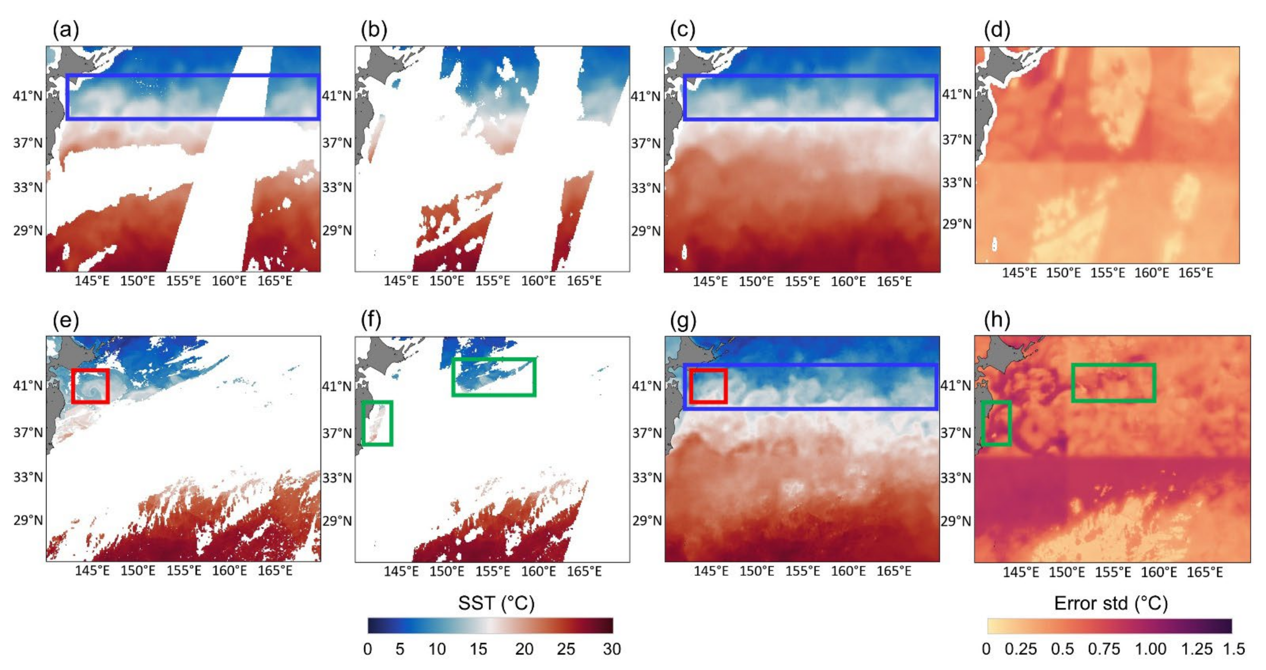
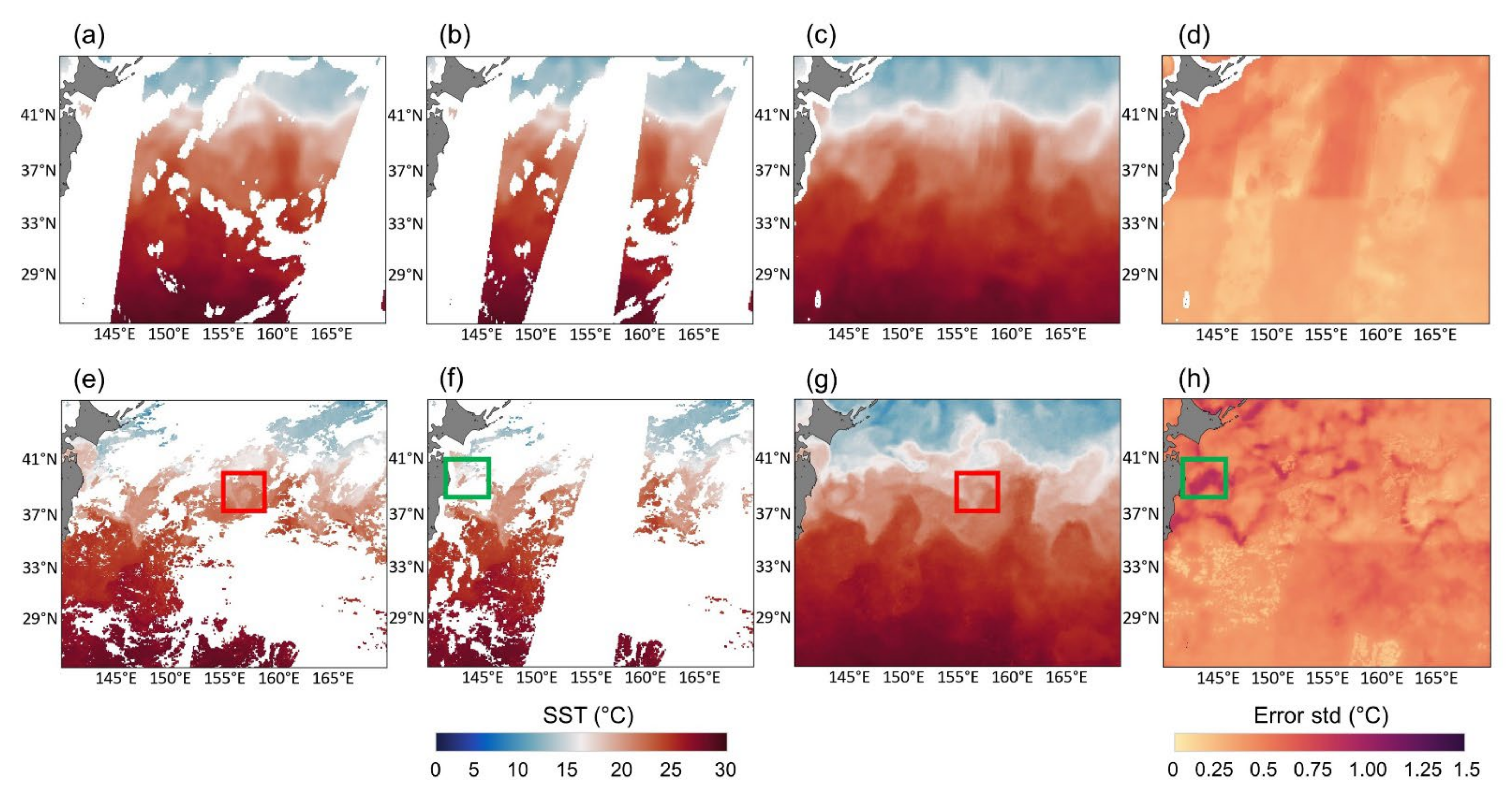
Figure 5 and Figure 6 show the examples of the original SST, the original SST with the occlusion mask for validation, the reconstructed SST, and its error standard deviation for both MODIS and AMSR2 on 25 May 2015, and 6 November 2018, respectively. Overall, DINCAE well simulated the spatial distribution of SST for both MODIS and AMSR2. Due to the coarse resolution of AMSR2, the result did not show the detailed SST patterns but produced relatively good reconstruction in the occluded areas (Figure 5a–c; Figure 6a–c; Figure S2). In particular, the MODIS SST after reconstruction clearly showed ocean features such as eddies (i.e., mesoscale features < 100 km) and a polar front (blue boxes in Figure 5a,c,g). However, smoothing occurred for fine-scale features (i.e., sub-mesoscale features < 50 km) such as a warm core ring edge of an eddy (red box in Figure 5e,g). DINCAE results in dimension reduction while extracting features from SST data through the pooling convolutional layers. When DINCAE reconstructs the reduced data to the original dimension using the nearest resampling, smoothing often occurs, and some fine feature information disappears [25]. While skip connection to keep the characteristics of the original data was applied to mitigate the smoothing problem, smoothing still remained, affecting the performance of reconstruction at the fine feature scale (i.e., submesoscale).

As shown in Figure 5 and Figure 6, the error standard deviation of AMSR2 SST was low (<1 °C) over the study area including the areas with missing data. Similar to other accuracy metrics, the difference in the error standard deviation by latitude was also dominant in the reconstructed AMSR2 SST (Figure 5f and Figure 6f). OI-based DINCAE generally yielded relatively low errors for areas where data exist similar to the results of AMSR2 (Figure 5f and Figure 6f). On the other hand, the error standard deviation of the reconstructed MODIS SST varied by tile and the difference by latitude was not great. Some areas at high latitude (tiles 1–3) where original SST data exist yielded the high error standard deviation for the reconstructed MODIS SST (green boxes in Figure 5f,h; Figure 6f,h). The scaled error probability density function of MODIS was positively skewed, while that of AMSR2 followed the normal distribution (Figure S3), which made the MODIS reconstruction slightly less performed than the AMSR2 one. In addition, both AMSR2 and MODIS results showed high error standard deviation in the coastal region of Japan regardless of the presence of data, which was similar to the spatial distribution of RMSE (Figure 4c,d). These results imply that areas with low reconstruction accuracy had large uncertainty in the estimation of reliable error standard deviation. Such an uncertainty has been reported in the previous studies that applied OI for EOF [13].

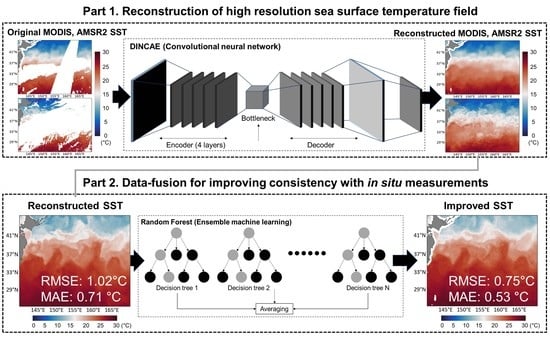
4.2. Improvement of the Reconstructed SST

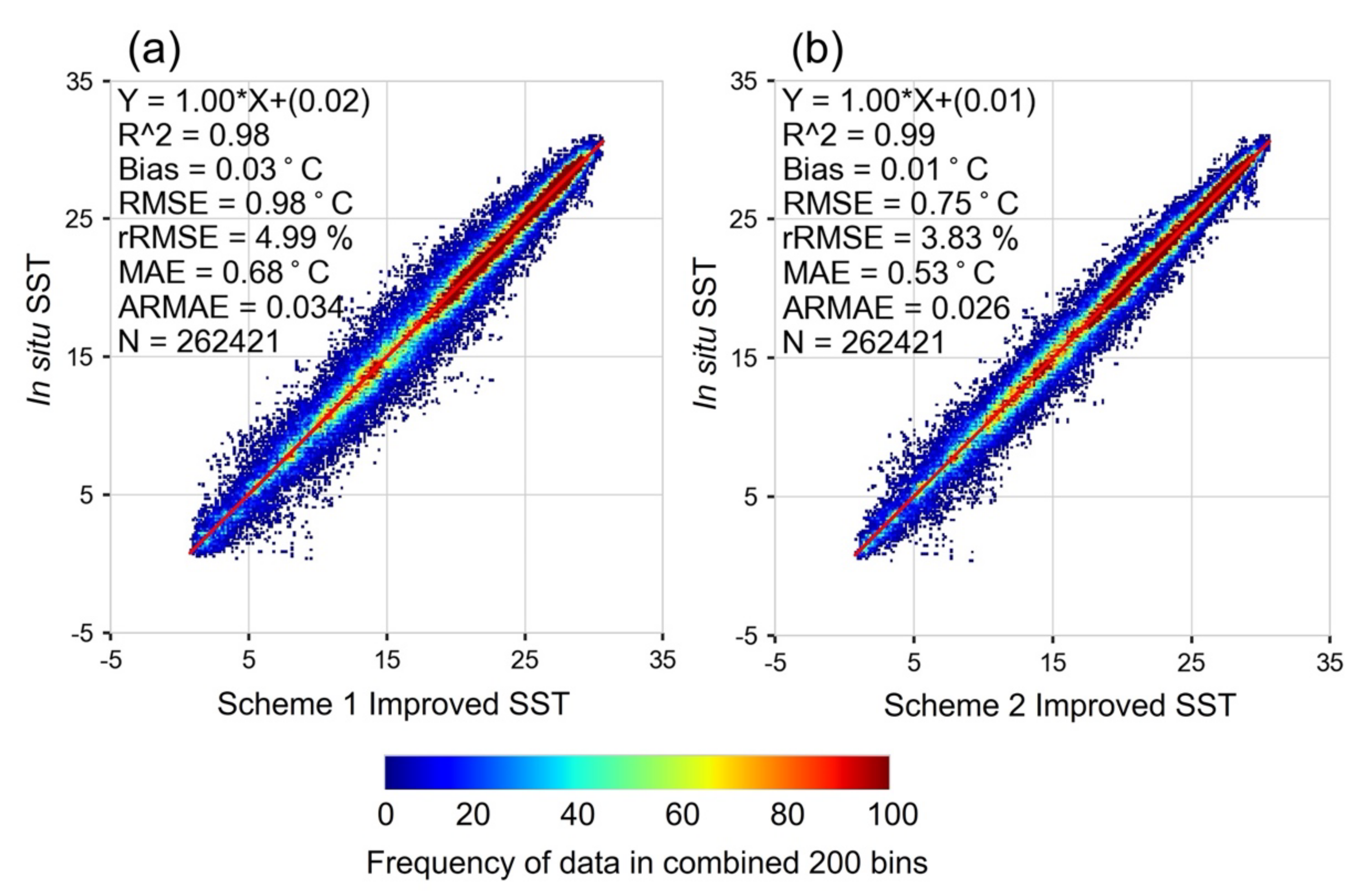
Figure 7 presents the accuracy assessment results of the data fusion model to improve SST using RF for schemes 1 and 2. It should be noted that both Scheme 1 and Scheme 2 showed better performance than the original and reconstructed MODIS SSTs (Figure 7; Table 5). Scheme 2 that used multi-satellite data outperformed scheme 1 based on a single satellite data source, yielding higher accuracy metrics (Scheme 2: $R^2$ = 0.99, Bias = 0.01 °C, RMSE = 0.75 °C, rRMSE = 3.83%, MAE = 0.53 °C and ARMAE = 0.026; Scheme 1: $R^2$ = 0.98, Bias = 0.02 °C, RMSE = 0.98 °C, rRMSE = 4.99%, MAE = 0.68 °C and ARMAE = 0.034). This implies that the synergistic use of both the reconstructed MODIS and AMSR2 SSTs improved the accuracy generating a more similar SST product to in situ data.

Table 6. Accuracy metrics of Leave-One-Year-Out-Cross-Validation (LOYOCV) results of schemes 1 and 2, scheme 2 calibration results, and OSTIA SST when compared to in situ data.

SST	Validation Area (i.e., Pixels)	Coefficient of Determination (R2)	Bias (°C)	RMSE (°C)	rRMSE (%)	MAE (°C)	ARMAE	The Number of Data (N)
Scheme 1	Original MODIS SST pixels	0.99	0.04	0.74	3.31	0.51	0.022	73,023
Scheme 1	Reconstructed MODIS SST pixels	0.98	0.02	1.05	5.70	0.74	0.039	189,398
Scheme 2	Original MODIS SST pixels	0.99	0.04	0.58	2.61	0.41	0.018	73,023
Scheme 2	Reconstructed MODIS SST pixels	0.99	0.00	0.80	4.35	0.57	0.030	189,398
Scheme 2 (Calibration)	The entire study area	1.00	0.00	0.09	0.46	0.04	0.002	262,421
OSTIA	The entire study area	0.99	0.05	0.52	2.65	0.32	0.016	262,421

compares scheme 1 LOYOCV results, scheme 2 LOYOCV results, and scheme 2 calibration results to the operational gap-free OSTIA SST product using in situ measurements. The accuracy of scheme 1 SST over both the original and reconstructed SST pixels produced a minor accuracy increment when compared to the MODIS SST (Table 6). Similarly, the proposed scheme 2 approach yielded a similar performance regardless of the presence of the original AMSR2 SST pixels (Figure S4). Interestingly, the accuracy of the scheme 2 approach over the reconstructed pixels of MODIS SST was similar to that of the original MODIS SST (Table 5 and Table 6), which implies that the data fusion approach successfully increased the accuracy of SST for data missing areas. According to ARMAE [63] (Table S1), scheme 2 showed excellent performance for both the original and reconstructed SST when compared to the MODIS SST and scheme 1 (Table 5 and Table 6).

Notably, the LOYOCV accuracy of scheme 2 over the original MODIS SST pixels is comparable to the accuracy of OSTIA SST (Table 6). Since the OSTIA model corrected the error of SST using GFS drifting buoy data, which are the same in situ measurements used in this study. While the accuracy of OSTIA over the study area was very similar (RMSE of 0.59 °C) to those reported in the literature [16], scheme 2 calibration outperformed the OSTIA SST (Δ0.43 °C in RMSE, Δ2.19% in Rrmse, Δ0.28 °C in MAE, and Δ0.014 in ARMAE). Consequently, the proposed scheme 2 approach integrating two satellite data sources can produce the high-quality SST product comparable (or even better) to the operational SST product that incorporates multiple satellite and in situ data.

4.3. Feature Resolution Analysis

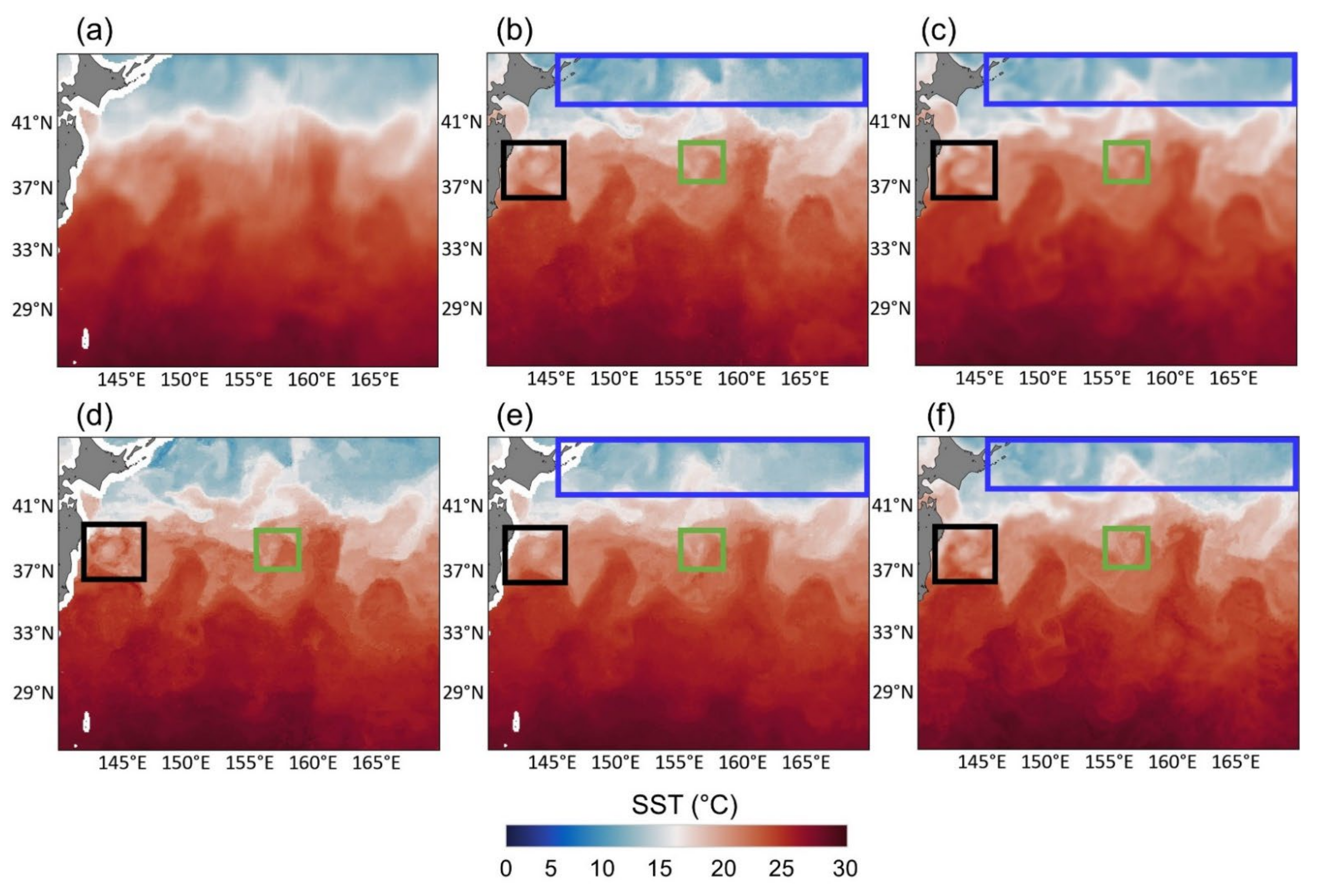
Figure 8 depicts the spatial distribution of the reconstructed SSTs, SSTs improved through data fusion by scheme using bias-corrected satellite-SSTs (i.e., MODIS and AMSR2 SSTs, see Section 2.2), and high-resolution operational SST products. As shown in Figure 4a and Figure S3a, the reconstructed MODIS SST (Figure 8b) tends to be underestimated at high latitude (i.e., blue boxes in Figure 8b,c,e,f) when compared to other products. One possible reason is that the image resizing method (i.e., nearest neighbor) in the decoder layer for dimension restoration induces smoothness during the reconstruction [35]. Surprisingly, scheme 1 (Figure 8d) and scheme 2 (Figure 8e) effectively mitigated such underestimation in the reconstructed MODIS SST (Figure 8b). In particular, scheme 1 (Figure 8d) seemed to focus on a specific range of temperature when compared to the reconstructed MODIS SST (Figure 8b). For example, the scheme 1 result (Figure 8d) clearly showed the core ring of a warm eddy (i.e., black boxes on Figure 8), similar to the operational products (OSTIA in Figure 8c and MUR SST in Figure 8f). However, based on visual interpretation, the overall spatial distribution of scheme 2 SST was in better agreement with the operational products than that of scheme 1 SST, which corresponded to the accuracy assessment results in Table S3.

However, the comma-shaped rotational features at the end of warm cores (i.e., green boxes in Figure 8) in the operational products were not clearly shown in the reconstructed and scheme 1-/scheme 2-improved SST results. As mentioned in Figure 5 and Figure 6, it is challenging to effectively reconstruct SST through DINCAE at the submesoscale [35]. Scheme 1 and 2 models were also affected by the reconstructed SSTs, which were used as input variables in the models.

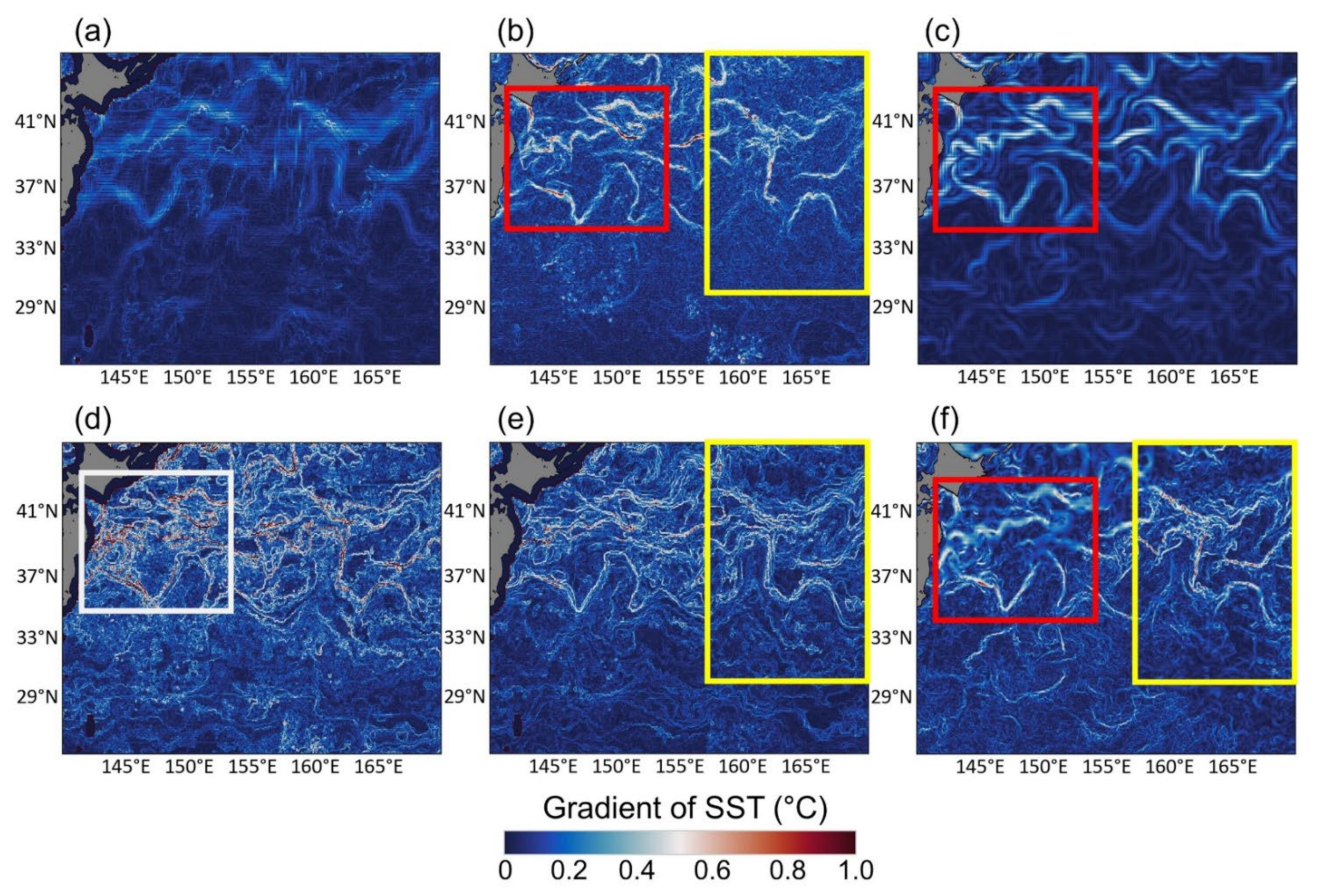
Figure 9 depicts the gradient fields of the reconstructed SSTs, the scheme-improved SSTs, and operational SST products. It is not possible to quantitatively compare the gradient fields as they are different by interpolation approach. Thus, a comparison was conducted using the super resolution (i.e., 1 km) MUR SST product as reference data. The reconstructed MODIS SST (Figure 9b) showed overall similar gradients to MUR SST (Figure 9f). In particular, scheme 2-improved SST (Figure 10e) showed much more similar gradients to the MUR SST in the open sea (i.e., yellow box in Figure 9) than the reconstructed MODIS SST (Figure 9b). Scheme 2-improved SST resulted in more detailed gradients than OSTIA (Figure 9c), comparable to MUR SST.

However, the gradient fields of both scheme-improved SSTs (Figure 9d,e) had more diverged patterns compared to that of the reconstructed MODIS SST (Figure 9b). In particular, the scheme 1 result (Figure 9d) had more excessively diverged gradients (i.e., noise in the white box in Figure 9d) than the scheme 2 result (Figure 9e). One possible reason is that since RF works pixel-by-pixel, the relationships among the neighboring SST pixels might not be well trained. The incorporation of textual information might be able to mitigate the problem [71].

Interestingly, the high error standard deviation in the reconstructed MODIS SST in the east coast of Japan (i.e., tile 1 in Figure 5h and 6h) had a similar distribution with the gradient fields of the reconstructed MODIS SST (i.e., red boxes in Figure 9b). This implies that DINCAE, the reconstruction model adopted in this study, might have high uncertainty in the areas where there is high spatiotemporal variability of SST (i.e., rapid change due to west-boundary current).

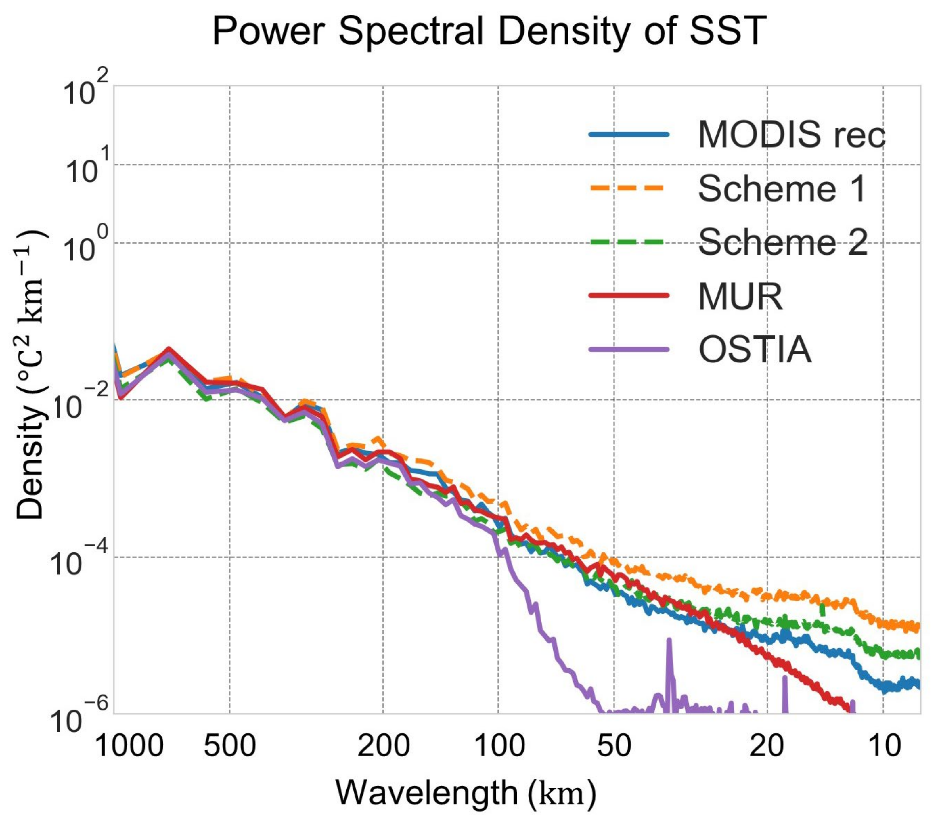
Figure 10 compares the PSDs of the reconstructed MODIS SST, the scheme-improved SSTs, and two operational SST products. All SSTs, except for OSTIA, resulted in a similar turbulence significant energy especially for fine-scale (<50 km) ocean surface phenomena [15]. OI-based OSTIA was able to simulate SST at the scale of 100 km [15,17,18]. The density of scheme 1-improved SST was higher than those of other high-resolution SSTs including the density of the reference MUR SST. This is possibly due to the excessive diverged gradients generated in the scheme 1 model, increasing false turbulence, which degraded feature resolution (Figure 9d). The scheme 2-improved SST generated very similar density with the MUR SST, especially at scales between 20 and 100 km, which implies that the proposed approach can successfully simulate the seamless SST at high resolution (~4 km).

4.4. Novelty and Limitations

Many previous SST reconstruction studies have focused on the restoration of missing data, which did not fully consider the consistency with in situ measurements [17,18,25,34,35]. To our knowledge, only Sunder et al., 2020, has used in situ data as a target to generate the high-resolution cloud-free daily SST, but it lacks discussion of restoring the ocean phenomena such as fronts and eddies [32]. This study proposed a novel method that improves consistency with in situ SST measurements and generates the fine resolution seamless daily SST field through the synergistic use of two satellite sensor data based on machine learning. In particular, the proposed method shows a very promising result when compared to the high-resolution operational SST products using various assessment methods from both quantitative and qualitative aspects.

There are, however, several limitations of the proposed method. First, the proposed approach tends to rely on the performance of DINCAE. Although DINCAE applied skip connection to keep the fine feature scale of ocean phenomena of the original data, it was not able to fully mitigate the smoothing problem. DINCAE also has uncertainty in estimating a reliable error standard deviation over areas with a low reconstruction accuracy. Another limitation is that the pixel-wise learning adopted in the second part of the proposed approach may cause diverged gradients without consideration of textual information.

5. Conclusions

In this study, we proposed a data fusion approach for generating high-resolution seamless daily SST based on machine learning (i.e., DINCAE and RF) over the Kuroshio Extension in the Northwest Pacific from 2015 to 2019. MODIS and AMSR2 SSTs were reconstructed through DINCAE. Then, the reconstructed SSTs were fused with ancillary data through RF targeting in situ measurements with two schemes (scheme 1 using the reconstructed MODIS SST variables and scheme 2 using both MODIS and AMSR2 SST variables). The results showed that the reconstructed MODIS and AMSR2 SSTs through DINCAE yielded very good performance with the RMSEs of 0.85 and 0.60 °C and MAE of 0.59 and 0.45 °C, respectively. In the second step, scheme 2 clearly outperformed scheme 1 by Bias of 0.01 °C, RMSE of 0.23 °C, rRMSE of 1.16%, and MAE of 0.15 °C based on LOYOCV. Scheme 2 also showed comparable or even better performance than operational SST products with similar spatial resolution. In particular, scheme 2 was good at simulating features with fine resolution (~50 km) such as MUR SST. The proposed approach yielded promising results over KE, producing seamless daily SST products with high quality and high feature resolution (i.e., low-power spectral density at low wavelengths). This study deserves further investigation, including the use of an attention mechanism in the deep learning model and the evaluation of the model transferability.

References

1. Dunstan, P.K.; Foster, S.D.; King, E.; Risbey, J.; O’Kane, T.J.; Monselesan, D.; Hobday, A.J.; Hartog, J.R.; Thompson, P.A. Global patterns of change and variation in sea surface temperature and chlorophyll a. Sci. Rep. 2018, 8, 14624. [Google Scholar] [CrossRef] [PubMed] [Green Version]
2. Park, S.; Deser, C.; Alexander, M.A. Estimation of the surface heat flux response to sea surface temperature anomalies over the global oceans. J. Clim. 2005, 18, 4582–4599. [Google Scholar] [CrossRef] [Green Version]
3. Podestá, G.P.; Glynn, P.W. Sea surface temperature variability in Panamá and Galápagos: Extreme temperatures causing coral bleaching. J. Geophys. Res. Ocean. 1997, 102, 15749–15759. [Google Scholar]
4. Samelson, R.; Skyllingstad, E.; Chelton, D.; Esbensen, S.; O’Neill, L.; Thum, N. On the coupling of wind stress and sea surface temperature. J. Clim. 2006, 19, 1557–1566. [Google Scholar]
5. Brasnett, B.; Colan, D.S. Assimilating retrievals of sea surface temperature from VIIRS and AMSR2. J. Atmos. Ocean. Technol. 2016, 33, 361–375. [Google Scholar] [CrossRef]
6. Cummings, J.A. Operational multivariate ocean data assimilation. Q. J. R. Meteorol. Soc. 2005, 131, 3583–3604. [Google Scholar] [CrossRef] [Green Version]
7. O’Carroll, A.G.; Armstrong, E.M.; Beggs, H.M.; Bouali, M.; Casey, K.S.; Corlett, G.K.; Dash, P.; Donlon, C.J.; Gentemann, C.L.; Høyer, J.L. Observational needs of sea surface temperature. Front. Mar. Sci. 2019, 6, 420. [Google Scholar] [CrossRef]
8. Tory, K.J.; Dare, R.A. Sea surface temperature thresholds for tropical cyclone formation. J. Clim. 2015, 28, 8171–8183. [Google Scholar] [CrossRef]
9. Vazquez-Cuervo, J.; Torres, H.S.; Menemenlis, D.; Chin, T.; Armstrong, E.M. Relationship between SST gradients and upwelling off Peru and Chile: Model/satellite data analysis. Int. J. Remote Sens. 2017, 38, 6599–6622. [Google Scholar] [CrossRef]
10. Wentz, F.J.; Gentemann, C.; Smith, D.; Chelton, D. Satellite measurements of sea surface temperature through clouds. Science 2000, 288, 847–850. [Google Scholar] [CrossRef] [Green Version]
11. Barth, A.; Beckers, J.-M.; Troupin, C.; Alvera-Azcárate, A.; Vandenbulcke, L. divand-1.0: N-dimensional variational data analysis for ocean observations. Geosci. Model Dev. 2014, 7, 225–241. [Google Scholar] [CrossRef] [Green Version]
12. Barth, A.; Troupin, C.; Reyes, E.; Alvera-Azcárate, A.; Beckers, J.-M.; Tintore, J. Variational interpolation of high-frequency radar surface currents using DIVAnd. Ocean Dyn. 2021, 71, 293–308. [Google Scholar] [CrossRef]
13. Beckers, J.-M.; Barth, A.; Alvera-Azcárate, A. DINEOF reconstruction of clouded images including error maps–application to the Sea-Surface Temperature around Corsican Island. Ocean Sci. 2006, 2, 183–199. [Google Scholar]
14. Beckers, J.-M.; Rixen, M. EOF calculations and data filling from incomplete oceanographic datasets. J. Atmos. Ocean. Technol. 2003, 20, 1839–1856. [Google Scholar] [CrossRef]
15. Chin, T.M.; Vazquez-Cuervo, J.; Armstrong, E.M. A multi-scale high-resolution analysis of global sea surface temperature. Remote Sens. Environ. 2017, 200, 154–169. [Google Scholar] [CrossRef]
16. Donlon, C.J.; Martin, M.; Stark, J.; Roberts-Jones, J.; Fiedler, E.; Wimmer, W. The operational sea surface temperature and sea ice analysis (OSTIA) system. Remote Sens. Environ. 2012, 116, 140–158. [Google Scholar] [CrossRef]
17. Fablet, R.; Viet, P.H.; Lguensat, R. Data-driven Models for the Spatio-Temporal Interpolation of satellite-derived SST Fields. IEEE Trans. Comput. Imaging 2017, 3, 647–657. [Google Scholar]
18. Ouala, S.; Fablet, R.; Herzet, C.; Chapron, B.; Pascual, A.; Collard, F.; Gaultier, L. Neural network based Kalman filters for the Spatio-temporal interpolation of satellite-derived sea surface temperature. Remote Sens. 2018, 10, 1864. [Google Scholar] [CrossRef] [Green Version]
19. Høyer, J.L.; Le Borgne, P.; Eastwood, S. A bias correction method for Arctic satellite sea surface temperature observations. Remote Sens. Environ. 2014, 146, 201–213. [Google Scholar] [CrossRef]
20. Good, S.; Fiedler, E.; Mao, C.; Martin, M.J.; Maycock, A.; Reid, R.; Roberts-Jones, J.; Searle, T.; Waters, J.; While, J. The current configuration of the OSTIA system for operational production of foundation sea surface temperature and ice concentration analyses. Remote Sens. 2020, 12, 720. [Google Scholar] [CrossRef] [Green Version]
21. Alvera-Azcárate, A.; Barth, A.; Parard, G.; Beckers, J.-M. Analysis of SMOS sea surface salinity data using DINEOF. Remote Sens. Environ. 2016, 180, 137–145. [Google Scholar] [CrossRef] [Green Version]
22. Alvera-Azcárate, A.; Barth, A.; Beckers, J.M.; Weisberg, R.H. Multivariate reconstruction of missing data in sea surface temperature, chlorophyll, and wind satellite fields. J. Geophys. Res. Ocean. 2007, 112. [Google Scholar]
23. Hilborn, A.; Costa, M. Applications of DINEOF to satellite-derived chlorophyll-a from a productive coastal region. Remote Sens. 2018, 10, 1449. [Google Scholar] [CrossRef] [Green Version]
24. Yang, M.; Khan, F.A.; Tian, H.; Liu, Q. Analysis of the monthly and spring-neap tidal variability of satellite chlorophyll-a and total suspended matter in a turbid coastal ocean using the DINEOF method. Remote Sens. 2021, 13, 632. [Google Scholar] [CrossRef]
25. Barth, A.; Alvera-Azcárate, A.; Licer, M.; Beckers, J.-M. DINCAE 1.0: A convolutional neural network with error estimates to reconstruct sea surface temperature satellite observations. Geosci. Model Dev. 2020, 13, 1609–1622. [Google Scholar] [CrossRef] [Green Version]
26. Jang, E.; Im, J.; Ha, S.; Lee, S.; Park, Y.-G. Estimation of water quality index for coastal areas in Korea using GOCI satellite data based on machine learning approaches. Korean J. Remote Sens. 2016, 32, 221–234. [Google Scholar] [CrossRef] [Green Version]
27. Jang, E.; Kim, Y.J.; Im, J.; Park, Y.-G. Improvement of SMAP sea surface salinity in river-dominated oceans using machine learning approaches. GISci. Remote Sens. 2021, 58, 138–160. [Google Scholar] [CrossRef]
28. Kumar, C.; Podestá, G.; Kilpatrick, K.; Minnett, P. A machine learning approach to estimating the error in satellite sea surface temperature retrievals. Remote Sens. Environ. 2021, 255, 112227. [Google Scholar] [CrossRef]
29. Park, J.; Kim, J.-H.; Kim, H.-c.; Kim, B.-K.; Bae, D.; Jo, Y.-H.; Jo, N.; Lee, S.H. Reconstruction of ocean color data using machine learning techniques in Polar Regions: Focusing on Off Cape Hallett, Ross Sea. Remote Sens. 2019, 11, 1366. [Google Scholar] [CrossRef] [Green Version]
30. Saux Picart, S.; Tandeo, P.; Autret, E.; Gausset, B. Exploring Machine Learning to Correct Satellite-Derived Sea Surface Temperatures. Remote Sens. 2018, 10, 224. [Google Scholar] [CrossRef] [Green Version]
31. Stock, A.; Subramaniam, A.; Van Dijken, G.L.; Wedding, L.M.; Arrigo, K.R.; Mills, M.M.; Cameron, M.A.; Micheli, F. Comparison of cloud-filling algorithms for marine satellite data. Remote Sens. 2020, 12, 3313. [Google Scholar] [CrossRef]
32. Sunder, S.; Ramsankaran, R.; Ramakrishnan, B. Machine learning techniques for regional scale estimation of high-resolution cloud-free daily sea surface temperatures from MODIS data. ISPRS J. Photogramm. Remote Sens. 2020, 166, 228–240. [Google Scholar] [CrossRef]
33. Lee, J.; Kim, M.; Im, J.; Han, H.; Han, D. Pre-trained feature aggregated deep learning-based monitoring of overshooting tops using multi-spectral channels of GeoKompsat-2A advanced meteorological imagery. GISci. Remote Sens. 2021, 58, 1052–1071. [Google Scholar] [CrossRef]
34. Pisoni, E.; Pastor, F.; Volta, M. Artificial Neural Networks to reconstruct incomplete satellite data: Application to the Mediterranean Sea Surface Temperature. Nonlinear Process. Geophys. 2008, 15, 61–70. [Google Scholar] [CrossRef]
35. Han, Z.; He, Y.; Liu, G.; Perrie, W. Application of DINCAE to Reconstruct the Gaps in Chlorophyll-a Satellite Observations in the South China Sea and West Philippine Sea. Remote Sens. 2020, 12, 480. [Google Scholar] [CrossRef] [Green Version]
36. Joh, Y.; Di Lorenzo, E.; Siqueira, L.; Kirtman, B.P. Enhanced interactions of Kuroshio Extension with tropical Pacific in a changing climate. Sci. Rep. 2021, 11, 6247. [Google Scholar] [CrossRef]
37. Qiu, B.; Chen, S.; Hacker, P. Effect of mesoscale eddies on subtropical mode water variability from the Kuroshio Extension System Study (KESS). J. Phys. Oceanogr. 2007, 37, 982–1000. [Google Scholar] [CrossRef] [Green Version]
38. Yang, P.; Jing, Z.; Sun, B.; Wu, L.; Qiu, B.; Chang, P.; Ramachandran, S. On the upper-ocean vertical eddy heat transport in the Kuroshio extension. Part I: Variability and dynamics. J. Phys. Oceanogr. 2021, 51, 229–246. [Google Scholar] [CrossRef]
39. Donohue, K.; Watts, D.R.; Tracey, K.; Wimbush, M.; Park, J.H.; Bond, N.; Cronin, M.; Chen, S.; Qiu, B.; Hacker, P. Program studies the Kuroshio extension. Eos Trans. Am. Geophys. Union 2008, 89, 161–162. [Google Scholar] [CrossRef]
40. Kawabe, M. Variations of current path, velocity, and volume transport of the Kuroshio in relation with the large meander. J. Phys. Oceanogr. 1995, 25, 3103–3117. [Google Scholar] [CrossRef] [Green Version]
41. Wang, Y.; Tang, R.; Yu, Y.; Ji, F. Variability in the Sea Surface Temperature Gradient and Its Impacts on Chlorophyll-a Concentration in the Kuroshio Extension. Remote Sens. 2021, 13, 888. [Google Scholar] [CrossRef]
42. Minnett, P.; Alvera-Azcárate, A.; Chin, T.; Corlett, G.; Gentemann, C.; Karagali, I.; Li, X.; Marsouin, A.; Marullo, S.; Maturi, E. Half a century of satellite remote sensing of sea-surface temperature. Remote Sens. Environ. 2019, 233, 111366. [Google Scholar] [CrossRef]
43. Morak-Bozzo, S.; Merchant, C.; Kent, E.; Berry, D.; Carella, G. Climatological diurnal variability in sea surface temperature characterized from drifting buoy data. Geosci. Data J. 2016, 3, 20–28. [Google Scholar] [CrossRef] [Green Version]
44. Brown, O.B.; Minnett, P.J.; Evans, R.; Kearns, E.; Kilpatrick, K.; Kumar, A.; Sikorski, R.; Závody, A. Modis Infrared Sea Surface Temperature Algorithm Algorithm Theoretical Basis Document Version 2.0; University of Miami: Miami, FL, USA, 1999; Volume 31. [Google Scholar]
45. Kilpatrick, K.A.; Podestá, G.; Walsh, S.; Williams, E.; Halliwell, V.; Szczodrak, M.; Brown, O.; Minnett, P.; Evans, R. A decade of sea surface temperature from MODIS. Remote Sens. Environ. 2015, 165, 27–41. [Google Scholar] [CrossRef]
46. Shibata, A. A change of microwave radiation from the ocean surface induced by air-sea temperature difference. Radio Sci. 2003, 38, 8063. [Google Scholar] [CrossRef]
47. Gentemann, C.L.; Meissner, T.; Wentz, F.J. Accuracy of satellite sea surface temperatures at 7 and 11 GHz. IEEE Trans. Geosci. Remote Sens. 2009, 48, 1009–1018. [Google Scholar] [CrossRef]
48. Imaoka, K.; Kachi, M.; Fujii, H.; Murakami, H.; Hori, M.; Ono, A.; Igarashi, T.; Nakagawa, K.; Oki, T.; Honda, Y. Global Change Observation Mission (GCOM) for monitoring carbon, water cycles, and climate change. Proc. IEEE 2010, 98, 717–734. [Google Scholar] [CrossRef]
49. Gentemann, C.L. Three way validation of MODIS and AMSR-E sea surface temperatures. J. Geophys. Res. Ocean. 2014, 119, 2583–2598. [Google Scholar] [CrossRef]
50. Donlon, C.; Minnett, P.; Gentemann, C.; Nightingale, T.; Barton, I.; Ward, B.; Murray, M. Toward improved validation of satellite sea surface skin temperature measurements for climate research. J. Clim. 2002, 15, 353–369. [Google Scholar] [CrossRef] [Green Version]
51. Embury, O.; Merchant, C.J.; Corlett, G.K. A reprocessing for climate of sea surface temperature from the along-track scanning radiometers: Initial validation, accounting for skin and diurnal variability effects. Remote Sens. Environ. 2012, 116, 62–78. [Google Scholar] [CrossRef] [Green Version]
52. Minnett, P.J.; Smith, M.; Ward, B. Measurements of the oceanic thermal skin effect. Deep Sea Res. Part II Top. Stud. Oceanogr. 2011, 58, 861–868. [Google Scholar] [CrossRef]
53. Vincent, P.; Larochelle, H.; Bengio, Y.; Manzagol, P.-A. Extracting and composing robust features with denoising autoencoders. In Proceedings of the 25th International Conference on Machine Learning, Helsinki, Finland, 5–9 July 2008; pp. 1096–1103. [Google Scholar]
54. Barth, A.; Azcárate, A.A.; Joassin, P.; Beckers, J.-M.; Troupin, C. Introduction to optimal interpolation and variational analysis. SESAME Summer Sch. Varna Bulg. 2008. [Google Scholar]
55. Beckers, J.-M.; Barth, A.; Tomazic, I.; Alvera-Azcárate, A. A method to generate fully multi-scale optimal interpolation by combining efficient single process analyses, illustrated by a DINEOF analysis spiced with a local optimal interpolation. Ocean Sci. 2014, 10, 845–862. [Google Scholar] [CrossRef] [Green Version]
56. Park, J.; Kim, H.-C.; Bae, D.; Jo, Y.-H. Data Reconstruction for Remotely Sensed Chlorophyll-a Concentration in the Ross Sea Using Ensemble-Based Machine Learning. Remote Sens. 2020, 12, 1898. [Google Scholar] [CrossRef]
57. Chi, J.; Kim, H.-C. Retrieval of daily sea ice thickness from AMSR2 passive microwave data using ensemble convolutional neural networks. GISci. Remote Sens. 2021, 58, 812–830. [Google Scholar] [CrossRef]
58. Cho, D.; Yoo, C.; Im, J.; Lee, Y.; Lee, J. Improvement of spatial interpolation accuracy of daily maximum air temperature in urban areas using a stacking ensemble technique. GISci. Remote Sens. 2020, 57, 633–649. [Google Scholar] [CrossRef]
59. Gao, P.; Wu, T.; Ge, Y.; Li, Z. Improving the accuracy of extant gridded population maps using multisource map fusion. GISci. Remote Sens. 2022. [Google Scholar] [CrossRef]
60. Pham, T.D.; Yokoya, N.; Nguyen, T.T.T.; Le, N.N.; Ha, N.T.; Xia, J.; Takeuchi, W.; Pham, T.D. Improvement of Mangrove Soil Carbon Stocks Estimation in North Vietnam Using Sentinel-2 Data and Machine Learning Approach. GISci. Remote Sens. 2021, 58, 68–87. [Google Scholar] [CrossRef]
61. Breiman, L. Random forests. Mach. Learn. 2001, 45, 5–32. [Google Scholar] [CrossRef] [Green Version]
62. Dabrowski, T.; Lyons, K.; Nolan, G.; Berry, A.; Cusack, C.; Silke, J. Harmful algal bloom forecast system for SW Ireland. Part I: Description and validation of an operational forecasting model. Harmful Algae 2016, 53, 64–76. [Google Scholar] [CrossRef] [PubMed]
63. Sutherland, J.; Walstra, D.; Chesher, T.; Van Rijn, L.; Southgate, H. Evaluation of coastal area modelling systems at an estuary mouth. Coast. Eng. 2004, 51, 119–142. [Google Scholar] [CrossRef] [Green Version]
64. Nagy, H.; Lyons, K.; McGovern, J.; Pereiro, D.; Mamoutos, I.; Nolan, G.; Dabrowski, T. Recent Progress in Downscaled Local Ocean Forecast Models for Irish Maritime Users. In Proceedings of the 9th EuroGOOS International Conference, Brest, France, 3–5 May 2021. [Google Scholar]
65. Winter, C.; Poerbandono, P.; Hoyme, H.; Mayerle, R. Modelling of Suspended Sediment Dynamics in Tidal Channels of the German Bight. Die Küste 2005, 69, 253–278. [Google Scholar]
66. Kennedy, J.J.; Smith, R.; Rayner, N. Using AATSR data to assess the quality of in situ sea-surface temperature observations for climate studies. Remote Sens. Environ. 2012, 116, 79–92. [Google Scholar] [CrossRef]
67. Kennedy, J.J. A review of uncertainty in in situ measurements and data sets of sea surface temperature. Rev. Geophys. 2014, 52, 1–32. [Google Scholar] [CrossRef]
68. Merchant, C.J.; Embury, O.; Rayner, N.A.; Berry, D.I.; Corlett, G.K.; Lean, K.; Veal, K.L.; Kent, E.C.; Llewellyn-Jones, D.T.; Remedios, J.J. A 20 year independent record of sea surface temperature for climate from Along-Track Scanning Radiometers. J. Geophys. Res. Ocean. 2012, 117, C12013. [Google Scholar] [CrossRef] [Green Version]
69. Le Menn, M.; Poli, P.; David, A.; Sagot, J.; Lucas, M.; O’Carroll, A.; Belbeoch, M.; Herklotz, K. Development of surface drifting buoys for fiducial reference measurements of sea-surface temperature. Front. Mar. Sci. 2019, 6, 578. [Google Scholar] [CrossRef] [Green Version]
70. Alerskans, E.; Høyer, J.L.; Gentemann, C.L.; Pedersen, L.T.; Nielsen-Englyst, P.; Donlon, C. Construction of a climate data record of sea surface temperature from passive microwave measurements. Remote Sens. Environ. 2020, 236, 111485. [Google Scholar] [CrossRef]
71. Wang, C.; Shu, Q.; Wang, X.; Guo, B.; Liu, P.; Li, Q. A random forest classifier based on pixel comparison features for urban LiDAR data. ISPRS J. Photogramm. Remote Sens. 2019, 148, 75–86. [Google Scholar] [CrossRef]
Figure 1. (a) The study area in the red rectangle box with surrounding currents. (b) Six tiles of the study area. All rectangle tiles are equally divided on the latitude and longitude. (c) Accumulated acquisition frequency of drifting buoy data for five years, which are aggregated by 1° grid for the study area. The bathymetry map was adopted from General Bathymetric Chart of the Oceans (GEBCO) at www.gebco.net, accessed on 27 December 2021.
Remotesensing 14 00575 g001
Figure 2. (a) Spatial distribution of the average missing percentage of the AMSR2 SST data for the five years. (b) Spatial distribution of the average missing percentage of the MODIS SST data for the five years. (c) Temporal variation of daily and 30 day-moving average missing percentage of AMSR2 and MODIS SSTs for the study area.
Remotesensing 14 00575 g002
Figure 3. The overall flow diagram of the proposed approach for SST reconstruction and improvement through data fusion.
Remotesensing 14 00575 g003
Figure 4. Validation accuracy of the reconstruction SSTs for the study area. (a,b) are the density scatterplots of the reconstruction models for MODIS and AMSR2, respectively. (c,d) are the spatial distribution of mean RMSE of the models for MODIS and AMSR2, respectively. The validation data were explained in Section 3.1.
Remotesensing 14 00575 g004
Figure 5. (a) Original AMSR2 SST, (b) original AMSR2 SST with the occlusion mask for validation, (c) reconstructed AMSR2 SST, (d) estimated error standard deviation of the AMSR2 reconstruction model, (e) original MODIS SST, (f) original MODIS SST with the occlusion mask for validation, (g) reconstructed MODIS SST, and (h) estimated error standard deviation of the MODIS reconstruction model on 25 May 2015.
Remotesensing 14 00575 g005
Figure 6. (a) Original AMSR2 SST, (b) original AMSR2 SST with the occlusion mask for validation, (c) reconstructed AMSR2 SST, (d) estimated error standard deviation of the AMSR2 reconstruction model, (e) original MODIS SST, (f) original MODIS SST with the occlusion mask for validation, (g) reconstructed MODIS SST, and (h) estimated error standard deviation of the MODIS reconstruction model on 06 November 2018.
Remotesensing 14 00575 g006
Figure 7. Scatterplots of Leave-One-Year-Out-Cross-Validation (LOYOCV) results for (a) scheme 1-improved SST and (b) scheme 2-improved SST from 2015 to 2019. The scheme-improved SST was derived through the data fusion of bias corrected satellite SSTs.
Remotesensing 14 00575 g007
Figure 8. Spatial distribution of SSTs on 6 November 2018: (a) the reconstructed AMSR2 SST, (b) the reconstructed MODIS SST, (c) OSTIA SST, (d) scheme 1-based SST, (e) scheme 2-based SST, and (f) multiscale ultra-high-resolution (MUR) SST. The spatial resolutions of the SST data are 10, 4, 4, and 4 km and 0.05° and 0.01°, respectively.
Remotesensing 14 00575 g008
Figure 9. Spatial distribution of SST gradient fields on 6 November 2018: (a) the reconstructed AMSR2 SST, (b) the reconstructed MODIS SST, (c) OSTIA SST, (d) scheme 1-improved SST, (e) scheme 2-improved SST, and (f) multiscale ultra-high-resolution (MUR) SST. The spatial resolutions of the SST data are 10, 4, 4, and 4 km and 0.05° and 0.01°, respectively.
Remotesensing 14 00575 g009
Figure 10. Power spectral density plots of the reconstructed MODIS SST, the scheme (Scheme 1/Scheme 2)-improved SSTs, and two operational SST products on 6 November 2018, which were calculated from the fast Fourier transform.
Remotesensing 14 00575 g010