Weather Radar in Complex Orography

Germann, Urs; Boscacci, Marco; Clementi, Lorenzo; Gabella, Marco; Hering, Alessandro; Sartori, Maurizio; Sideris, Ioannis V.; Calpini, Bertrand

doi:10.3390/rs14030503

Open AccessReview

Weather Radar in Complex Orography

by

Urs Germann

^*,†

,

Marco Boscacci

,

Lorenzo Clementi

,

Marco Gabella

,

Alessandro Hering

,

Maurizio Sartori

,

Ioannis V. Sideris

and

Bertrand Calpini

Federal Office of Meteorology and Climatology MeteoSwiss, 6605 Locarno-Monti, Switzerland

^*

Author to whom correspondence should be addressed.

^†

Current address: MeteoSwiss, Via ai Monti 146, 6605 Locarno-Monti, Switzerland.

Remote Sens. 2022, 14(3), 503; https://doi.org/10.3390/rs14030503

Submission received: 15 December 2021 / Revised: 9 January 2022 / Accepted: 15 January 2022 / Published: 21 January 2022

(This article belongs to the Special Issue Radar-Based Studies of Precipitation Systems and Their Microphysics)

Download

Browse Figures

Review Reports Versions Notes

Abstract

:

Applications of weather radar data to complex orography are manifold, as are the problems. The difficulties start with the choice of suitable locations for the radar sites and their construction, which often involves long transport routes and harsh weather conditions. The next challenge is the 24/7 operation and maintenance of the remote, unmanned mountain stations, with high demands on the availability and stability of the hardware. The data processing and product generation also require solutions that have been specifically designed and optimised in a mountainous region. The reflection and shielding of the beam by the mountains, in particular, pose great challenges. This review article discusses the main problems and sources of error and presents solutions for the application of weather radar technology in complex orography. The review is focused on operational radars and practical applications, such as nowcasting and the automatic warning of thunderstorms, heavy rainfall, hail, flash floods and debris flows. The presented material is based, to a great extent, on experience collected by the authors in the Swiss Alps. The results show that, in spite of the major difficulties that emerge in mountainous regions, weather radar data have an important value for many practical quantitative applications.

Keywords:

weather radar; mountains; complex orography; quantitative precipitation estimation (QPE); thunderstorms; nowcasting; flash floods; warning

1. Introduction

Installing and operating a radar in a region surrounded by high mountains is a particularly difficult technological challenge. Harsh weather conditions, long access routes, exposure to lightning and melting permafrost as well as the limited space on mountain crests make the civil works, power supply, data transmission, building and radar maintenance difficult. However, this is not all. Using radars for meteorological and hydrological applications in a mountainous region poses many other challenges. The radar configurations and algorithms developed for flat regions often fail to work properly over complex orography for several reasons. Moreover, the requirements of the users of radar products are also different.

Mountainous regions are sparsely populated and the operators of weather radar networks often focus on the flat parts of the country, where most of the population and industry are located. However, there are exceptions. In Europe, for instance, the Alpine valleys are heavily developed and populated and there are many villages, agricultural mountain farms, winter and summer sports resorts, hydroelectric power plants, regional airports, flight routes, roads and railways. Switzerland started using radars to monitor the weather in the late 1950s [1]. The first generation of weather radars were already sited at the top of mountains and the shielding and reflection of the radar beams by terrain were major issues right from the very beginning. The country had to find suitable solutions [2] and, in recent decades, has gained experience on how to cope with the challenges and to quantitatively use radars over complex orography, see, for instance, [3,4]. In the years 2011–2016, the Swiss C-band Doppler radar network was upgraded under the umbrella of the Rad4Alp project to dual polarisation and extended by the addition of two new radars sited on mountain peaks in the central part of the Alpine range (Figure 1). The aims of the extension were to improve coverage of the inner-Alpine regions, to have a substantial overlapping for redundancy purposes and to extend the usage of radar in the Alps [1,5,6,7].

In 2007, Austria took an important step to improve radar coverage in the Alps by installing a dual-polarisation C-band radar with a receiver over elevation design on Valluga, a mountain exposed to harsh weather, at a height of 2.8 km in the central Alps. The other Austrian radars were upgraded to dual polarisation between 2011 and 2013 [8]. Austria has played a pioneering role in the use of radar data for air traffic control in the European Alps. Figure 2 illustrates how radar data are used as guidance to define re-routing and holding loops when take-offs and landing at the Schwechat International Airport in Vienna are suspended, due to the presence of severe thunderstorms.

The French weather service made a major effort to fill the gaps in radar coverage in the French Alps as part of the RHYTMME project [9]. While Switzerland opted to use an identical hardware design for all its radars, France took a different approach. To fill the gaps in the Alps in the 2010–2013 period, four X-band radars, which are smaller and cheaper than the C-band and S-band radars that have been in the flatter regions of France for many years [10], were deployed [9,11]. The installation costs for small X-band radars are lower. On the other hand, the overall development and operating costs may be higher when different technologies are used in parallel, as each type of radar uses different algorithms and requires different spare parts and different maintenance procedures. As a result of the smaller size of an X-band radar, it is easier to find a location in a mountainous environment, and France has long-standing experience in this field [12,13,14]. However, signal attenuation and the transmission power limit the use of X-band technology to short ranges of a few tens of kilometres. X-band systems are accompanied by the French C-band and S-band radars for long-range surveillance.

A number of radars in Italy are also located in complex orography, for instance [15], and several studies have dealt with the challenges of using radars for precipitation measurements over mountainous regions [16,17,18,19,20,21,22].

In 1954, the US Air Force installed the first operational radar designed for meteorological applications in the US, the CPS-9 X-band system, shortly followed by the WSR-57 S-band system of the national weather service, which was first deployed in 1959. Today’s operational WSR-88D network was installed in the nineties [23,24] and upgraded to dual polarisation in 2013 [25]. The driving force was protection against severe weather, such as supercells, hail and tornadoes, which typically occur over the mostly flat regions of the US. Radar applications in the mountainous regions were not the focus of the initial design [26,27], but have been receiving increasing attention lately, see, for instance, [28,29,30]. The optimal choice of a radar site is intricate on the Pacific coast. It is necessary to place a radar at low heights close to the coast to see the weather over the ocean and support traffic at sea. However, this results in limited radar coverage over and behind the mountain ranges along the coast due to blockage of the beam.

A similar situation can be found in South Korea and in Taiwan, which have steep mountain ranges close to the coast, and therefore require solutions to deal with severe beam shielding [31] and ground clutter [32,33]. Several studies have demonstrated the value of polarimetric Doppler radar data for the monitoring of rainfall rates and wind fields over the complex orography of Taiwan and South Korea [31,34,35,36].

As part of its new-generation weather radar network, the Chinese weather service opted to use S-band radar technology in eastern China, which is mainly flat, and C-band radars in the less populated and more mountainous western part of the country [37]. The number of radars decreases as the altitude of the terrain increases, thus resulting in lower radar coverage over the mountainous regions [37], an issue of ongoing research [38,39,40].

Other countries, such as Australia, Canada, Japan and New Zealand [41], have dealt with the problems of deploying and using radars in mountainous regions. Some countries have just started recently, such as Nepal, which installed its first weather radar in 2019 [42]. Three inexpensive X-band radars have been installed in the high Andes of southern Ecuador, to support local authorities in hazard prevention [43].

Many solutions have been proposed in the literature concerning the use of radars in complex orography, but only a small percentage of them have actually been implemented and used in an operational manner. The fact that the mountainous regions in many countries are sparsely populated, and not the target area of highest priority for radar operators, discourages the development of solutions for operational radar usage over mountains.

Complex orography is a challenge for radar applications, but it is also an opportunity. When analysing radar measurements over the orography, patterns are found which, depending on the atmospheric conditions, repeat themselves. This is due to the influence of the terrain on precipitation mechanisms [44,45,46]. Studies on the precipitation maxima of various time periods, the frequency of thunderstorms and hail, the convective storm paths and the initiation and decay regions of precipitation as a function of the mesoscale flow, all reveal patterns that are clearly related to the terrain [47,48,49,50,51,52,53,54,55]. This can be exploited, as has been shown in the quantitative precipitation nowcasting context [56,57,58,59]. Mountain echoes can also be used as a reference signal, for instance for hardware monitoring and the correction of signal attenuation [14].

Outline

This paper presents a review of the challenges and possible solutions for radar applications in mountains. The focus is on operational radars and operational applications. The material presented is related, to a great extent, to the decades of experience of the authors in the usage of weather radars in the Swiss Alps. The paper starts from the practical needs and the requirements of the users (Section 2). An overview of challenges and problems pertaining to the operation and usage of radars in a mountainous environment is given in Section 3. Section 4 presents a selection of proven solutions, performance indicators and the current research frontiers. Concluding remarks can be found in Section 5.

2. Practical Applications, Needs and Requirements

The main interest in weather radars in mountainous regions is the real-time monitoring and nowcasting of rainfall, snowfall, thunderstorms and hail. Weather radars are the prime source of information used to issue warnings of severe thunderstorms, heavy rainfall, hail, flash floods, landslides and debris flows, see, for instance, [60,61,62]. Radar measurements are used for the initialisation of numerical weather prediction models [63], serve as input for hydrological models [64,65,66,67,68] and are widely applied by the public and the private sectors for a variety of applications in the agriculture, construction industry, transport and insurance sectors, for hydroelectric power production and for recreational activities. On rainy days, the radar animation in the MeteoSwiss app is viewed between 1 and 3 million times a day, an impressive number, compared to the total of 8.5 million inhabitants of Switzerland. Radar data also play an important role in research in mountain meteorology, see, for instance, [45,46,69,70,71,72,73,74,75,76,77] and, thanks to the increasing length of data records, people are starting to use radar data for climatological studies in mountainous regions [55,78,79,80,81].

The starting point of the design of a radar is the needs of practical applications. Another key aspect is the type of weather one wants to observe. Orography has a significant effect on the intensity and spatial distribution of precipitation, via a variety of processes, such as forced lifting, the channelling and blocking of moist upstream flows, or the radiative heating of slopes and the resulting wind regimes at various scales. If the flow and atmospheric conditions remain stationary, so do the precipitating cloud patterns. This can result, for instance, in stratiform rainfall over several days, or in lines of intense convective storms, which last several hours [51,82]. As a result of stationarity, both can lead to large rainfall amounts on the ground and, consequently, to flooding, debris flows and landslides [83,84]. The atmospheric conditions on the border between a plain and a mountain range can favour the formation of severe thunderstorms and hail, as shown in [52,53]. Plains ensure the supply of heat and moisture, and foothills act as a trigger for the initiation of cells. Large spatial gradients in the precipitation amounts, which are related to the complex interplay between the terrain and atmospheric processes, are typical of all these examples mentioned above.

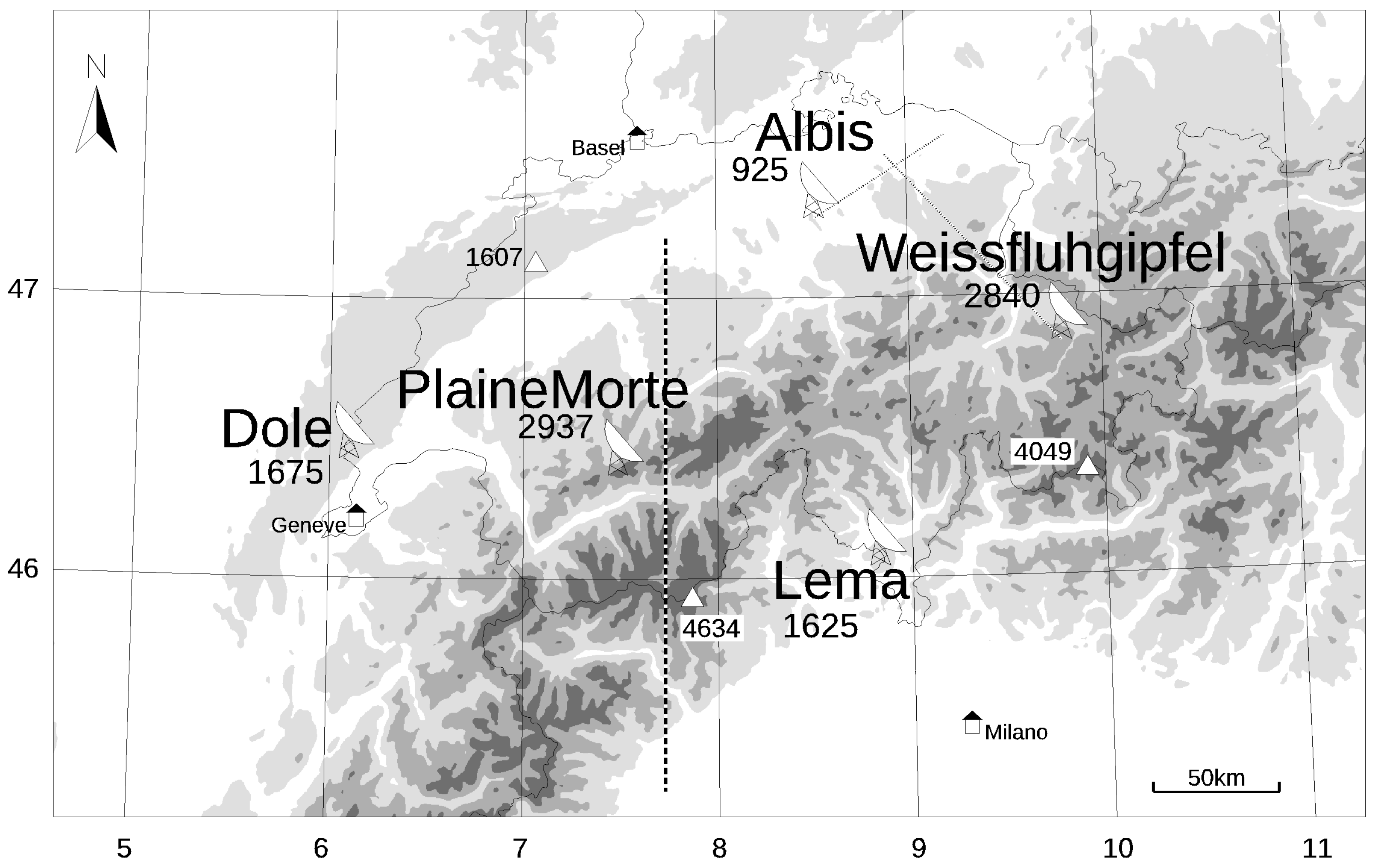
2.1. The Scales of Interest

The temporal and spatial scales of the phenomena at the centre of attention range from a few minutes to several hours, and from a few kilometres to several tens of kilometres. The variability of precipitation at larger scales is well captured by rain and river gauges and by numerical weather prediction models. The principal task of a radar is to capture the spatiotemporal variability of rainfall at small scales, that is, the peaks of precipitation, hail cells and thunderstorms, which are not captured well by point measurements, and to provide the basis for storm severity ranking and warning issuing. Precipitation also exhibits high spatial variability in flat regions, but the regions of maximum rainfall over complex orography are often stationary for a certain period of time, whereas precipitating clouds usually move in flat regions. Because of stationarity, rainfall accumulations can reach extreme values locally, which, in turn, can trigger flash floods, debris flows and landslides. Moreover, a small shift in location over complex orography can make an important difference for the hazards on the ground. A numerical weather prediction (NWP) model can often correctly predict the presence of convective storms. However, it is practically impossible to forecast a thunderstorm at the right location, time and intensity, due to the chaotic nature of convection. An NWP model provides the information necessary to issue a pre-alert that allows people in the affected region to prepare for an event. The level of precision in the location, time and intensity typically required by a user before taking action is so high that it can only be reached shortly before the event, when the presence of a storm is confirmed by the radar. This is the essence of nowcasting, which is primarily based on the latest observations and fast statistical processing. Nowcasting starts with a detailed description of the present weather, such as the quantification of the severity of a thunderstorm, and makes an assessment of the possible hazards. Lagrangian extrapolation of radar fields can help to estimate the location of storms over the following few hours and build the basis necessary to issue a warning. Figure 3 and Figure 4 show the skill and predictable scale as a function of the lead time of a state-of-the-art NWP model and a Lagrangian radar extrapolation nowcast evaluated over the central European Alps against radar observations. The figures show that, in the context of forecasting, a Lagrangian extrapolation of radar precipitation fields provides unique information at a high spatial resolution for lead times of up to a few hours. For a detailed discussion, the reader can refer to [85,86]. According to these results, the crossover lead time, up to which the Lagrangian extrapolation of radar fields has a better skill than NWP forecasts, lies between 2.5 and 3 hours. Interestingly, this result is similar to that found a decade ago for the same study area, but with earlier versions of the models, see [87]. More precisely, the crossover point depends on various factors, and in particular on the type of precipitation and the spatial scale [59].

2.2. Operational Applications in the Swiss Alps

Radar data have been used operationally in the Swiss Alps for quantitative precipitation estimation, which is commonly referred to as QPE [3,4,89,90,91,92], for the nowcasting of precipitation [56,59,62,87], for the tracking, severity ranking and nowcasting of thunderstorms [70,93,94,95,96], for the hail monitoring and hail nowcasting [80,97,98], hydrometeor classification [99,100], wind retrieval and mesocyclone detection [101,102,103,104], data assimilation in numerical weather prediction [63,105] and climatological studies [52,53,55,79]. The applications are continuously reviewed and expanded with new algorithms, see, for instance, [88,97,106,107,108]. Radar products and warnings are sent to air traffic control, weather forecasters, the authorities responsible for the intervention in the case of severe weather and flooding, hydrologists [68,109], and to the private and public sectors. The forecaster on duty provides 24/7 support to users for a correct interpretation of the meteorological data and warnings.

The thunderstorm radar tracking algorithm (TRT) [94] automatically tracks thunderstorms and assesses their severity in real time, through a heuristic approach, using volumetric radar data. The thunderstorms are extrapolated forward in time in the direction of their recent movement on the basis of Lagrangian persistence rules, see Figure 5. The uncertainty of the future cell position is estimated from the standard deviation of the motion vectors of the latest three time steps [70]. Warnings have been issued for future thunderstorm positions since 2005. A warning is issued if either the severity of the cell (TRT) or the amount of rainfall (QPE) within the cell exceeds a predefined threshold [62]. These warnings have been provided automatically and operationally to the authorities via dedicated platforms and to the public via the mobile application (app) of MeteoSwiss since 2020 [95]. The complete warning chain from the radar measurement up to the computation of the warnings and their distribution is fully automatic, without any human intervention. In 2021, a total of 906 of these thunderstorm flash warnings were issued throughout the Swiss territory, which has a size of 41,000 km

^{2}

.

Customised solutions have been developed for particularly demanding applications. The automatic heavy precipitation warning systems developed and configured for a variety of locations and users represent prime examples. These include the operation of a trans-Alpine gas pipeline that crosses a steep Alpine slope that is prone to debris flows, the protection of major construction sites in a river tunnel in the city of Basel [7] and at the railway station in Zurich, the protection of the railway service on a bridge that crosses a catchment with frequent flash floods and debris flows in the Grison Alps (Figure 6) and several other similar applications. Radar measurements are the prime source of information in all these examples of customised nowcasting products. These customised systems often act as prototypes, and the algorithms become part of the standard production for all users in a later step.

Figure 7 shows an example of a recently developed dual-polarisation product to identify hydrometeors. The two operational radars at Albis and Weissfluhgipfel observe the same hail cell, but from different directions and at different distances. The figure shows the different hydrometeor types along a vertical cross section, as identified by the two radars using polarimetric information [99,100]. The presence of hail was confirmed through the measurements of a network of automatic hail sensors on the ground deployed in the hail-prone regions in Switzerland. One sensor of a pilot network that was in the centre of the cell detected 425 hail stones in 6 min. The maximum diameter of 3.3 cm that hit the sensor plate matched the maximum expected severe hail size of 4.5 cm estimated by the MESHS radar product for the corresponding 1 km

^{2}

pixel. Both radars provided sufficient information to assess the severity of the thunderstorm thanks to the high vertical resolution of the scan strategy, which is discussed later on in Section 4.6. This demonstrates that, despite the shielding by terrain, one radar can act as backup, should the other be out of operation. Similar plots for a different hail cell and a discussion on the different types of hail data can be found in [75,98]. The hydrometeor product could trigger new applications in the future, for instance in the automation of human observations (METAR, SYNOP).

2.3. Radar System Requirements

The requirements for the design of a radar network in a mountainous region are derived from the type of weather, the scales of interest and the applications described above:

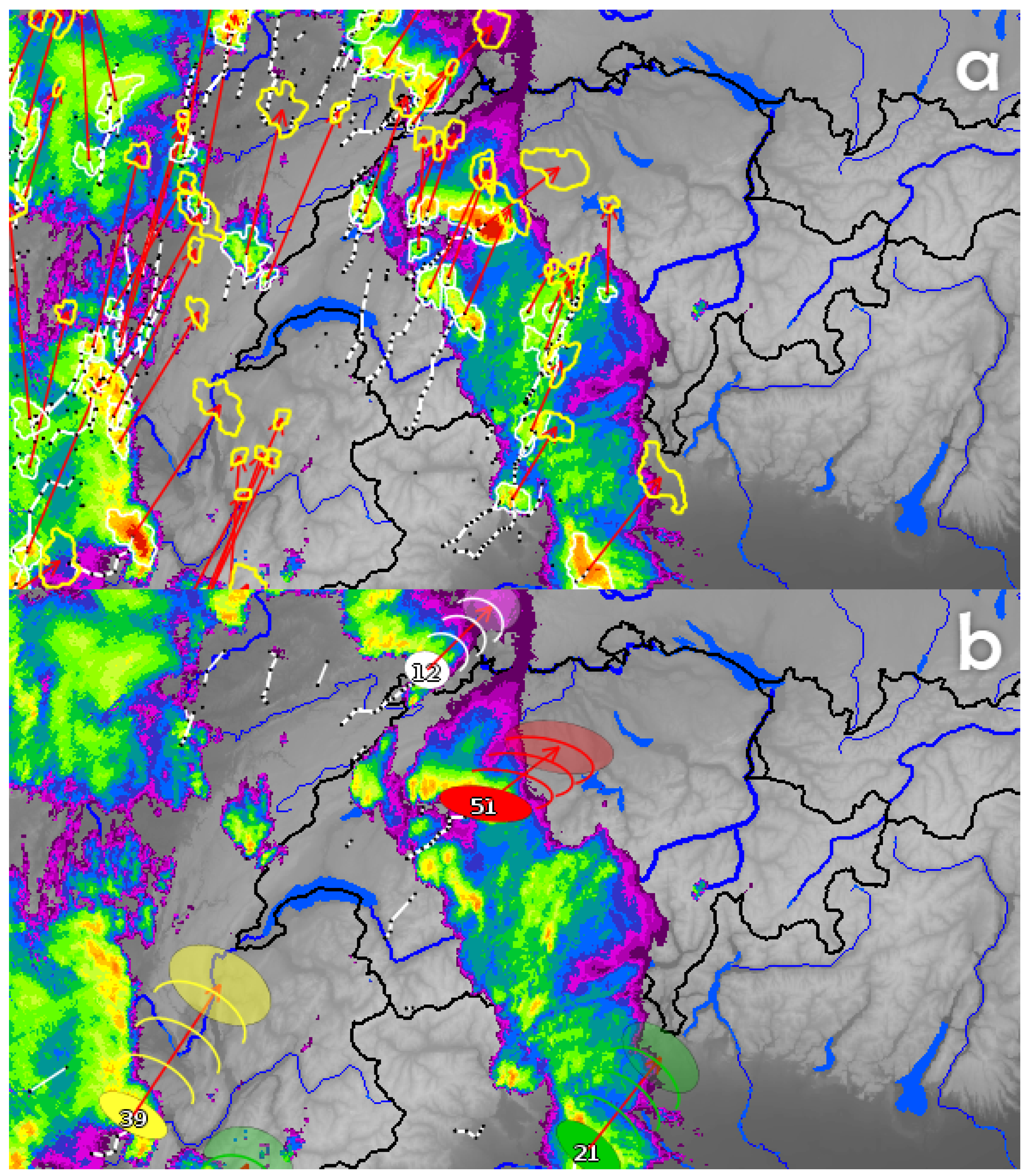
Resolution in time: A high temporal update rate, of the order of a few minutes, is required to capture the rapid evolution of thunderstorms and hail cells, which originate flash floods, debris flows and landslides in steep orography.
Timeliness: Fast data transmission and processing is critical in the context of air traffic control and the issuing of warnings. The radar products have to be ready for submission to the user within about 60 s after the end of a radar volume scan.
Resolution in space: A horizontal mesh size of the order of a kilometre is required to capture rainfall peaks that trigger debris flows, to identify hail pixels inside thunderstorms and to properly describe gradients in thunderstorms and rainfall fields. It is beneficial to have information at scales smaller than 1 km for debris flow warnings and accurate localisation of hail.
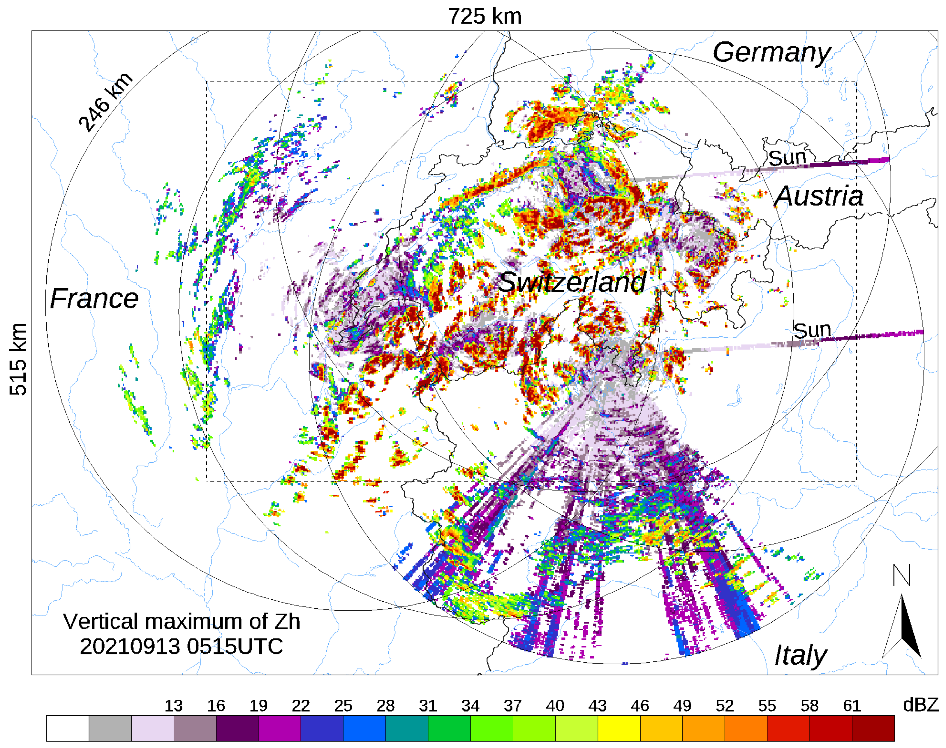
Dynamic range: A network of surveillance radars used for nowcasting has to detect all the different types of precipitation, from weak drizzle to heavy rainfall and hail, for all ranges. This translates into a dynamic range of >100 dB.
Sensitivity: Heavy precipitation and thunderstorms result in high reflectivity values. Therefore, their detection does not put the sensitivity of a radar under pressure. However, sensitivity is critical for other reasons. First, surveillance at long ranges, to see the approaching weather for nowcasting purposes, requires high sensitivity. Second, because of the shielding of the radar beam by the terrain, a substantial part of the measurements in orographic regions are made at a high altitude, that is, in snow, where echoes are weak. These measurements from aloft are then extrapolated to the ground using various techniques. Third, in order to use the Sun for monitoring purposes, the minimum detectable signal (MDS) has to be at least a couple of decibels below the level of the Sun’s signal [110]. If the Sun is also to be used for the absolute calibration of a dual-polarisation receiver, the MDS has to be about 8 dB below the level of the quiet Sun [111]. Indicatively, a surveillance radar must be able to detect echoes down to 10 dBZ at a distance of 200 km.
Stability: Users expect to obtain the same numbers and warning levels in comparable situations. A high stability of the radar hardware is therefore important. One dB is a number that is commonly cited for the stability of reflectivity, and 0.2 dB, which represents an additional challenge, is mentioned for differential reflectivity.
Accuracy and resolution in intensity: Accuracy and resolution are obviously important, but it is not possible to provide one number as a generic answer for reflectivity. The same applies for differential reflectivity, radial wind, the specific differential phase and other radar variables. The question has to be put in the context of a specific application, taking into account all the different types of uncertainties involved in the end-to-end chain and also considering the sensitivity of the application to errors. The cost-loss ratio is one of many ways of doing this.
Information on uncertainties: In modern automatic quantitative applications, it is common practice to take into account information about the uncertainty of the radar product. This is a broad issue, and the requirement depends on the application. For instance, radar rainfall maps and nowcasts need to come as ensembles for hydrological runoff modelling in steep Alpine catchments, in order to deal appropriately with the uncertainties and their space-time covariances in the hydrological model.
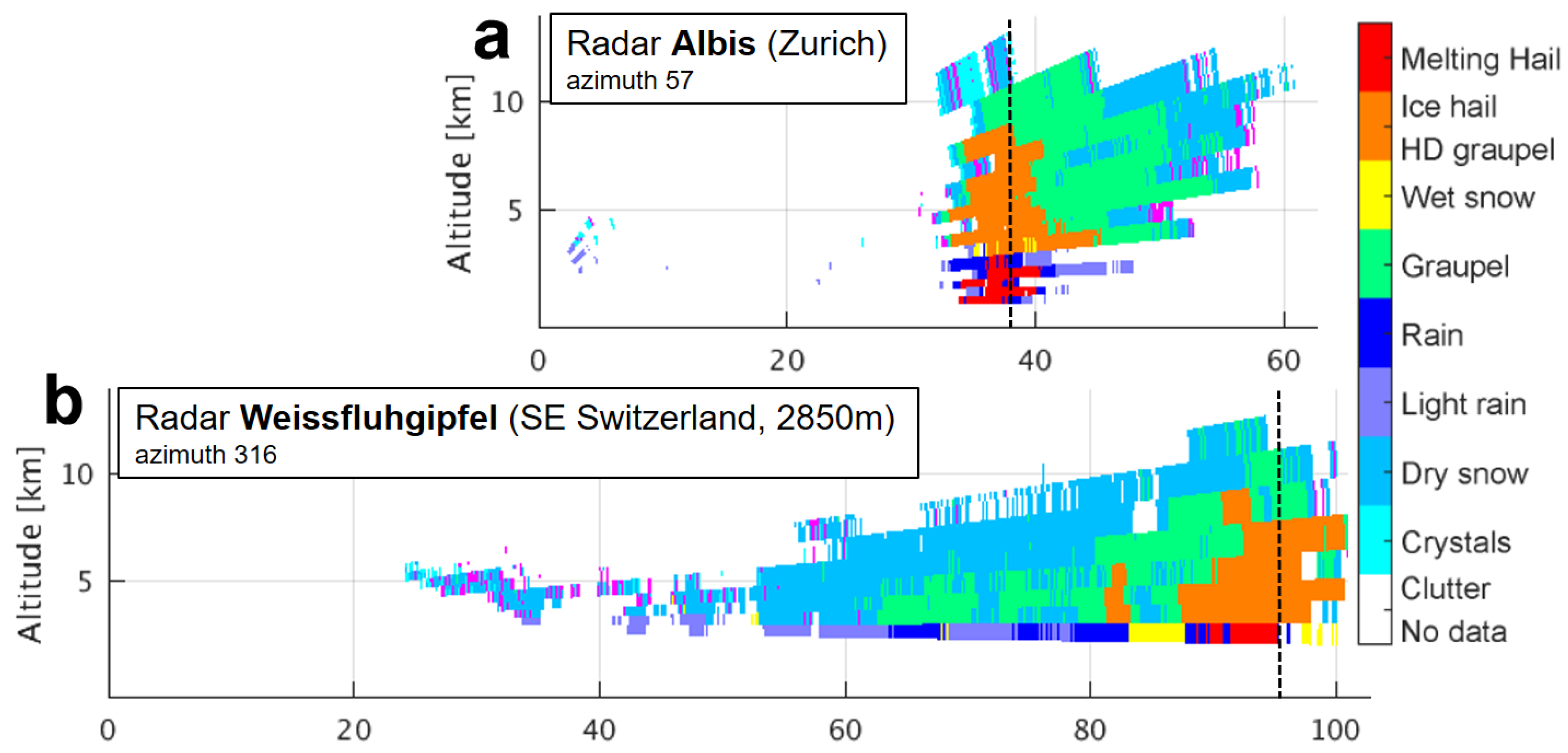
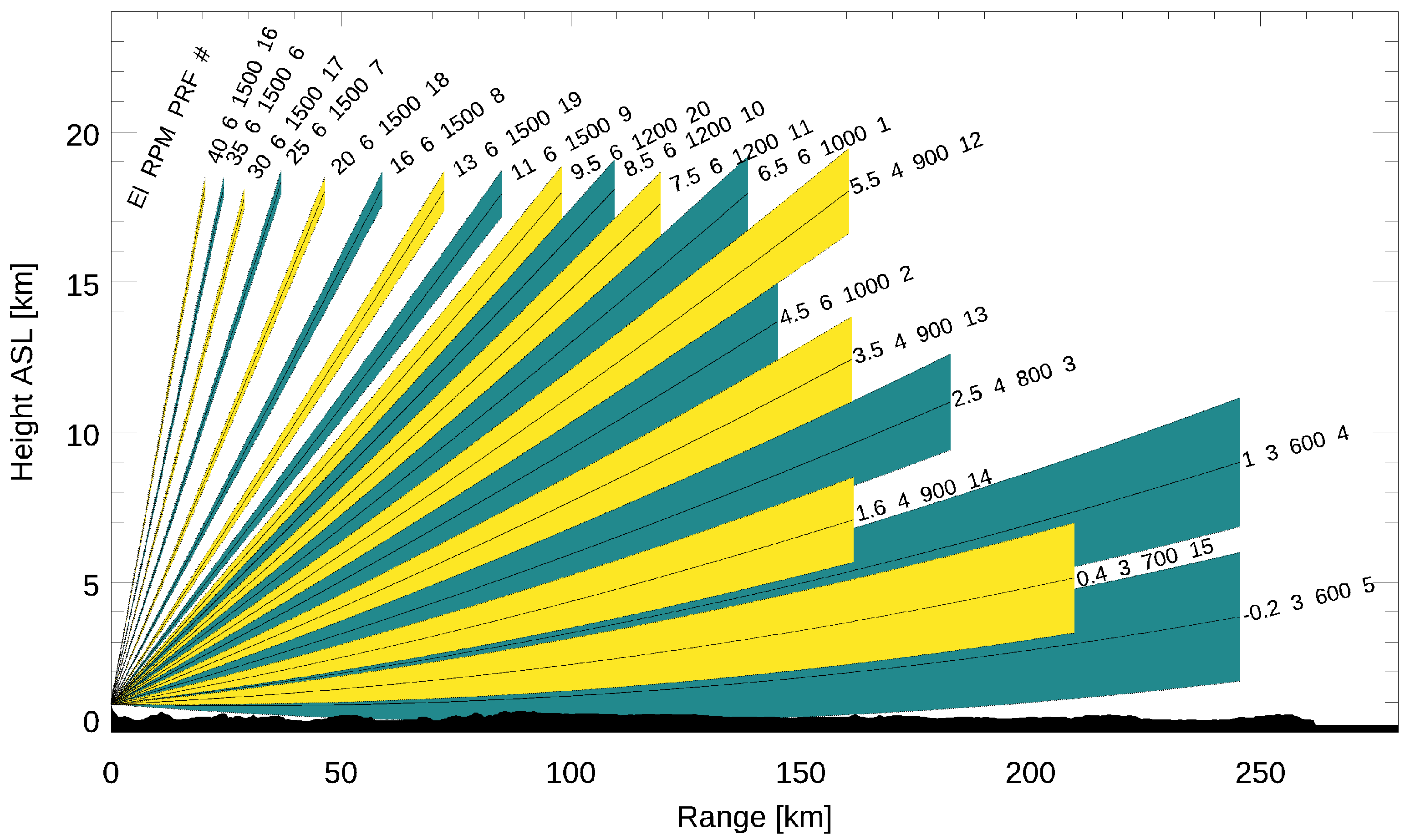
Vertical scanning: It is essential, for the severity ranking of thunderstorms and the identification of hail, to scan from the ground up to the top of the troposphere with a sufficiently high vertical resolution. Small increments of the elevation angle between successive scans at the lowest sweeps help to improve quantitative precipitation estimates over complex terrain.
Continuity: The user expects a certain degree of spatiotemporal continuity in radar products. Sharp artificial discontinuities and artefacts irritate users and may lead to errors in the algorithms that use radar data as input.
Availability: On the basis of the users’ requirements, radar operators typically aim at an availability of radar data above 99%.
Traceability: It is important, in the context of warnings and air traffic control, to record any changes in hardware, software and configuration, to document maintenance work, to archive all calibration values and hardware status parameters and to use calibrated maintenance tools.
Product redundancy: It is necessary to run different algorithms in parallel for the same type of product to cope with the weaknesses of a single method and to have redundancy when one of the algorithms is upgraded or does not perform well for various reasons. Dual-polarisation QPE approaches, for instance, result in a higher accuracy, but are more sensitive to small hardware instabilities than a single-polarisation algorithm. It is therefore recommended to run both in parallel.
Innovation and verification: Both are essential to be able to satisfy the continuously increasing demands of the users.

The information given here corresponds to the situation in the European Alps but can be different in other mountainous regions. The requirements are considered as guidelines for the design, operation and innovation activities of a radar network.

3. Challenges

A large amount of literature is available on the challenges of radar measurement and sources of error in general, see [112] for an overview. For the most part, these also apply to mountainous regions. However, there are three categories of challenges that are specific to the usage of radars in a mountainous region.

3.1. Planning and Installation

The first is related to planning and installation. The choice of a suitable site in itself is often not trivial. The radar has to be high enough to limit shielding and have good visibility over the area of interest, but as low as possible to observe the weather close to the terrain. Long access routes to remote radar sites on mountains and harsh weather conditions pose many engineering problems for the construction of buildings, the installation of the radar, the protection of the infrastructure from hazards caused by lightning, icing, wind and snow storms, and the provision of electricity and data lines. The time window that is suitable for civil work in the summer is often short, and, in the absence of a road, people and the necessary materials must be transported by cable and helicopter.

3.2. Maintenance and Operation

The second category of challenges specific to mountainous regions concerns operation and maintenance. In most cases, radar sites on mountains are unmanned, and access is not guaranteed all year round. Automatic monitoring and the remote control of both the radar hardware and building technology are mandatory. The possibility of monitoring several components of the transmitter, antenna system, receiver, heating, ventilation, door lock status and house climate allows for the early detection of errors and appropriate preparation measures prior to a maintenance trip to the site. It is good practice to have maintenance tools, measurement equipment and a stock of spare parts on site.

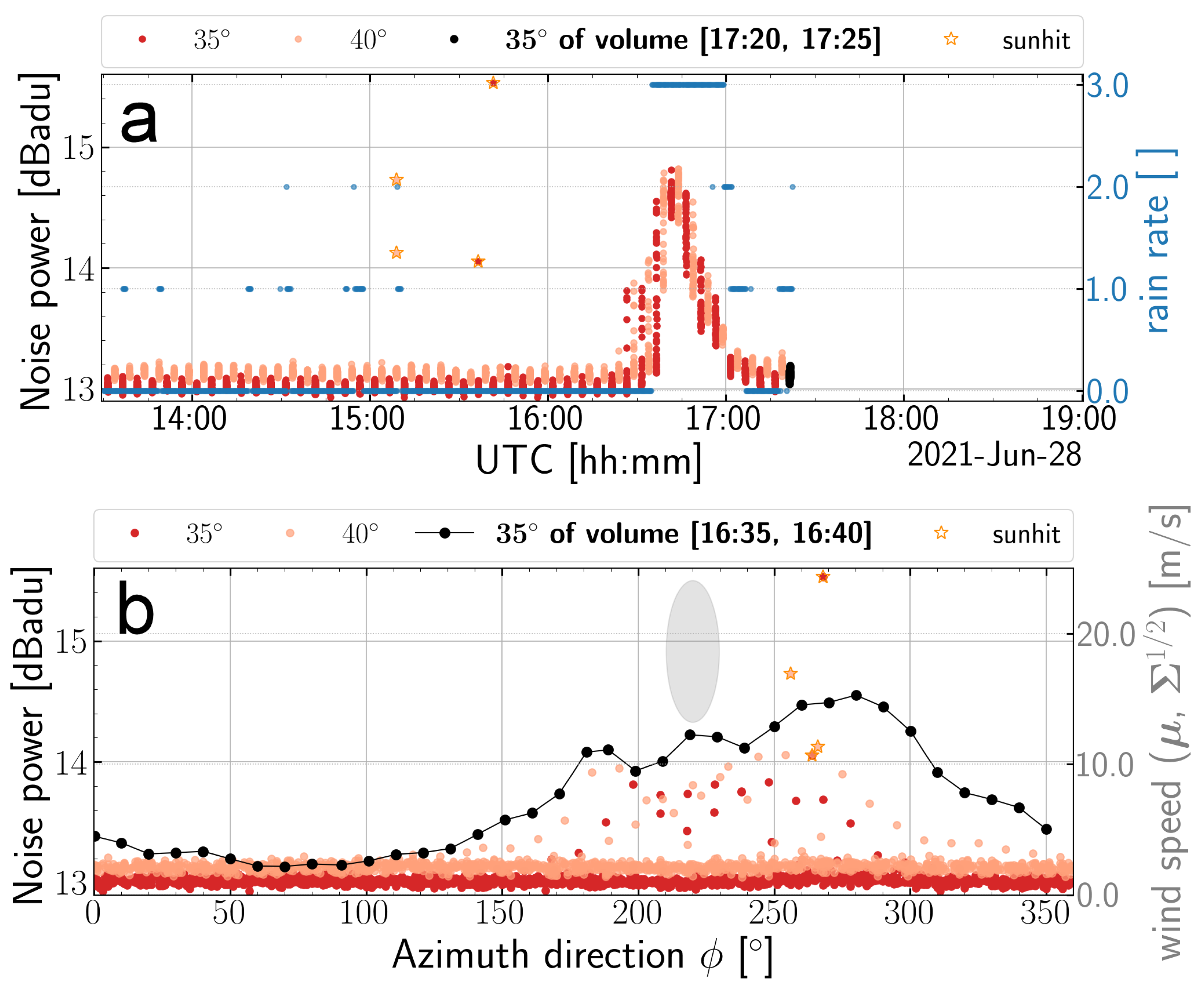
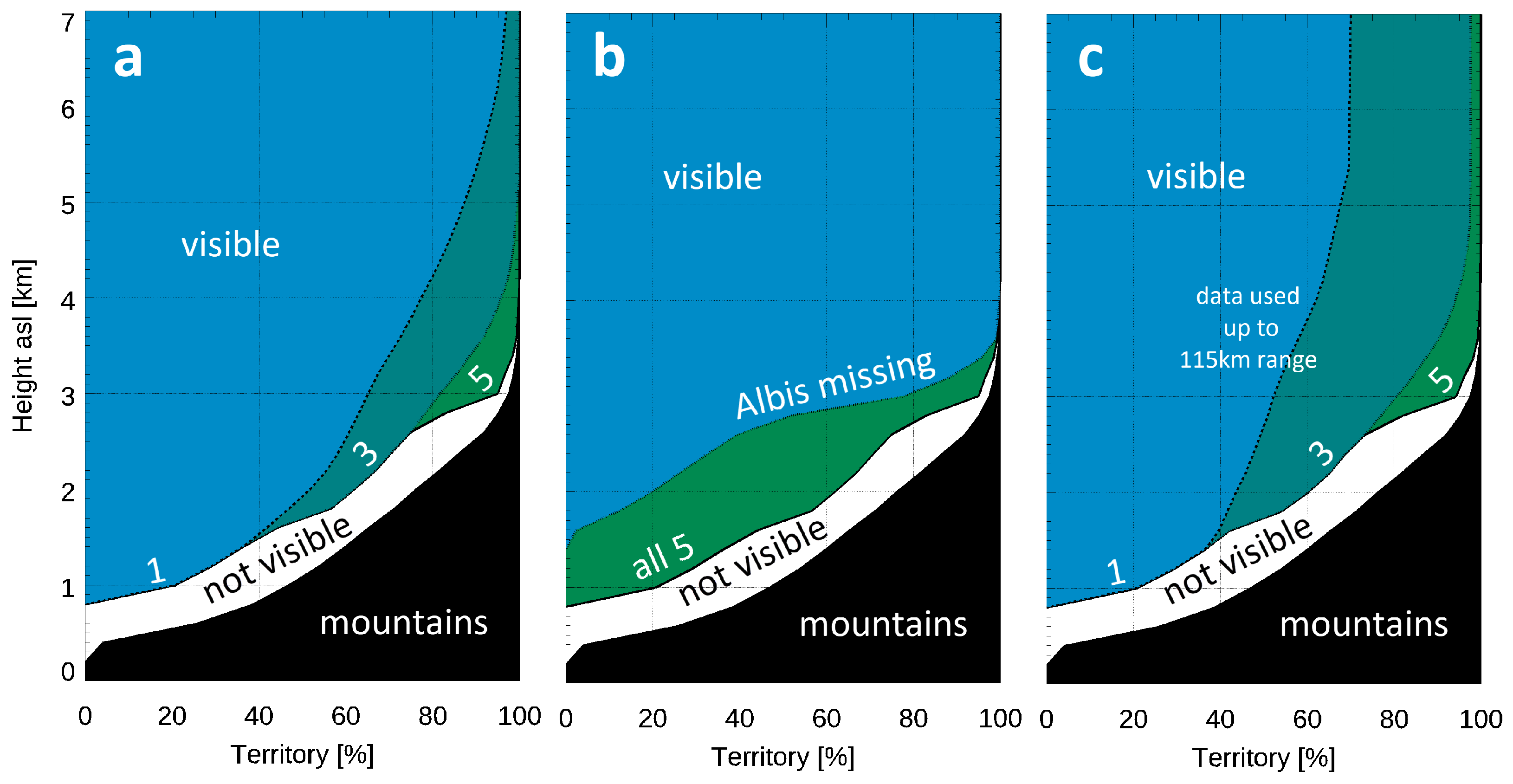
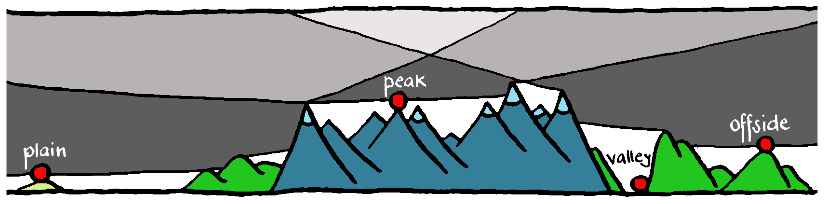
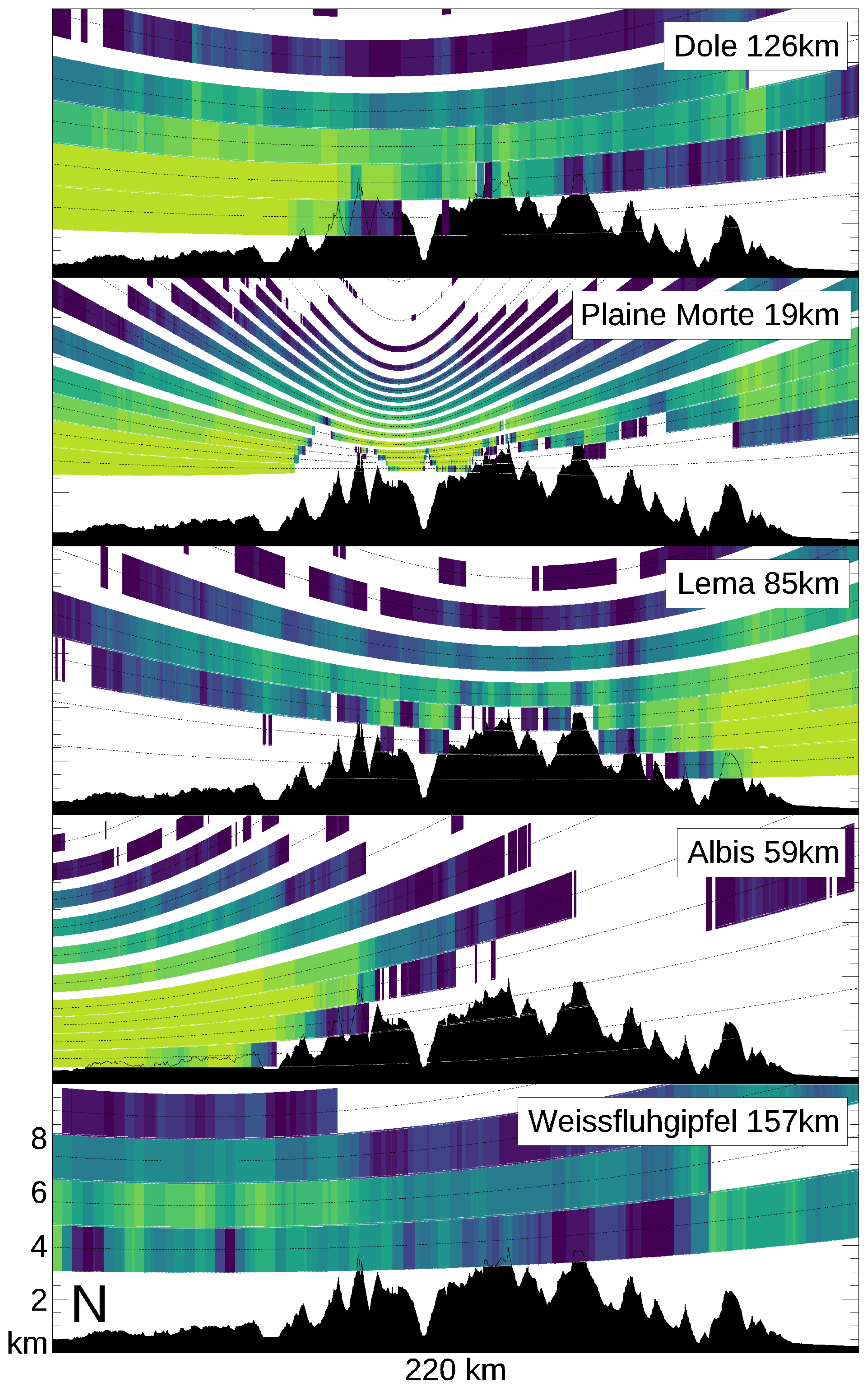
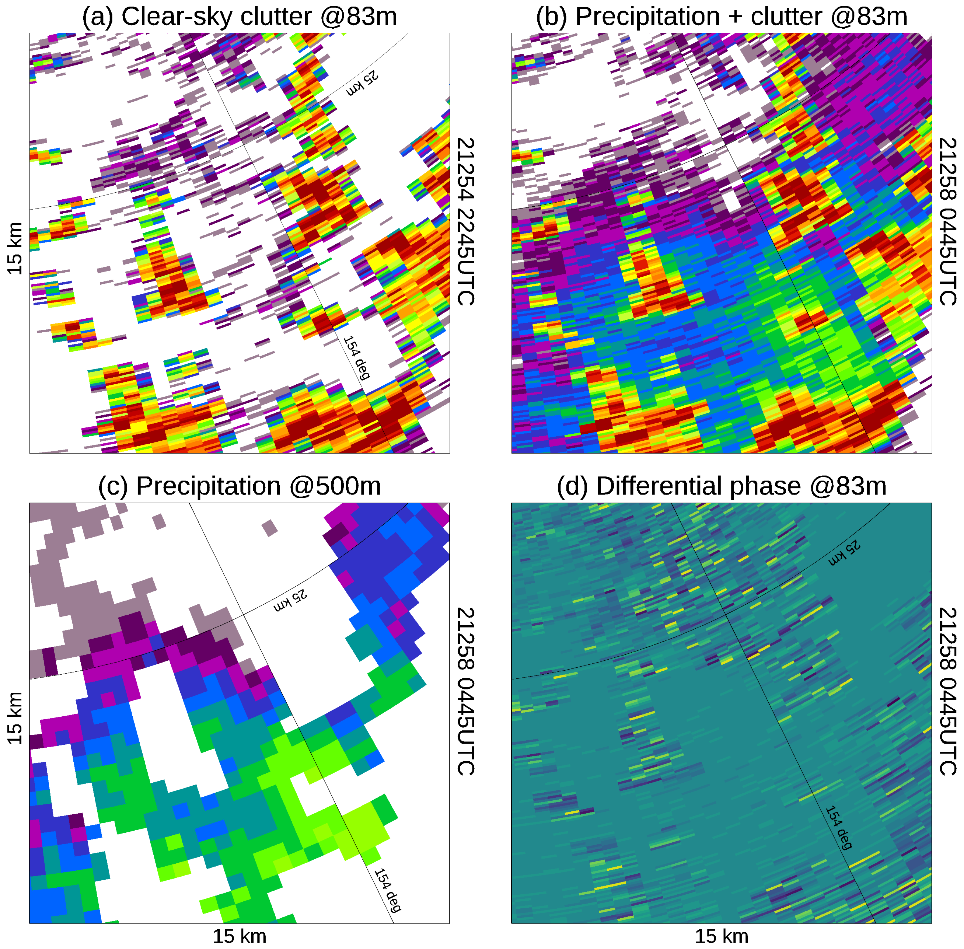
3.3. Reflection and Shielding by the Terrain

Whereas the first two challenges are related to structural engineering and logistics, the third one has to do with the interaction between the radar signal and the mountains. The two most serious problems in this category are (i) the strong reflection (ground clutter) and (ii) the shielding of the radar beam by mountains. Ground clutter is only an issue in a flat region in the vicinity of the radar, up to a distance of about 10 to 20 km. Ground clutter can also occur at longer ranges under certain atmospheric conditions due to abnormal refraction of the beam towards the ground, which is called anomalous propagation, or anaprop. However, ground clutter occurs practically at all times, all ranges and all azimuth angles in a mountainous region, see Figure 8. It is sufficient that a part of the main lobe or any side lobe of the antenna radiation pattern hits the ground somewhere, see, for instance, [113,114]. The amplitude of the signals reflected by the ground is comparable with that of a thunderstorm, and a patch of ground clutter can easily provoke an erroneous automatic thunderstorm, hail or heavy rainfall warning. A rigorous cancellation of ground clutter is therefore essential. The task is particularly difficult when mountain returns are embedded in echoes from precipitation. Simulation studies have shown that dual-polarisation parameters are more sensitive to sidelobe contamination than single-polarisation reflectivity measurements [115]. Applications that build on dual-polarisation measurements thus put higher demands on clutter cancellation, and automatic data quality control in general.

In Figure 8, it is possible to distinguish several different types of cluttered signals. Ground returns are particularly strong and relatively constant in time where the main lobe hits steep mountain slopes and crests, as can be seen from the many yellow-orange-to-red spots within the Alps. The returns from hilly terrain are somewhat weaker and more continuous in space, as pointed out by the violet-blue-to-green areas over France and Italy. Several radial rays can be observed, two of which correspond to signals from the Sun, which was located to the east at the time of this image, while the others refer to signals from external emitters, such as RLAN links. The image also contains ground returns from the side lobes, and possibly a small number of echoes from birds, insects and aeroplanes, which are usually more variable in time but cannot be distinguished with the naked eye in this image.

Another severe problem is shielding of the radar beam by mountains. If only a part of the main lobe is shielded, which is referred to as partial shielding, echoes still arrive from the weather behind the mountain as a result of the remaining part of the beam. The loss of power can be corrected if a fairly good estimate of the degree of shielding is available [3,4,116,117]. Some parameters, such as Doppler velocity and the specific differential phase K

_{D P}

, a polarimetric moment, are immune to partial shielding (and also to calibration errors and attenuation), see, for instance, [118]. This can be exploited for rainfall estimation purposes [119,120,121]. If the beam is completely shielded, the ray behind the mountain will be free of echoes, but the signals sampled by the receiver can be used to study receiver noise and thermal emissions from the terrain, as well as from drops in the atmosphere and water on the radome. The analysis of the signal emitted from water on the radome and in the atmosphere may be used for attenuation correction purposes [122], a concept that needs to be further developed before it can be used routinely in a mountainous region. Figure 9 shows, for illustration purposes, how the noise floor increases when a heavy thunderstorm cell moves over the Albis radar site.

If a beam is completely shielded, it is necessary to rely on the next higher beam to obtain information about any precipitating clouds behind the obstacle. The lower beams in mountainous regions are often shielded, and the radar can only “see” the precipitating cloud starting at heights of some kilometres. Figure 10 shows the present situation in Switzerland with its five operational radars. The intensity of radar echoes decreases rapidly with height, due to phase changes and other microphysical processes, which is commonly referred to as the vertical profile of reflectivity, or VPR in short. The further a measurement is from the ground, the more it becomes difficult to derive useful meteorological parameters, such as the rainfall rates on the ground, and the higher the risk of the radar completely missing a precipitating cloud, which is referred to as overshooting. Overshooting is particularly a problem in stratiform precipitation and generally in winter, when the concentration of scattering hydrometeors decreases rapidly with height. If clutter is adequately eliminated, shielding, combined with VPR effects, are likely the dominant sources of uncertainty in quantitative estimates of precipitation (QPE) in a mountainous region [2,4,89,116,123]. The influence of clutter and VPR effects is less pronounced in a flat region, and other sources of error, such as the space-time variability of the drop size distribution, move into the focus of QPE processing, see, for instance, [124]. The impact of shielding is less critical for nowcasting and the issuing of automatic warnings of thunderstorms because convective storms can arrive well above the height of the lowest visible beam, even when data from one radar are missing (see Figure 10b).

3.4. Other Challenges

The variable of interest in the context of hydroelectric power production, water resource management and studies on the mass balance of glaciers in the Alps, is often the snow water equivalent [125,126]. The conversion of radar signals from snowflakes and ice crystals into values of the snow water equivalent on the ground is another major source of uncertainty, thus adding to the complexity of radar usage over mountainous regions.

Moreover, there are other problems in mountains. It frequently occurs that a radar is at the same height as the melting layer of a precipitation system. This obviously depends on the climate and the height of the radar. In these cases, the radome, the protection sphere around the antenna, will likely be wet and the radar beams at low elevation angles will travel back and forth for many kilometres through melting snow. Both the water on the radome [127,128,129] and the melting snow along the propagation path [12,13] can result in significant attenuation of the radar signal.

4. Solutions and Results

There is no perfect solution for the use of radars in complex orography. Many compromises have to be made concerning the choice of the radar site, the design and configuration of the hardware and the algorithms used for data processing and product generation. If an idea is based on a scientific foundation, has been successfully implemented, has proven to work 24/7 and satisfies the needs of the users, in terms of quality, availability and timeliness, we can call it a “solution”. Ideally, its value is continuously quantified using objective performance indicators, such as statistics of the timeliness, the availability of radar data and accuracy, see Table 1, Table 2 and Table 3. This section presents certain selected examples of solutions, some major performance indicators, the results of recent innovation projects and new research paths. However, the presentation is not exhaustive. It is a selection of aspects that are relevant in a mountainous region and which have a direct link to the practical needs and requirements listed in Section 2.

4.1. Design Considerations

A number of important decisions have to be made at an early stage when the overall design of a radar network over complex orography is necessary. A first important question is related to network design. Do we opt for (i) a dense network of short-range X-band radars deployed on both mountains and within the valleys, (ii) a limited number of long-range C-band or S-band radars sited on mountain crests or (iii) a combination of the two? After careful consideration of all the pros and cons, Switzerland decided to use long-range volume-scanning C-band radars with identical hardware for all of their five sites. However, in a country which has different types of terrain, different sizes, climate and needs, the weather service may opt for another solution. The design of a network also depends on the presence of other observational data, in particular rain and river gauges and satellite imagery, and on the strategy of how these different sources of information will be combined to fulfil the needs of the users.

Another important issue is the design of the data flow and processing stages. Because of the increased bandwidth, it is possible to transmit the radar measurements at an early processing stage from the mountain site to the central computing and compositing server. This allows new sophisticated multiradar approaches to be obtained, for instance, for clutter cancellation and QPE. In the Swiss network, polarimetric moments in polar coordinates are transmitted to the central server at a radial resolution of 83 m. QPE is performed at the central server by combining, for each ground pixel, in a simultaneous manner, raw polar data from all the radars and all the elevation sweeps that provide information on the vertical column above that pixel and for that moment in time. The availability of valid radar precipitation measurements in a vertical column varies considerably in space and time. There are several reasons for this: shielding, ground clutter, variations in the refraction of the radar beam, weather, microphysical processes and the vertical stratification of hydrometeors and, obviously, interruptions of radar operation during preventive and corrective maintenance activities. The more measurements are available in the vertical column above a ground pixel, the higher the quality of the final product. For any given situation, the Swiss QPE algorithms aim to make the best possible combination of all the measurements from different radars and different elevation angles that are available for a given location by assigning different weights to each measurement, depending on the height above sea level, the level of shielding and the distance from the radar. This results in a dynamic and smooth quality transition in space and time, which is a major improvement, compared to the design of the QPE processing of the previous radar generation. The combination of measurements from different elevation angles also compensates for temporal undersampling, which is a major issue when data from only one elevation are considered.

The testing of new algorithms can easily be done offline with historical data sets. However, when evaluating new radar products, together with forecasters and the users of automatic heavy precipitation warnings, it is essential to be able to run new software in real time on a test chain that is identical to the operational chain. There are four parallel real-time processing chains on the central radar server of the Swiss network, two for testing, one for deployment and one for operational production. There is also a second digital signal processing unit on one of the radar sites (Albis) that runs in parallel with the operational one. It is used for testing purposes and as a spare part in the case of failure.

The spatial and temporal resolution of product generation is another important design aspect. In the case of QPE, and most other radar products, the uncertainties are large and it is recommended to integrate values over time and/or space to reduce the stochastic errors. Nevertheless, it is good practice to generate the radar products with a sufficiently high space-time resolution of the order of 1 km and a few minutes, and then to do the integration later, depending on the specific setting of the application. The Cartesian products in Switzerland are generated with a resolution of 1 km and updated every 2.5 min, a reasonable choice, considering the requirements listed in Section 2.

4.2. Siting

The choice of a suitable site is obviously a critical step. Many studies have been presented in the literature to simulate ground clutter and shielding of a radar using digital terrain information and a beam propagation model, see, for instance, [19,113,114,116,130]. Siting in a mountainous region is always a compromise between a high site on a peak in the centre of the mountain range with limited shielding and the possibility of long-range surveillance (we call this type “peak”), a mountain site at an intermediate height on a crest somewhat offset from the main mountain range with the highest peaks (“offside” type), or a site lower down in a valley that allows the precipitating cloud to be observed at low heights (“valley” type), see Figure 11. In addition, there is also the “plain” type, which corresponds to a radar sited on a tower or a hill that is far away from the nearest mountain range and can overlook a plain with few or no obstacles. This subdivision is oversimplified, but it illustrates the main options for siting a radar to oversee precipitation over complex orography. All four types have pros and cons, and none is ideal. A combination is likely to give the best results.

For the “peak” type, it is tempting to chose one of the highest peaks of the mountain range. However, this is probably not the best option. Moving away from the ridge with the highest peaks, it is often possible to find a considerably lower site with limited shielding, better access, easier conditions for construction work and the possibility of seeing the precipitating cloud at lower heights. The latter is an important aspect, as the number of hydrometeors and the chances of obtaining a sufficient number of good measurements, which would allow meteorological variables to be derived, decreases rapidly with height, see Section 3. A radar of the “peak” type can not see down into narrow valleys, but it is the only site in complex orography that allows precipitating clouds to be sampled close to the terrain and with a narrow beam over a large area. The beams of the radars of the “offside” and “plain” types over the mountain range are high above the terrain and broad, due to the long distances. A site of the “valley” type can see falling hydrometeors down in the valley, but its range is seriously limited by the surrounding slopes and crests.

The Swiss radar sites on Monte Lema and La Dole belong to the “offside” type, whereas the two Alpine sites on Plaine Morte and Weissfluhgipfel, which were added in 2014 and 2016, are of the “peak” type (Figure 1). Another example of the “peak” type is the Austrian radar on the Valluga mountain. The site of the polarimetric Doppler X-band radar, operated by the University of Grenoble, see, for instance, [131], is an important example of the “valley” type with ideal visibility over the target area, that is the city of Grenoble. The sites in deep Alpine valleys of the mobile polarimetric X-band radars operated by EPFL and MeteoSwiss also belong to the “valley” type, see, for instance, [132]. The radars on Albis near Zurich and Bric della Croce near Turin (Italy) are examples of the “plain” type.

Figure 12 illustrates the contribution of different types of sites to the observation of precipitating clouds over and near a mountain range. It shows precipitation accumulated over one year (2016) along a vertical north–south cross section that crosses the central European Alps. However, there is no single ideal site. Only a combination of different types of sites in complex orography will provide good data quality in all regions. Data quality decreases as the range and level of shielding increase. Nevertheless, a radar far away from a point of interest can still provide data of sufficient quality whenever the prime radar for that location is out of service. This is part of a strategy to obtain high availability of radar data in an operational setting.

4.3. Installation, Acceptance Testing and Lightning Protection

The installation work of the Swiss radars had to be supported, to a great extent, by helicopters. Before starting the challenging civil work to install a new radar on a remote mountain peak, it is good practice to conduct detailed tests at the factory. Testing and fixing technical problems is far easier in a factory than at 3000 m above sea level. The Swiss radars were thoroughly tested on the roof of the supplier’s factory as part of the formal acceptance process by analysing data injected by test equipment, reflections from a nearby tower, signals from the Sun, and echoes from precipitation, while operating the radar in the foreseen operational configuration. During the factory tests, which lasted several weeks, the hardware monitoring parameters were recorded in real time and various aspects were analysed.

Another novel element for acceptance testing was a 6-month test period in operational mode, which started upon completion of the site acceptance test at the end of commissioning. The 6-month operational test was followed by a final 4-month test of the whole network. Throughout the acceptance testing, the combination of different pieces of complementary equipment and sources of information proved to be a good strategy. In addition to standard tests, MeteoSwiss deployed an external receiver and an external transponder, and implemented numerous experiments to gain as much information about technical and functional performance of the radar as possible. The transponder can introduce a time delay, which allows the signal to be moved to a silent gate, with no clutter contamination. It can also add a shift to the Doppler frequency and change the polarisation, which are interesting options to make independent measurements of the specifications of a new radar [133].

Protection from lightning is another aspect that needs to be carefully thought through for radars on exposed mountain sites. A direct lightning strike can cause major damage to the radome [134] and the antenna, the repair of which could take several months. The damage caused by indirect lightning currents, which enter via the power or data line, is generally less serious, but locating and fixing the damage can be lengthy and complicated. Adequate protection from lightning is thus mandatory. On the other hand, it is desirable to avoid, as much as possible, any interference of lightning protection rods around the radome on the radar measurements. It has been shown that lightning poles can cause significant interference, in particular for polarimetric moments. Two groups of rods have been used to protect the Swiss radars from lightning, one is situated below the lowest point of the antenna, and the other one is located in the upper part of the radome, see Figure 13. With this design, the risk of interference is marginal and limited to the highest sweeps, which are less critical for quantitative rainfall estimation. To date, no interference has been witnessed in the measurements.

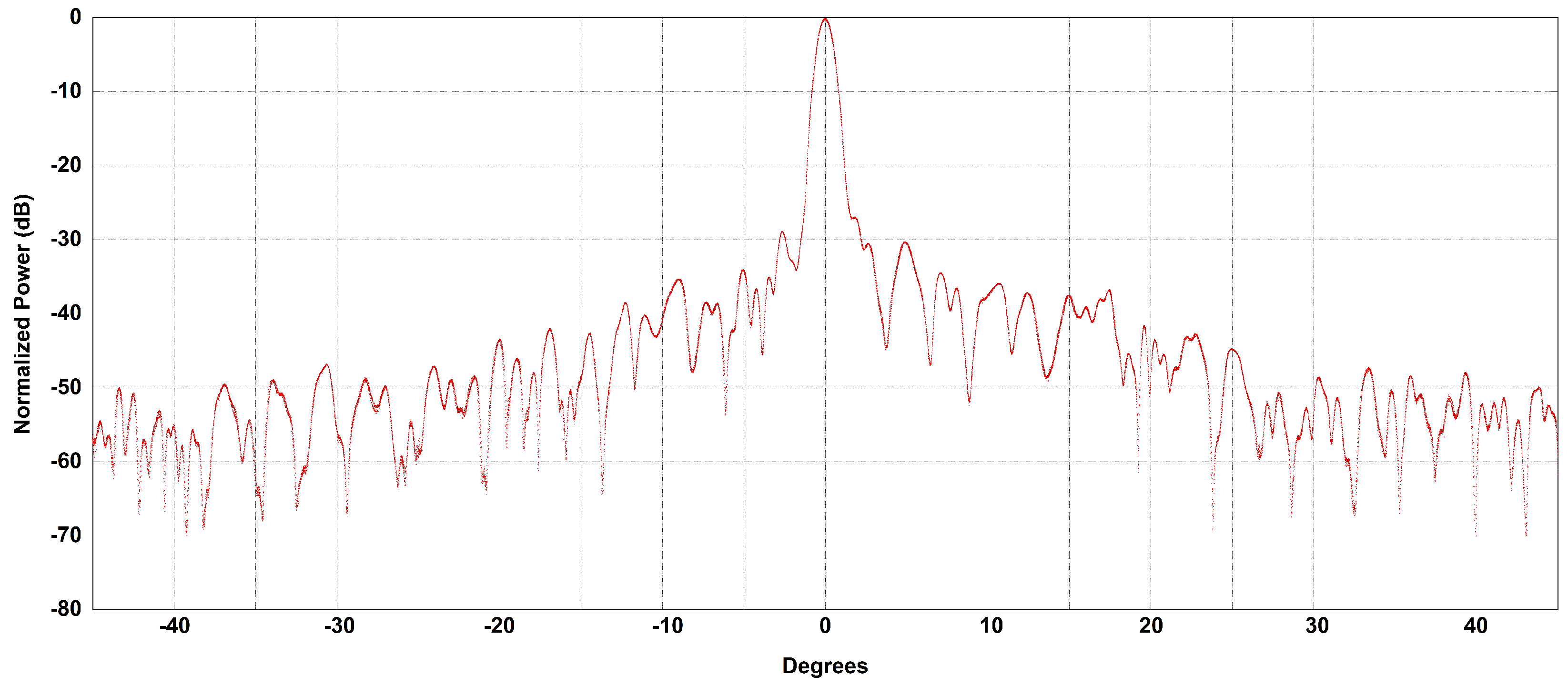
4.4. Radio Frequency and Polarimetry

The choice of the radar hardware and configuration is driven by the needs and requirements of the practical applications (Section 2). For a mountainous site of the “peak” or “offside” type (Section 4.2 and Figure 11 and Figure 13), limited space, difficult terrain for civil work, harsh weather and the budget lead to an upper limit on the size of the building, the radome and thus also of the antenna. For a given antenna size, shorter wavelengths result in a higher antenna gain, a narrower beam, lower sidelobes and a more favourable ratio between weather and mountain returns (clutter) [1,2]. Gain, beam width, sidelobes and the weather-to-clutter ratio are all critical aspects for operational radars in complex orography. On the other hand, the shorter wavelengths of X-band radars and, to a certain extent, also C-band radars, suffer from signal attenuation as a result of water on the radome and of large rain drops, melting snow and melting hail along the propagation path, whereas attenuation can largely be neglected for S-band radars, except for hail. The choice of the wavelength should be a compromise between the above counteracting arguments. Complex orography countries often opt for C-band radars for volume-scanning surveillance [1,8,37] and X-band radars for research and field campaigns [135], gap-filling [9,126,136] and urban hydrology [131].

X-band radars in complex terrain are sometimes promoted because of their low costs and high spatial resolution. However, this is a little misleading. The low costs are mainly the result of the small overall size of the X-band system, which has typical antenna diameters of between 1 and 2.5 m. However, the resulting beam width of these antenna diameters is comparable with or even broader than that of a C-band radar with a 4-m antenna. The advantage in the spatial resolution that can be achieved with X-band wavelengths is lost if a small antenna is used to limit the overall size and costs.

Many of the radar measurements in a mountainous region are made in solid precipitation and the applications of polarimetry, based on the axis ratio of drops, are limited to the measurements that are made below the melting layer. Furthermore, polarimetric moments are more sensitive to contamination from ground clutter from the main and the side lobes [121] and, in the case of differential reflectivity Z

_{D R}

, to calibration errors and hardware instabilities in the transmission and reception paths. In spite of this, dual polarisation produces a large benefit in complex orography as it offers a better distinction between weather echoes and ground clutter (Section 4.10), and it can be used to obtain information on the type and mixing of hydrometeors (Figure 7 and [99,100]), to diagnose hardware anomalies, to correct signal attenuation and to improve quantitative estimates of the precipitation rates (Section 4.10). Last but not least, the vertical channel (V) can be used as a backup for single-polarisation algorithms whenever the horizontal channel (H) suffers from instabilities. The extra costs of dual polarisation are modest and the gain in quality and quantity of information is large, but a robust solution for the calibration and monitoring of both channels is critical [137].

4.5. Receiver over Elevation Design

Some countries opt for a design with the receiver mounted onto the back of the antenna, that is, the so-called receiver over elevation design, or short ROEL [137,138]. Some examples of this type are the Italian radar on Bric della Croce [15,139], a hill near Turin, and the operational networks in Austria [8], Belgium, Germany [140] and Switzerland [1]. For a picture of the receiver over elevation design, see [5]. A ROEL design offers several advantages:

The reception path is short, which results in improved sensitivity;
On transmission, the same waveguide and the same rotary joint are used for both the horizontal (H) and vertical (V) polarisations up to the power divider (magic-T) on the back of the antenna, which results in higher accuracy for dual-polarisation moments;
The transmission and reception paths are symmetric for H and V polarisation;
There is no need for an expensive (and sometimes fragile) dual-channel rotary joint.

Measurements conducted during commissioning of the new radar at Albis [1] pointed out that the sensitivity had improved by 9 dB, a number that was roughly confirmed by means of Sun measurements. Part of the gain in sensitivity at Albis can be attributed to switching to the ROEL design, while the rest can be attributed to the replacement of the analog receiver with digital technology and moving the transmitter and receiver from the cabin at the bottom of the tower to the top. Sensitivity is a critical aspect for radars in complex orography, as stated in Section 2. In spite of obvious advantages, ROEL does not seem to be the preferred option. The majority of national weather services prefer a conventional design with the receiver next to the transmitter in the cabin. A possible reason for this may be the need for a reliable broadband data line between the receiver on the moving antenna and the cabin, which can be realised, for instance, with a fibre optic line in the centre of the rotary joint [138]. Other reasons may be related to the need for a reliable control of the climate in the receiver box and appropriate lightning protection in the radome. Another frequently cited counterargument is that of the significant additional efforts that are needed for maintenance work, but this has not been confirmed for the Swiss experience. A ROEL design is difficult to realise for an S-band radar for technical reasons, because of the large size of the waveguides. For more specifications on Swiss radar hardware, see Table 9.1 on page 175 in [1].

4.6. Scanning the Atmosphere over Complex Orography

The quality of radar products in complex orography depends to a great extent on the way the antenna scans the atmosphere, which is commonly referred to as the antenna scan strategy. This is part of the radar configuration and determines:

The total number of sweeps in a volume scan, which is important for a thunderstorm severity estimation, hail identification, QPE, hydrometeor classification, mesocyclone detection and wind retrieval;
The number of sweeps and angular overlappings at low heights close to the terrain, a critical aspect for QPE processing;
The number of independent measurements per ray, which determines the precision of an individual measurement;
The maximum height up to which echoes are sampled, which is relevant for the estimation of the echo top, VIL, the wind profile, thunderstorm severity and hail identification;
The conical volume above the radar, where no measurements are made (the so-called cone of silence);
The total time required to complete a volume scan, a critical parameter in the context of air traffic control, nowcasting and issuing automatic warnings;
The pulse repetition frequency, PRF, which determines, in opposite directions, the maximum unambiguous range and the Nyquist interval. The latter has an impact on wind retrieval and mesocyclone detection;
The diversity in the Nyquist velocity between neighbouring sweeps, which helps in de-aliasing;
The order of the sweeps: for instance, an interleaved approach reduces the effects of temporal undersampling of rapidly evolving storms.

The scan strategy of the networks in the Austrian and Swiss Alps are both characterised by a comparatively large number of sweeps (16 and 20, respectively), which are sampled in an interleaved scheme, and completed in a short time (5 min), see Figure 14 and [1,8]. As a result of the high elevation angles, the cone of silence above the radar is relatively small. These configurations were driven by the above considerations and the needs and requirements discussed in Section 2. The interleaved scan leads to zigzag patterns in the vertical cross section in rapidly evolving storms, see, for instance, the melting hail signature in Figure 7. Zigzagging is an artefact that is caused by the rapid evolution of a storm during the time the antenna takes to complete half of the volume scan. A zigzag pattern is apparently a disadvantage, but in reality, it conveys more information about the evolving storm than an identical scan without the interleaved scheme. Cartesian radar products in Austria and Switzerland are generated every 2.5 min, combine the two most recent half-volume scans, and hence take advantage of the interleaved approach.

Technically speaking, it is possible to adapt the antenna scan program in a dynamic manner, depending on the type and location of the precipitating clouds. Dynamic scanning allows an increased resolution to be obtained in space and time in a dynamically selected target area, which has weather of particular interest. This may be an interesting option for gap-filling or any research radar that is not strictly necessary for long-range surveillance, see, for instance, [96], or for a network that was designed for dynamic scanning from the start [141]. It is questionable whether the gain in resolution in some selected areas of a long-range surveillance radar in a mountainous region, where precipitation is frequently present in several different azimuth sectors, is worth the extra complication of the configuration, antenna control, data processing and product generation. Moreover, there is the risk of missing precipitation in some locations outside the area of the targeted scanning.

4.7. Pulse Length

Another aspect of complex orography that merits consideration is the choice of the pulse length. Although some sensitivity is lost with a short pulse, it has the great advantage of keeping the area contaminated by clutter small and it is possible to obtain clutter-free measurements of precipitating clouds just before and after the gates where the beam hits the ground. This is illustrated by the reflectivity measurements, at an 83-m radial resolution, obtained with a pulse length of 0.5 microseconds, shown in Figure 15.

Moreover, using short pulses, more independent samples can be obtained to reduce stochastic errors from signal fluctuations. This improves the precision of polar radar measurements. Furthermore, short pulses make it possible to reveal fine-scale signatures, which may be of particular interest in the presence of severe convective storms. These may allow a better assessment to be obtained of the hazards related to supercells, hail cores and local rainfall extremes, a topic of ongoing research at MeteoSwiss and EPFL.

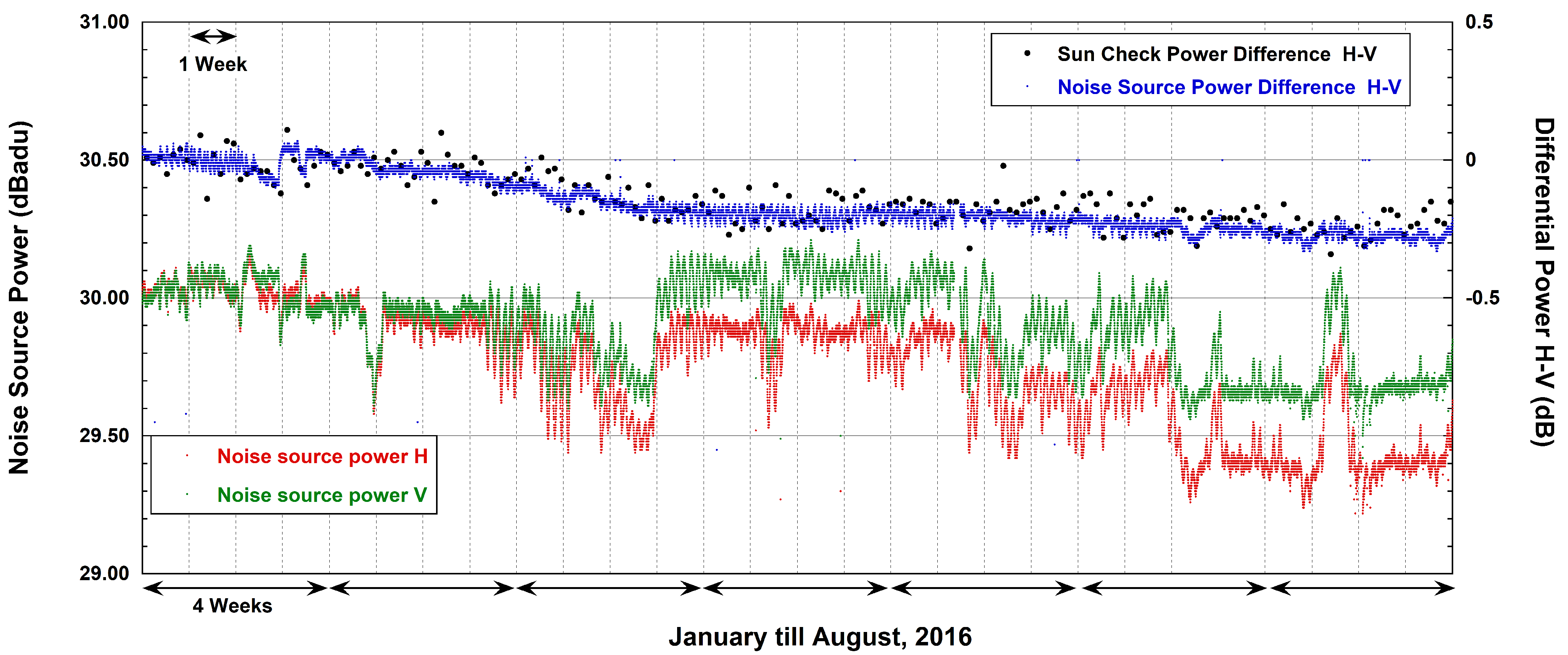
4.8. Calibration, Monitoring and Control

Automatic calibration, comprehensive monitoring and remote control are also important in flat countries, especially if the radar is used for air traffic control, automatic warnings and other demanding applications. However, they are of even greater importance in a mountainous region where there are remote unmanned sites, long access routes and periods when no access is possible. The aim of these procedures is to automatically detect instabilities, ageing components and the risks of failures at an early stage, and to have as many data as possible available to diagnose the origin of a problem. The final goal is to maximise stability and minimise the down time.

Absolute calibration strategies generally combine offline and online procedures. A number of measurements are performed offline at the factory, during commissioning, and are repeated on a regular basis during preventive maintenance operations. These include measurements of the losses along the transmission and reception path, of the characteristics of the transmitted signal (output power at the magnetron, frequency and pulse shape), and of the system dynamics (in particular the minimum discernible signal, alignment of the high-sensitivity and low-sensitivity channels). If changes in the transmitting or receiving path occur, the signal losses need to be remeasured. Ideally, the antenna gain and radiation pattern should also be measured under conditions after commissioning, with and without the radome, but this is difficult, especially in mountainous sites, and is thus rarely done.

If no hardware changes occur, the losses in the receiving path should remain stable. In reality, certain components, such as receiver protection devices (e.g., TR-limiters), can degrade. Moreover, certain components are sensitive to temperature, and their performances thus vary over time. It is therefore good practice to monitor the receiving path online by means of an automatic scheme. In Switzerland, for instance, reception losses are sampled using the signal of a noise source injected every 2.5 min in the H and V reception channels, both before and after the TR-limiter [137]. Atmospheric background noise, which is sensitive to degradations in the receiving path, is also monitored. Absolute calibration is therefore achieved by automatically combining the offline and online measurements and adapting the radar calibration constant of the H and V channel accordingly. This procedure is repeated every 5 min and in this way compensates for temperature dependencies of the receiving path.

The absolute and differential accuracy of the two polarisation channels can also be monitored by means of Sun measurements, obtained online in operational mode, whenever the antenna points in the direction of the Sun [142,143,144] and during dedicated manually triggered Sun scans performed on demand [110,111]. The Sun’s signals detected by the radar receiver are also used to monitor the pointing of the antenna. Another option to monitor the stability of radar measurements is to analyse the signals scattered back by a tower nearby, see, for instance, [145], or by mountains [12,13]. During the renewal of the radar network in Switzerland [1], an external receiver and an external transponder were deployed on a mountain in the vicinity of the radar being tested, which allowed, for instance, the antenna gain, parts of the antenna radiation pattern (Figure 16), the shape of the pulse, the precision of the scan strategy and depolarisation to be examined. At the moment of writing (2021), the external receiver is still in use for monitoring purposes, 10 years after the renewal of the Swiss radar network. A number of additional techniques are available to monitor the stability and accuracy of dual-polarisation moments, see [106,146,147] and references therein.

Overall, the Swiss radar sites each send more than 370 monitoring parameters to the central processing server for every elevation sweep, that is, every 10 to 20 s. These include parameters of all the hardware components (antenna control unit, transmitter, receiver), the temperature and humidity in various locations (outside, inside the radome, in the technical room, inside the receiver box), and the building infrastructure (heating, ventilation, climate, uninterrupted power supply, electric consumption, door lock). The strategy behind this is to monitor a large number of parameters at a high temporal resolution, which are automatically analysed for suspicious trends, discontinuities and other anomalies. All the monitoring parameters are archived and can be accessed manually via an interactive online platform that was designed for system diagnostics and troubleshooting, both remotely and on site, by the maintenance personnel.

Figure 17 shows the degradation of an ageing TR-limiter. The red and green curves show the signals detected by the receiver in silent gates when the noise source was injected in front of the TR-limiter of the horizontal and vertical polarisation channels, respectively. The temporal variation of the red and green curves exhibits the dependence of the receiver channels on temperature. When calculating the difference between the two, a continuous degradation of the horizontal channel was revealed, which, over the course of six months, reached a value of minus 0.3 dB. This degradation is confirmed by the online samples of Sun’s signals and is related to the ageing of a defective TR-limiter. Interestingly, this degradation was not confirmed, to the same extent, by the measurements of repeated manually triggered slow scans of the Sun performed offline at three different stages during the same period (not shown in Figure 17). The manually triggered offline measurements of the Sun revealed a degradation of only minus 0.05 dB, the reason for which was not clear. This illustrates the importance of using different sources of information in parallel for one and the same aspect being tested. A bias in the reflectivity measurements of the order of 0.3 dB is not critical for single-polarisation algorithms, but it can lead to significant errors in products that rely on dual-polarisation data.

In another case, the combination of different information sources was the key to locating the cause of an error. During the acceptance tests of the new dual-polarisation radar on Lema, differential reflectivity Z

_{D R}

was monitored by means of measurements of the Sun, drizzle, an external transponder and an external receiver. The measurements of the Z

_{D R}

bias from the Sun (+0.8 ± 0.1 dB ), drizzle (+0.8 ± 0.2 dB ) and the external transponder (+0.6 dB ) all revealed a bias with the same sign and of the same order of magnitude. However, the test with the external receiver, which is the only one that does not include the receiving path of the weather radar, revealed a small bias, in the opposite direction, of

- 0.1

dB. These test results correctly pointed out an error in the receiving path, and the issue was solved by replacing the Rx calibration unit of the Lema radar.

4.9. Availability and Timeliness

If the radar data are used for air traffic control, severe weather warnings or other safety-related applications, timeliness and availability are crucial. With an appropriate design and implementation of the data transmission and processing chain, the base products, including radar QPE, are ready for submission to the user within about one minute after the completion of a volume scan. The times are somewhat longer for enhanced products, such as thunderstorm nowcasts and heavy precipitation warnings, which also include data from other observation systems (a lightning detection network, rain gauges, satellites) and from the numerical weather prediction model. Table 1 shows timeliness statistics, as retrieved by the automatic real-time monitoring system, for different types of products of the Swiss radar network. The base and enhanced products include both single-radar and composite products of all the five radars.

The antenna takes about ten seconds less than the nominal time to complete a volume scan. This time is enough to transmit and process all the base products, including radar QPE, for 50 percent of the cases, see the 50th percentile in Table 1. For 90 percent of the time, the base products are ready within 8 s (90th percentile), while for 99.95% of the time, they are ready within 60 s (last column). The times could be further reduced, if necessary, by means of parallel processing and a further optimisation of the processing chain. On a few days, and for a limited duration, the data transmission and processing took more than 300 s. These delays are related to planned interruptions of the central processing computer for upgrades and security patches of server hardware, which are scheduled on days in which there is no significant precipitation.

Table 1. Timeliness of products generated every 5 min by the Swiss radar network. Timeliness has been monitored automatically since 2019. The statistics in this table refer to a period of 1000 days, from January 2019 till September 2021. The numbers in seconds correspond to the average time between the nominal completion time of a volume scan and the time when the product is ready for submission to internal and external users.

	Percentiles				Within
	50th	90th	99th	99.9th	60 s
Unit	s	s	s	s	%
Base products (including radar QPE)	0	8	39	43	99.95
Thunderstorm nowcasting	5	16	45	82	99.87
Heavy precipitation warnings	5	16	46	82	99.87
All products	22	40	74	123	96.61

Satisfying the requirements of availability is an even more demanding task. Users generally require radar information, such as QPE data and thunderstorm and heavy precipitation warnings, in real time, for all the regions in the country for 97, 99 or even >99% of the time. A single radar is not able to reach these numbers easily, and surely not in the case of a radar on a remote mountain site where a single failure that requires an intervention on site can easily last 2 or more days, because of long access routes. The interruption may be further prolonged as a result of weather restrictions of the cable car and difficult on-site working conditions. This should be added to the interruptions caused by preventive maintenance, which is usually scheduled twice a year. Whenever possible, preventive maintenance is performed under clear sky conditions, but this is not always possible, due to the weather conditions and limited flexibility. The high demands on availability can not be achieved by relying on a single radar. It is necessary to combine two or, ideally, all of the following strategies:

Maximising the availability of each single radar (this puts demands on: the hardware, system design, monitoring capabilities, organisation of the spare parts, training and operational organisation of the technicians and engineers, support contract with radar manufacturer);
Exploiting the redundancy of overlapping radars, in a network approach, by means of intelligent multiradar compositing (this puts demands on the siting, maximum range, scan strategy and multiradar data processing);
Incorporating data from foreign radars in the product generation;
Having an automatic switch to a fallback solution, which is based on data from other observation systems or models (for instance, satellite and lightning data for thunderstorm nowcasting);
Training the users to be able to handle the situation, in the case of failures or interruptions, with whatever data are available.

Table 2 shows the availability of the Swiss radar network, expressed as the time of year in percentage. In particular, it shows: (A) the number of operational radars of the network, (B) the time of year the central radar server generates products, (C) the time of year the radar network delivers good quality quantitative information for all the pixels in the country, (D) the time of year during which a maximum of one radar is missing in the composite, and in (E), (F) and (G) the times of the year a single radar is in operation. (E) shows the average uptime of the radars and takes into account all the different types of interruption, that is, faults and preventive maintenance, whereas (F) shows the average uptime, but only considering faults. The numbers in (F) were calculated manually and are only available for the years 2015 and 2016. Preventive maintenance roughly amounts to 1%, and it is easy to make an estimate for the other years in line (F) by adding 1% to the numbers in line E). (E) and (F) show the arithmetic means of all the radars, while, in line (G), we pick the radar with the lowest uptime for each year. The numbers reported in (G) are below the users’ requirement and illustrate the need to have overlapping radars in a mountainous region. The numbers in (B) and (C) are the ones that are relevant from a user’s perspective.

Table 2. Availability of the operational Swiss radar network, as automatically retrieved by the monitoring system. See the text.

	2014	2015	2016	2017	2018	2019	2020
(A) Number of radars	3/4	4	5	5	5	5	5
Central radar data processing server, time in % of year
(B) Productive time	>99.99	>99.99	99.74 ^a	>99.99	>99.99	>99.99	>99.99
Radar network, time in % of year
(C) Nationwide	98.1	99.8	99.9	99.9	99.8	99.8	99.9
(D) Max 1 radar missing		99.8	99.5	99.5	99.8	99.8	99.9
Single radar, operation time in % of year
Average value of all the radars
(E) Preventive + faults		98.5	97.5	97.0	97.5	97.2	98.5
(F) Faults only		99.5	98.5
Radar with the poorest performance
(G) Preventive + faults		97.9	96.6	95.2	94.2	91.5 ^b	95.7

^a Product generation was interrupted due to a telecommunication failure. 99.88% after automatic reprocessing at the end of the failure. ^b Defective slip ring, January 2018, Plaine Morte radar. Access to the site for repairs was delayed by strong wind, snow and freezing temperatures in the mountain site at 2937 m above sea level.

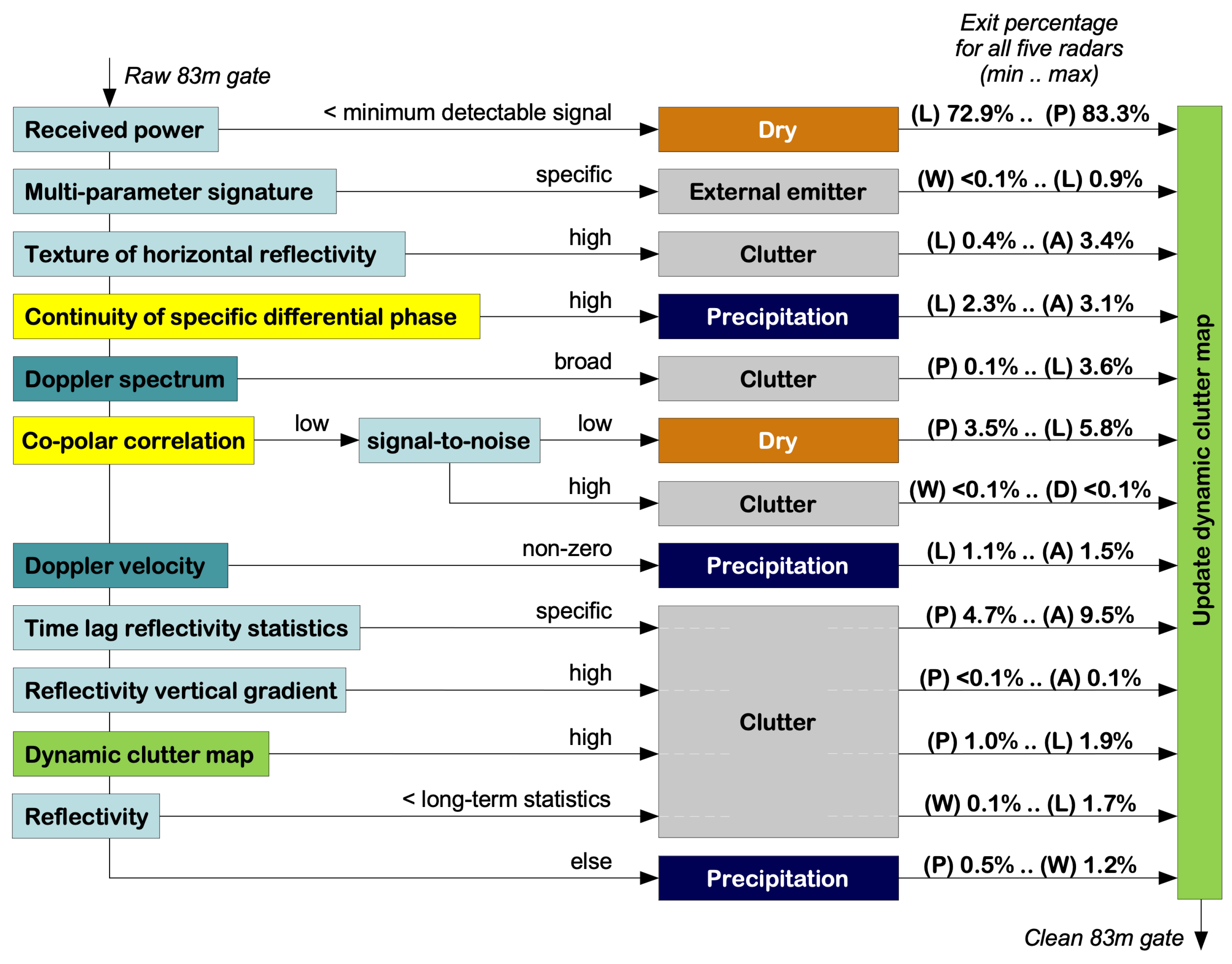
4.10. Data Processing and Product Generation

As mentioned in Section 3, two aspects are related to data processing in a mountainous region that require special attention, that is, the cancellation of mountain returns (ground clutter) and the proper treatment of beam shielding, visibility and VPR issues. As a result, the quality of radar measurements varies, to a great extent, in space and time, an aspect that needs to be taken into account in the generation of products for the users.

If a clutter signal is superimposed onto the signals of hydrometeors, it is necessary to subtract the former from the latter to obtain a clutter-free sample of the weather. This may be done by applying advanced filter techniques to the frequency domain [148] or following recent developments, preferably to the time domain [149,150], and this is commonly restricted to those gates that had been identified as potentially being cluttered in a preceding step using any robust clutter identification technique. Returns from mountains are often strong, which limits the usefulness of this method in a mountainous region. An alternative approach is to limit the spatial extent of clutter by using short pulses and to recover the meteorological signal from nearby clutter-free signals, see [3] and Figure 15. A variety of solutions have been proposed for the identification and cancellation of clutter signals, see, for instance, the fuzzy logic approaches presented in [151,152], which make ample use of the dual-polarisation capability of the French network. A multiparameter decision tree is applied in Switzerland on individual 83-m gates, see Figure 15 and Figure 18. The decision tree algorithm is built on the experience of the third radar generation [3,153,154] and has been refined with the deployment of the fourth generation of radars [1]. The approach makes use of polarimetric information (see the tests marked in yellow in Figure 18) but the decision tree was designed so that it would also work with single-polarisation. Cluttered gates will reliably be cancelled by the nonpolarimetric tests, should the polarimetric moments suffer from hardware instabilities, even though the number of erroneously cancelled weather signals will be somewhat higher. The order of the tests plays a crucial role and offers extra control over the performance of clutter cancellation, as each step involves taking a binary decision in a predefined sequence, which is an important difference between this and a fuzzy logic approach. There are many parameters in the decision tree, the settings of which are based on physical and statistical reasoning and careful fine-tuning over the years.

A large amount of literature is available on the correction of partial shielding and VPR effects, see [2,3,116,123,155,156] and references therein. Here, we limit the presentation to performance statistics routinely generated for real-time QPE products over Switzerland for hourly rainfall accumulations in the summer season. Table 3 shows the performance of two operational real-time QPE products, that is, a product based only on radar data (PRECIP) [4] and a product that combines PRECIP with rain gauge measurements using a space-time cokriging with external drift technique (CPC) [90]. The year 2011 has been excluded from these statistics, because of the installation of the first two radars of the fourth-generation network. The numbers in Table 3 show that a substantial improvement has been achieved over the years, which can be attributed to the deployment of two additional radars within the inner-Alpine regions in 2014 and 2016, improvements in the data quality control procedures and a number of innovations in the operational QPE algorithms. The rapidly growing data archives open the way towards new solutions that incorporate machine learning techniques, as demonstrated in Figure 19, which compares PRECIP and CPC with the results of RainForest, a new radar QPE algorithm currently being tested. RainForest was designed for use over complex orography and it makes use of dual-polarisation measurements and a machine learning approach [108]. The version of the RainForest algorithm that was used to calculate the data of Figure 19 has been optimised, simultaneously, for several different scores, including bias and scatter. If the aim is to optimise only one parameter, for instance scatter, RainForest can achieve even better scores. This demonstrates the great potential of machine learning approaches for customised applications optimised for specific needs.

It should be pointed out that any attempt to verify a QPE product using rain gauge measurements underrates the accuracy of radar products. First, rain gauge measurements are subject to errors, especially in a mountainous region, where the instrument is exposed to wind and a considerable part of precipitation falls as snow. Second, there is a substantial difference in the catching surface of a rain gauge and the spatial resolution of a radar pixel (representativeness error), see, for instance, [157]. Therefore, the differences between the QPE and the reference rain gauge are partly due to instrumental errors of the gauge and representativeness errors. This is less of a problem when the aim is to compare different methods (Figure 19) or different versions of algorithms (Table 3) in relative terms. However, caution is required when interpreting verification scores in absolute terms, for instance in the context of hydrological applications.

Table 3. Accuracy of real-time radar precipitation estimates for two operational products, a radar-only QPE (PRECIP) [4] versus a radar rain gauge merging with a cokriging with external drift technique (CPC) [90]. Accuracy is expressed as scatter in dB, see Figure 19, for hourly precipitation amounts in the summer months JJA. The scatter has decreased over the years, which points to a continuous improvement of the QPE algorithms. Automatic rain gauges of the whole of Switzerland are used for the evaluation. The tested rain gauge was left out of the cokriging (cross-validation) for the radar rain gauge combined QPE. The shown numbers are based on standardised procedures that are routinely used for verification purposes; no manual data selection or tuning was performed.

	1997	2005	2007	2009	2012	2014	2016	2018	2020
		2006	2008	2010	2013	2015	2017	2019	2021
Number of radars	3	3	3	3	3	3/4	5	5	5
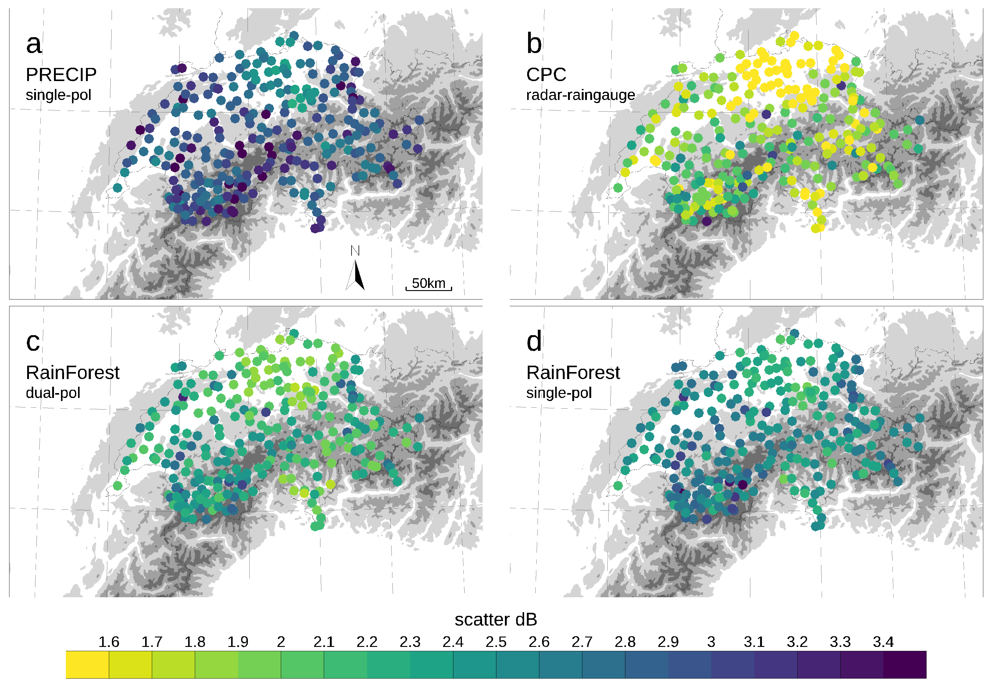
Scatter in dB, hourly precipitation, the whole of Switzerland
Radar-only	4.0	2.9	2.9	2.9	2.9	2.9	2.7	2.8	2.5
Radar rain gauge		2.5	2.3	2.4	2.2	2.1	1.9	1.9	1.7

Several other radar products, that have not been described in detail here, such as echo tops, vertically integrated liquid water (VIL) and wind speed, direction and shear estimated in the presence of radar echoes from precipitation, insects and Bragg scatter, are also available, see, for instance, [112] for an overview. As for QPE, the data processing has to be adapted to the particular situation over complex orography.

4.11. Multisource Data Integration

One way of coping with the limitations of radar measurements over complex orography is to combine them with data from other sources, such as rain gauge measurements, satellite imagery, lightning data, ground observations of hail and NWP output.

An obvious approach, which has a long history, is the merging of radar QPE with rainfall measurements from rain gauges, see, for instance, the evaluation of different techniques presented in [158], the method proposed in [159] and references therein. This approach can also be used, in principle, in mountainous regions. However, the merging of radar and rain gauge data can only deliver good results if both data streams have passed a rigorous automatic data quality control, which is a particularly demanding task for complex orography. A space-time cokriging with external drift technique, specifically developed for operational real-time radar rain gauge merging in mountainous Switzerland (CPC), was presented in [90] and was mentioned in the previous section. The CPC algorithm published in 2014 [90] has been extended to 5-min disaggregation [92] and many aspects have been refined with a particular focus on robustness and a proper treatment of the gradients in convective cells.

In addition to measurements from radar and rain gauges, it is also possible to add snow measurements conducted on glaciers [125,160,161], or fields of precipitation retrieved from satellite data, see, for instance, [162,163] for two studies over the European Alps.

In the cases mentioned before, independent estimates of the same variable, that is, the precipitation rate at the ground, were combined in one value. The combination of radar, satellite, lightning and NWP data in multisource thunderstorm tracking and nowcasting systems represent a different case. These various sources provide different but complementary information. When combined, they form a comprehensive picture of thunderstorms and the related hazards. For examples of thunderstorm nowcasting systems, developed for the use in complex orography, see [93,94,107,164].

A third type of real-time multisource data integration is the seamless blending [59,85,88] of radar QPE, Lagrangian radar extrapolation nowcasts [87,165] and NWP forecasts, following the pioneering work of [166,167]. These blending methods all involve radar nowcasts being seamlessly blended with NWP forecasts, while taking into account the respective skills of the two sources as a function of the lead time. The blended product starts from the radar QPE at time zero. Over the first few hours, it gives large weights to the Lagrangian radar extrapolation nowcast, and then seamlessly blends with the NWP forecasts for longer lead times. The blending also works in a probabilistic manner. Figure 3 shows the skill of a probabilistic Lagrangian radar extrapolation nowcast, an NWP ensemble forecast and a Bayesian blending of the two, averaged over four precipitation events in the central European Alps. The blending can also take place in multiple stages of the processing, as is the case of [59], where NWP forecasts of growth and decay over the orography were used to locally modify precipitation rates inside a Lagrangian radar extrapolation.

Hail is another example for which multisource data integration can be used. Single-polarisation techniques, used to estimate the probability and maximum expected size of hail, combine three-dimensional radar reflectivity measurements with information on the height of the zero-degree isotherm, which is commonly taken from NWP models. These single-polarisation radar hail products have routinely been used for hail monitoring in mountainous regions for many years, see, for instance, [52,54]. Dual-polarisation offers the possibility of identifying hail and other types of hydrometeors [99], as well as the level of mixing of different hydrometeor types [100], in the pulse volume of a radar measurement. Since 2015, hail has also been monitored in Switzerland by means of a crowdsourcing approach, based on a reporting function in the popular MeteoSwiss weather app. In the hail season of 2021 alone, the app users submitted 100,000 reports of hail observed on the ground in real time, an impressive number compared to the small size of the country, that is, 41,000 km

^{2}

. In addition, a network of 80 automatic hail sensors has been deployed in the three hail hot spots, that is, in central Switzerland, southern Ticino and over the Jura mountains. A drone, equipped with a high-resolution camera, has been used to take pictures of hail stones on green areas, such as football fields, shortly after a hailstorm, as a fourth option to obtain information on hail. Research on combining the different sources of hail information is ongoing; for the first results, see [75,98].

4.12. Modelling and Propagation of Uncertainty and End-to-End Processing Chains

Various approaches have been presented in the literature to assess the space-time error structure of radar measurements. Most of them refer to the uncertainty in radar QPE. Two fundamentally different approaches can be used to assess QPE uncertainties. In the first approach, the radar QPE is compared with a reference, typically measurements from rain gauges; see, for instance, [168]. In the second approach, the uncertainty is estimated using a model. The methods presented in [124,169], for instance, can be used to model the uncertainty that results from VPR and space-time variations of the drop size distribution, respectively. Not only is the amplitude of the uncertainties needed for most applications, but also its correlation in space and time, that is, the full covariance matrix of radar errors. The amplitude and the space-time correlation in a mountainous region exhibit a distinct dependence on the location, which needs to be taken into account, see [170].

The uncertainties in radar QPE are large, especially for a mountainous region with severe beam shielding and VPR issues. It has often been stated that the uncertainties in rainfall measurements need to be below 10% for hydrological applications, a requirement that is difficult to satisfy with a long-range surveillance radar sited on a mountain top (or with rain gauges). It is therefore tempting to reject the use of radar QPE for hydrological modelling and for the issuing of warnings of heavy precipitation, flash floods and debris flows. From the authors’ experience this is not a wise decision. First, some of the stochastic uncertainties are averaged when the rainfall is integrated in the hydrological processes in space and time, depending on the catchment and application. Second, other uncertainties of similar magnitude are involved in the hydrological system and the decision process. The decision makers are used to dealing with uncertainties. It is practically impossible to predict a debris flow. However, a simple statistical model, based on real-time radar data, and trained on a number of past events, will likely provide useful information to those decision makers who are managing the risks in a catchment prone to debris flows. In fact, thunderstorm, flash flood and debris flow warnings automatically generated from radar measurements have turned out to be of high practical value, in spite of the large uncertainties, as shown for the various applications in the Swiss Alps listed in Section 2.2.

Ensemble approaches play a central role in the modelling of radar errors and in studies of uncertainty propagation in hydrometeorological forecasting, see [171] for a review. There have been two major related European initiatives, the COST-731 action, the aim of which was to investigate the propagation of uncertainties in end-to-end hydrometeorological forecast systems [67], and MAP D-PHASE, a WMO forecast demonstration project that was held in the European Alps [70]. COST-731 and D-PHASE brought meteorologists, hydrologists and end users together and were ideal test beds to quantify the role of uncertainties in the context of real applications. The two initiatives triggered a number of unique experiments that coupled ensembles of radar QPE, Lagrangian nowcasts and NWP forecasts with hydrological models [66,68,109,170] and fostered the quantitative use of radar measurements in complex orography, despite the often large uncertainties.

4.13. Specific Needs and Customised Applications

In Section 2.2, we briefly presented a number of customised radar nowcasting systems that have been developed and configured to respond to the specific needs of users. However, there is yet another example of a recently developed application that is worth mentioning, related to hail and the specific needs of the building industry and insurance sector.

Both the northern and southern sides of the European Alps are areas with a comparatively high frequency of hail [52,53]. Two radar products are routinely generated in Switzerland to describe hail, POH and MESHS. In addition, there is the polarimetric hydrometeor classification, which has two hail classes (Figure 7). POH indicates the probability of hail, MESHS instead indicates the maximum expected diameter of hail stones from severe hail. The two products have been available for 20 years and were used to build the data base of a recently established set of climatological maps of hail in Switzerland (www.hagelklima.ch, accessed on 14 December 2021). POH and MESHS both refer to a reference area of one square kilometre. However, in the building industry and the insurance sector, the area of interest often corresponds to the size of a single building.

It is important to know the size of the largest hail stone that hits a building. The reference area is thus much smaller than a square kilometre, that is, around 100 m

^{2}

for a detached house or 250 m

^{2}

for an office complex. A transformation had to be found to estimate the largest hail size on a smaller reference area of the order of 100 or 250 square metres, starting from the MESHS climatology. Strictly speaking, this is not possible, unless we know the exact size distribution of hail and how the hail stones are distributed within the square kilometre of interest. For hail protection guidelines, it is possible to make assumptions on the average shape of the size distributions and the average spatial distribution within the square kilometre. These assumptions are then used to derive an arithmetic rule to transform an MESHS value, representing 1 km

^{2}

, into the size of the largest expected hail stone over a smaller area of the order of a building. Figure 20 presents such a transformation, LEHA, which was derived from hail size distributions observed in Switzerland during Grossversuch IV [172] and tested for plausibility with measurements from the recently deployed network of automatic hail sensors. LEHA involves a strong simplification, considering how complex the distribution of hailstone sizes is in reality. It is intended to give a rough estimate of hail diameters in areas of the size of a building for hail protection purposes.

5. Concluding Remarks

In complex orography scientists, engineers, technicians and the users of weather radars are faced with several major problems. The solutions developed for flat regions do not work, if not adapted to the particular situation, and the sources of errors are manifold. In this paper, it has been shown how the problems can be addressed in an operational context. The presented solutions and practical applications demonstrate the large potential and practical value of weather radars in a mountainous region, in spite of the harsh conditions and limitations.

Diversity has turned out to be beneficial, for several aspects. With a combination of different types of radar sites (“plain”, “offside”, “peak” and “valley”), one has a better chance of properly sampling precipitating clouds over the foreland, the foothills, the upslope region and in the inner parts of a major mountain range. It is crucial to combine different sources of information in parallel for hardware acceptance testing, monitoring and calibration. For QPE, a weighted combination of all the measurements in the vertical column above a ground pixel, which come from different elevation angles and radars, results in more accurate estimates of ground-level precipitation rates than single-sweep and single-radar approaches. It is recommended, for hydrological applications and the issuing of automatic heavy rainfall warnings, to combine, in parallel, in the sense of an ensemble, different types of QPE products (single polarisation, dual polarisation, radar rain gauge merging). For automatic hail reports at an airport, it is recommended to combine single-polarisation hail products, such as POH and MESHS, dual-polarisation hydrometeor classification and, ideally, also ground measurements of hail.

Machine learning approaches have great potential to complement algorithms based on physics, as demonstrated by many recent publications, see, for instance, [58,107,108,173]. The use of artificial intelligence has been accelerated by the continuously increasing computer power, easy access to libraries with advanced algorithms, rapidly growing archives of high quality data, and the ever-increasing demands of the users. An area with great potential for development is that of customised machine learning solutions designed and trained for specific applications. However, these data-centric approaches come with some drawbacks, which need to be addressed in future research. Other innovation paths concern the integration of crowdsourcing data, a first step of which was shown in [98], distributed adaptive sensing [141] and new radar technologies, such as phased-array antennas. It remains to be seen how these can successfully be used in complex orography.

Author Contributions

Conceptualization, writing—original draft preparation, U.G.; writing—review and editing, methodology, investigation, M.B., L.C., M.G., U.G., A.H., M.S. and I.V.S.; supervision, B.C. All authors have read and agreed to the published version of the manuscript.

Funding

This work was funded by the Federal Office of Meteorology and Climatology MeteoSwiss. The research on the usage of dual-polarisation measurements was cofunded by and done in close collaboration with the Alexis Berne group at EPFL. The research by Daniele Nerini and Loris Foresti was funded by SNF, under Ambizione grant PZ00P2_161316. The network of 80 automatic hail sensors was funded by Mobiliar and deployed by inNET Monitoring AG. Research on hail was cofunded by Mobiliar and conducted in close collaboration with the Olivia Martius group at University of Bern.

Acknowledgments

The authors are grateful to Peter Binder for his constant encouragement and support provided during and after the renewal of the radar network. The first author is indebted for the training in radar meteorology he received from Jürg Joss, Albert Waldvogel and Isztar Zawadzki. Thanks go to Philipp Schmid for providing Figure 9, to Rudi Kaltenböck for Figure 2, and to Daniel Wolfensberger for the data in Figure 19 and Figure 20. Thanks also go to Daniele Nerini, who provided Figure 3 and Figure 4, which are part of his PhD thesis done in collaboration with Loris Foresti (MeteoSwiss) and Heini Wernli (ETH). The comments and suggestions of two anonymous reviewers were greatly appreciated.

Conflicts of Interest

The authors declare no conflict of interest.

Abbreviations

The following abbreviations are used in this manuscript:

anaprop	Anomalous propagation
COSMO	The NWP model of the Consortium for Small-scale Modeling
CPC	Product identifier for radar rain gauge QPE
JJA	June, July and August
K $_{D P}$	Specific differential phase, a dual-polarisation parameter
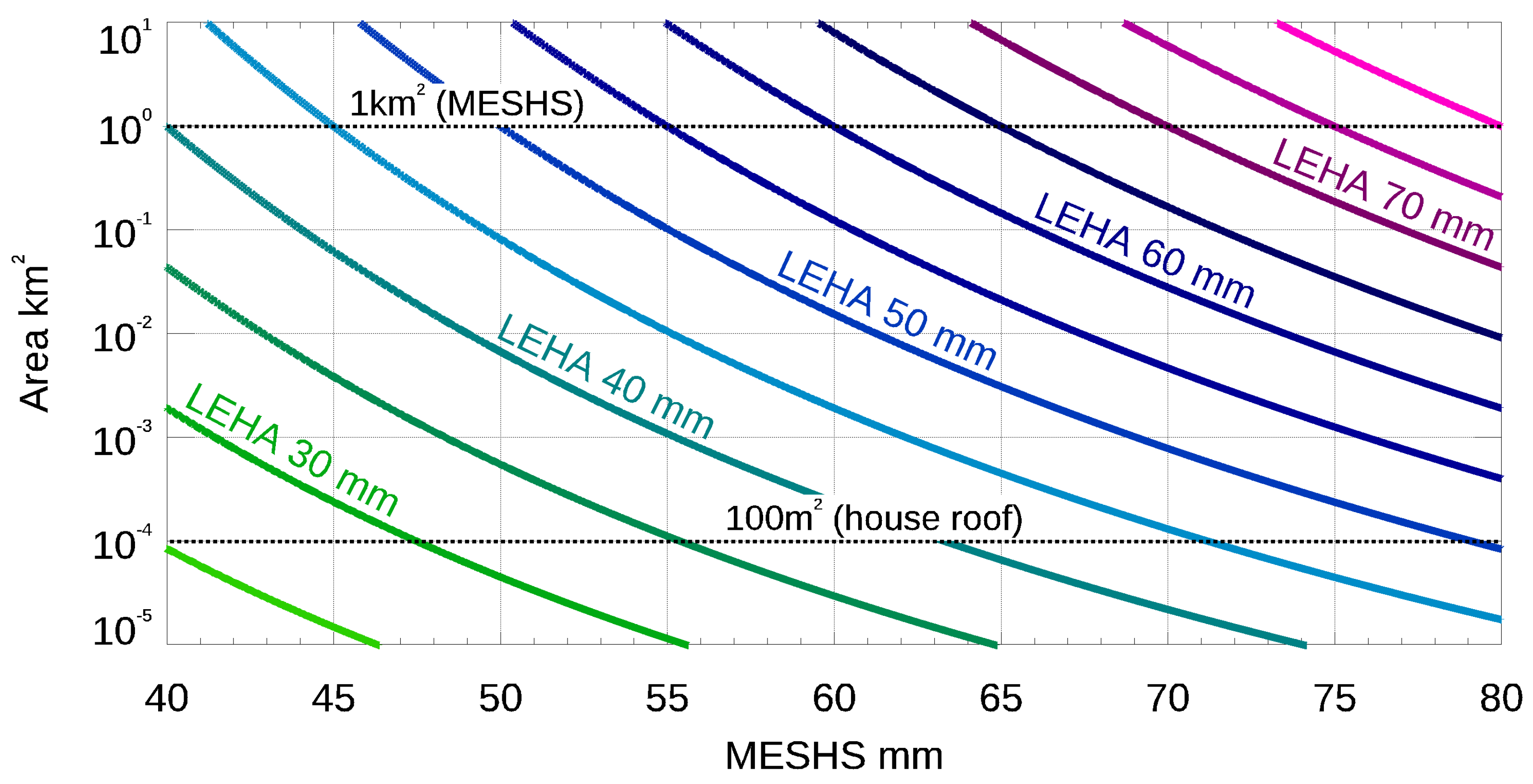
LEHA	Largest expected hail size on a reference area
MDS	Minimum detectable signal
METAR	Meteorological terminal air report
NWP	Numerical weather prediction
MESHS	Maximum expected severe hail size
POH	Probability of hail
PRF	Pulse repetition frequency
QPE	Quantitative precipitation estimation
RLAN	Radio local area network
ROEL	Receiver mounted over elevation
Rx	Receiver
SYNOP	Surface synoptic observation
TR-limiter	Transmit-receive limiter (a device used to protect a receiver from a transmit signal)
TRT	Thunderstorm radar tracking
VIL	Vertically integrated liquid water
Z $_{D R}$	Differential reflectivity, a dual-polarisation parameter

References

Germann, U.; Boscacci, M.; Gabella, M.; Schneebeli, M. Weather radar in Switzerland. In From Weather Observations to Atmospheric and Climate Sciences in Switzerland; Willemse, S., Furger, M., Eds.; VDF: Zurich, Switzerland, 2016. [Google Scholar] [CrossRef]
Joss, J.; Waldvogel, A. Precipitation measurement and hydrology. In Radar in Meteorology: Battan Memorial and 40th Anniversary Radar Meteorology Conference; Atlas, D., Ed.; Amer. Meteor. Soc.: Boston, US, USA, 1990; pp. 577–597. [Google Scholar] [CrossRef]
Joss, J.; Lee, R.L. The Application of RadarGauge Comparisons to Operational Precipitation Profile Corrections. J. Appl. Meteorol. 1995, 34, 2612–2630. [Google Scholar] [CrossRef] [Green Version]
Germann, U.; Galli, G.; Boscacci, M.; Bolliger, M. Radar precipitation measurement in a mountainous region. Q. J. R. Meteorol. Soc. 2006, 132, 1669–1692. [Google Scholar] [CrossRef]
Germann, U.; Boscacci, M.; Gabella, M.; Sartori, M. Peak performance—Radar design for the prediction in the Swiss Alps. Meteorol. Technol. Int. 2015, 4, 42–45. [Google Scholar]
Germann, U.; i Ventura, J.F.; Gabella, M.; Hering, A.; Sideris, I.; Calpini, B. Alpine weather radar: Triggering innovation. Meteorol. Technol. Int. 2016, 4, 62–65. [Google Scholar]
Germann, U.; Nerini, D.; Sideris, I.; Foresti, L.; Hering, A.; Calpini, B. Real-time radar—A new Alpine radar network. Meteorol. Technol. Int. 2017, 4, 88–92. [Google Scholar]
Kaltenboeck, R. New generation of dual polarized weather radars in Austria. In Proceedings of the Seventh European Conference on Radar in Meteorology and Hydrology, Toulouse, France, 24–29 June 2012; p. 6. [Google Scholar]
Beck, J.; Bousquet, O. Using Gap-Filling Radars in Mountainous Regions to Complement a National Radar Network: Improvements in Multiple-Doppler Wind Syntheses. J. Appl. Meteor. Climatol. 2013, 52, 1836–1850. [Google Scholar] [CrossRef] [Green Version]
i Ventura, J.F.; Tabary, P. The New French Operational Polarimetric Radar Rainfall Rate Product. J. Appl. Meteor. Climatol. 2013, 52, 1817–1835. [Google Scholar] [CrossRef]
Yu, N.; Gaussiat, N.; Tabary, P. Polarimetric X-band weather radars for quantitative precipitation estimation in mountainous regions. Q. J. R. Meteorol. Soc. 2018, 144, 2603–2619. [Google Scholar] [CrossRef]
Delrieu, G.; Caoudal, S.; Creutin, J.D. Feasibility of Using Mountain Return for the Correction of Ground-Based X-Band Weather Radar Data. J. Atmos. Oceanic Technol. 1997, 14, 368–385. [Google Scholar] [CrossRef]
Delrieu, G.; Serrar, S.; Guardo, E.; Creutin, J.D. Rain Measurement in Hilly Terrain with X-Band Weather Radar Systems: Accuracy of Path-Integrated Attenuation Estimates Derived from Mountain Returns. J. Atmos. Oceanic Technol. 1999, 16, 405–416. [Google Scholar] [CrossRef]
Delrieu, G.; Khanal, A.K.; Yu, N.; Cazenave, F.; Boudevillain, B.; Gaussiat, N. Preliminary investigation of the relationship between differential phase shift and path-integrated attenuation at the X band frequency in an Alpine environment. Atmos. Meas. Tech. 2020, 13, 3731–3749. [Google Scholar] [CrossRef]
Bechini, R.; Cremonini, R. The weather radar system of north-western Italy: An advanced tool for meteorological surveillance. In Proceedings of the Second European Conference on Radar in Meteorology and Hydrology, Delft, The Netherlands, 18–22 November 2002; Copernicus: Gottingen, Germany, 2002; pp. 400–404. [Google Scholar]
Gabella, M.; Joss, J.; Perona, G. Optimizing quantitative precipitation estimates using a non-coherent and a coherent radar operating on the same area. J. Geophys. Res. 2000, 105, 2237–2245. [Google Scholar] [CrossRef]
Dinku, T.; Anagnostou, E.N.; Borga, M. Improving Radar-Based Estimation of Rainfall over Complex Terrain. J. Appl. Meteor. 2002, 41, 1163–1178. [Google Scholar] [CrossRef]
Fornasiero, A.; Bech, J.; Alberoni, P.P. Enhanced radar precipitation estimates using a combined clutter and beam blockage correction technique. Nat. Hazards Earth Syst. Sci. 2006, 6, 697–710. [Google Scholar] [CrossRef] [Green Version]
Minciardi, R.; SAcile, R.; Siccardi, F. Optimal Planning of a Weather Radar Network. J. Atmos. Oceanic Technol. 2003, 20, 1251–1263. [Google Scholar] [CrossRef]
Cremonini, R.; Bechini, R. Heavy Rainfall Monitoring by Polarimetric C-Band Weather Radars. Water 2010, 2, 838–848. [Google Scholar] [CrossRef]
Vulpiani, G.; Montopoli, M.; Passeri, L.D.; Gioia, A.G.; Giordano, P.; Marzano, F.S. On the Use of Dual-Polarized C-Band Radar for Operational Rainfall Retrieval in Mountainous Areas. J. Appl. Meteorol. Climatol. 2012, 51, 405–425. [Google Scholar] [CrossRef]
Montopoli, M.; Roberto, N.; Adirosi, E.; Gorgucci, E.; Baldini, L. Investigation ofWeather Radar Quantitative Precipitation Estimation Methodologies in Complex Orography. Atmosphere 2017, 8, 34. [Google Scholar] [CrossRef] [Green Version]
Crum, T.D.; Alberty, R.L. The WSR-88D and the WSR-88D Operational Support Facility. Bull. Amer. Meteor. Soc. 1993, 74, 1669–1688. [Google Scholar] [CrossRef]
Klazura, G.E.; Imy, D.A. A Description of the Initial Set of Analysis Products Available from the NEXRAD WSR-88D System. Bull. Amer. Meteor. Soc. 1993, 74, 1293–1312. [Google Scholar] [CrossRef] [Green Version]
Zhang, G.; Mahale, V.N.; Putnam, B.J.; Qi, Y.; Cao, Q.; Byrd, A.D.; Bukovcic, P.; Zrnic, D.S.; Gao, J.; Xue, M.; et al. Current Status and Future Challenges of Weather Radar Polarimetry: Bridging the Gap between Radar Meteorology/Hydrology/Engineering and Numerical Weather Prediction. Adv. Atmos. Sci. 2019, 76, 571–588. [Google Scholar] [CrossRef] [Green Version]
Westrick, K.J.; Mass, C.F.; Colle, B.A. The Limitations of the WSR-88D Radar Network for Quantitative Precipitation Measurement over the Coastal Western United States. Bull. Amer. Meteor. Soc. 1999, 80, 2289–2298. [Google Scholar] [CrossRef]
Maddox, R.A.; Zhang, J.; Gourley, J.J.; Howard, K.W. Weather Radar Coverage over the Contiguous United States. Wea. Forecast. 2002, 17, 927–934. [Google Scholar] [CrossRef]
Zhang, J.; Qi, Y.; Kingsmill, D.; Howard, K. Radar-Based Quantitative Precipitation Estimation for the Cool Season in Complex Terrain: Case Studies from the NOAA Hydrometeorology Testbed. J. Hydrometeor. 2012, 13, 1836–1854. [Google Scholar] [CrossRef]
Chen, H.; Cifelli, R.; Chandrasekar, V.; Ma, Y.Z. A Flexible Bayesian Approach to Bias Correction of Radar-Derived Precipitation Estimates over Complex Terrain: Model Design and Initial Verification. J. Hydrometeor. 2019, 20, 2367–2382. [Google Scholar] [CrossRef]
Chen, H.; Cifelli, R.; White, A.B. Improving Operational Radar Rainfall Estimates Using Profiler Observations Over Complex Terrain in Northern California. IEEE Trans. Geosci. Remote Sens. 2020, 58, 1821–1832. [Google Scholar] [CrossRef]
Kwon, S.; Jung, S.H.; Lee, G. Inter-comparison of radar rainfall rate using Constant Altitude Plan Position Indicator and hybrid surface rainfall maps. J. Hydrol. 2015, 531, 234–247. [Google Scholar] [CrossRef]
Chang, P.L.; Lin, P.F.; Jou, B.J.D.; Zhang, J. An Application of Reflectivity Climatology in Constructing Radar Hybrid Scans over Complex Terrain. J. Atmos. Oceanic Technol. 2009, 26, 1315–1327. [Google Scholar] [CrossRef]
Ye, B.Y.; Lee, G.; Park, H.M. Identification and removal of non-meteorological echoes in dual-polarization radar data based on a fuzzy logic algorithm. Adv. Atmos. Sci. 2015, 32, 1217–1230. [Google Scholar] [CrossRef]
Yu, C.K.; Cheng, L.W. Radar Observations of Intense Orographic Precipitation Associated with Typhoon Xangsane (2000). Mon. Wea. Rev. 2008, 136, 497–521. [Google Scholar] [CrossRef] [Green Version]
Liou, Y.C.; Chang, S.F.; Sun, J. An Application of the Immersed Boundary Method for Recovering the Three-Dimensional Wind Fields over Complex Terrain Using Multiple-Doppler Radar Data. Mon. Wea. Rev. 2012, 140, 1603–1619. [Google Scholar] [CrossRef] [Green Version]
Tsai, C.L.; Kim, K.; Liou, Y.C.; Lee, G.; Yu, C.K. Impacts of Topography on Airflow and Precipitation in the Pyeongchang Area Seen from Multiple-Doppler Radar Observations. Mon. Wea. Rev. 2018, 146, 3401–3424. [Google Scholar] [CrossRef]
Min, C.; Chen, S.; Gourley, J.J.; Chen, H.; Zhang, A.; Huang, Y.; Huang, C. Coverage of China New Generation Weather Radar Network. Adv. Meteorol. 2019, 2019, 5789358. [Google Scholar] [CrossRef]
Shi, Z.; Wei, F.; Chandrasekar, V. Radar-based quantitative precipitation estimation for the identification of debris flow occurrence over earthquake-affected regions in Sichuan, China. Nat. Hazards Earth Syst. Sci. 2018, 18, 765–780. [Google Scholar] [CrossRef] [Green Version]
Gou, Y.; Ma, Y.; Chen, H.; Wen, Y. Radar-derived quantitative precipitation estimation in complex terrain over the eastern Tibetan Plateau. Atmos. Res. 2018, 203, 286–297. [Google Scholar] [CrossRef]
Gou, Y.; Ma, Y.; Chen, H.; Yin, J. Utilization of a C-band Polarimetric Radar for Severe Rainfall Event Analysis in Complex Terrain over Eastern China. Remote Sens. 2019, 11, 22. [Google Scholar] [CrossRef] [Green Version]
Gray, W.R.; Seed, A.W. The characterisation of orographic rainfall. Meteor. Appl. 2000, 7, 105–119. [Google Scholar] [CrossRef]
Talchabhadel, R.; Ghimire, G.R.; Sharma, S.; Dahal, P.; Panthi, J.; Baniya, R.; Pudashine, J.; Thapa, B.R.; Shakti, P.; Parajuli, B. Weather radar in Nepal: Opportunities and challenges in a mountainous region. Weather, 2021; early view. [Google Scholar] [CrossRef]
Bendix, J.; Fries, A.; Zárate, J.; Trachte, K.; Rollenbeck, R.; Pucha-Cofrep, F.; Paladines, R.; Palacios, I.; Orellana, J.; Oñate-Valdivieso, F.; et al. RadarNet-Sur First Weather Radar Network in Tropical High Mountains. Bull. Amer. Meteor. Soc. 2017, 98, 1235–1254. [Google Scholar] [CrossRef]
Rotunno, R.; Ferretti, R. Mechanisms of Intense Alpine Rainfall. J. Atmos. Sci. 2001, 58, 1732–1749. [Google Scholar] [CrossRef]
Rotunno, R.; Houze, R.A. Lessons on orographic precipitation from the Mesoscale Alpine Programme. Q. J. R. Meteorol. Soc. 2007, 133, 811–830. [Google Scholar] [CrossRef]
Houze, R.A., Jr. Orographic effects on precipitating clouds. Rev. Geophys. 2012, 50, 47. [Google Scholar] [CrossRef]
Germann, U.; Joss, J. Variograms of Radar Reflectivity to Describe the Spatial Continuity of Alpine Precipitation. J. Appl. Meteor. 2001, 40, 1042–1059. [Google Scholar] [CrossRef]
Houze, R.A., Jr.; James, C.N.; Medina, S. Radar observations of precipitation and airflow on the Mediterranean side of the Alps: Autumn 1998 and 1999. Q. J. R. Meteorol. Soc. 2001, 127, 2537–2558. [Google Scholar] [CrossRef]
Medina, S.; Houze, R.A., Jr. Air motions and precipitation growth in alpine storms. Q. J. R. Meteorol. Soc. 2003, 129, 345–371. [Google Scholar] [CrossRef] [Green Version]
Panziera, L.; Germann, U. The relation between airflow and orographic precipitation on the southern side of the Alps as revealed by weather radar. Q. J. R. Meteorol. Soc. 2010, 136, 222–238. [Google Scholar] [CrossRef]
Panziera, L.; James, C.N.; Germann, U. Mesoscale organization and structure of orographic precipitation producing flash floods in the Lago Maggiore region. Q. J. R. Meteorol. Soc. 2015, 141, 224–248. [Google Scholar] [CrossRef]
Nisi, L.; Martius, O.; Hering, A.; Kunz, M.; Germann, U. Spatial and temporal distribution of hailstorms in the Alpine region: A long-term, high resolution, radar-based analysis. Q. J. R. Meteorol. Soc. 2016, 142, 1590–1604. [Google Scholar] [CrossRef]
Nisi, L.; Hering, A.; Germann, U.; Martius, O. A 15-year hail streak climatology for the Alpine region. Q. J. R. Meteorol. Soc. 2018, 144, 1429–1449. [Google Scholar] [CrossRef] [Green Version]
Foresti, L.; Sideris, I.V.; Panziera, L.; Nerini, D.; Germann, U. A 10-year radar-based analysis of orographic precipitation growth and decay patterns over the Swiss Alpine region. Q. J. R. Meteorol. Soc. 2018, 144, 2277–2301. [Google Scholar] [CrossRef]
Panziera, L.; Gabella, M.; Germann, U.; Martius, O. A 12-year radar-based climatology of daily and sub-daily extreme precipitation over the Swiss Alps. Int. J. Climatol. 2018, 38, 3749–3769. [Google Scholar] [CrossRef]
Panziera, L.; Germann, U.; Gabella, M.; Mandapaka, P.V. NORA–Nowcasting of Orographic Rainfall by means of Analogues. Q. J. R. Meteorol. Soc. 2011, 137, 2106–2123. [Google Scholar] [CrossRef]
Foresti, L.; Panziera, L.; Mandapaka, P.V.; Germann, U.; Seed, A. Retrieval of analogue radar images for ensemble nowcasting of orographic rainfall. Meteor. Appl. 2015, 22, 141–155. [Google Scholar] [CrossRef]
Foresti, L.; Sideris, I.V.; Nerini, D.; Beusch, L.; Germann, U. Using a 10-Year Radar Archive for Nowcasting Precipitation Growth and Decay: A Probabilistic Machine Learning Approach. Wea. Forecast. 2019, 34, 1547–1569. [Google Scholar] [CrossRef]
Sideris, I.V.; Foresti, L.; Nerini, D.; Germann, U. NowPrecip: Localized precipitation nowcasting in the complex terrain of Switzerland. Q. J. R. Meteorol. Soc. 2020, 146, 1768–1800. [Google Scholar] [CrossRef]
Council, N.R. Flash Flood Forecasting over Complex Terrain: With an Assessment of the Sulphur Mountain NEXRAD in Southern California; The National Academies Press: Washington DC, USA, 2005; p. 206. [Google Scholar] [CrossRef]
Westrelin, S.; Meriaux, P.; Tabary, P.; Aubert, Y. Hydrometeorological risks in Mediterranean mountainous areas— RHYTMME Project: Risk Management based on a Radar Network. In Proceedings of the Seventh European Conference on Radar in Meteorology and Hydrology, Toulouse, France, 24–29 June 2012; p. 6. [Google Scholar]
Panziera, L.; Gabella, M.; Zanini, S.; Hering, A.; Germann, U.; Berne, A. A radar-based regional extreme rainfall analysis to derive the thresholds for a novel automatic alert system in Switzerland. Hydrol. Earth Syst. Sci. 2016, 20, 2317–2332. [Google Scholar] [CrossRef] [Green Version]
Leuenberger, D.; Rossa, A. Revisiting the latent heat nudging scheme for the rainfall assimilation of a simulated convective storm. Meteor. Atmos. Phys. 2004, 98, 195–215. [Google Scholar] [CrossRef]
Borga, M.; Anagnostou, E.N.; Frank, E. On the use of real-time radar rainfall estimates for flood prediction in mountainous basins. J. Geophys. Res. Atmos. 2000, 105, 2269–2280. [Google Scholar] [CrossRef]
Berenguer, M.; Corral, C.; Sánchez-Diezma, R.; Sempere-Torres, D. Hydrological Validation of a Radar-Based Nowcasting Technique. J. Hydrometeor. 2005, 6, 532–549. [Google Scholar] [CrossRef] [Green Version]
Zappa, M.; Jaun, S.; Germann, U.; Walser, A.; Fundel, F. Superposition of three sources of uncertainties in operational flood forecasting chains. Atmos. Res. 2011, 100, 246–262. [Google Scholar] [CrossRef]
Rossa, A.; Liechti, K.; Zappa, M.; Bruen, M.; Germann, U.; Haase, G.; Keil, C.; Krahe, P. The COST 731 Action: A review on uncertainty propagation in advanced hydro-meteorological forecast systems. Atmos. Res. 2011, 100, 150–167. [Google Scholar] [CrossRef]
Liechti, K.; Zappa, M.; Fundel, F.; Germann, U. Probabilistic evaluation of ensemble discharge nowcasts in two nested Alpine basins prone to flash floods. Hydrol. Process. 2013, 27, 5–17. [Google Scholar] [CrossRef]
Binder, P. MAP—Mesoscale Alpine Programme Design Proposal. NOAA Tech. Rep. ERL402-NHELM2, MeteoSwiss, 1996. Available online: http://iacweb.ethz.ch/doc/publications/1996_BinderSchar_MAP_DP.pdf (accessed on 14 December 2021).
Rotach, M.W.; Ambrosetti, P.; Appenzeller, F.A.C.; Arpagaus, M.; Behrendt, H.B.A.; Bouttier, F.; Buzzi, A.; Corazza, M.; Davolio, S.; Denhard, M.; et al. MAP D-PHASE: Real-Time Demonstration of Weather Forecast Quality in the Alpine Region. Bull. Amer. Meteor. Soc. 2009, 90, 1321–1336. [Google Scholar] [CrossRef] [Green Version]
Savina, M. The Use of a Cost-Effective X-Band Weather Radar in Alpine Region. Ph.D. Thesis, ETH Zurich, Zurich, Germany, 2011. [Google Scholar] [CrossRef]
Wulfmeyer, V.; Behrendt, A.; Kottmeier, C.; Corsmeier, U.; Barthlott, C.; Craig, G.C.; Hagen, M.; Althausen, D.; Aoshima, F.; Arpagaus, M.; et al. The Convective and Orographically-induced Precipitation Study (COPS): The scientific strategy, the field phase, and research highlights. Q. J. R. Meteorol. Soc. 2011, 137, 3–30. [Google Scholar] [CrossRef]
Mandapaka, P.V.; Germann, U.; Panziera, L. Diurnal cycle of precipitation over complex Alpine orography: Inferences from high-resolution radar observations. Q. J. R. Meteorol. Soc. 2013, 139, 1025–1046. [Google Scholar] [CrossRef]
Mott, R.; Scipión, D.; Schneebeli, M.; Dawes, N.; Berne, A.; Lehning, M. Orographic effects on snow deposition patterns in mountainous terrain. J. Geophys. Res. Atmos. 2014, 119, 1419–1439. [Google Scholar] [CrossRef] [Green Version]
Trefalt, S.; Martynov, A.; Barras, H.; Besic, N.; Hering, A.M.; Lenggenhager, S.; Noti, P.; Rötlisberger, M.; Schemm, S.; Germann, U.; et al. A severe hail storm in complex topography in Switzerland— Observations and processes. Atmos. Res. 2018, 209, 78–94. [Google Scholar] [CrossRef] [Green Version]
i Ventura, J.F.; Pineda, N.; Besic, N.; Grazioli, J.; Hering, A.; Van Der Velde, O.A.; Romero, D.; Sunjerga, A.; Mostajabi, A.; Azadifar, M.; et al. Analysis of the lightning production of convective cells. Atmos. Meas. Tech. 2019, 12, 5573–5591. [Google Scholar] [CrossRef] [Green Version]
Boettcher, M.; Schäfler, A.; Sprenger, M.; Sodemann, H.; Kaufmann, S.; Voigt, C.; Schlager, H.; Summa, D.; Di Girolamo, P.; Nerini, D.; et al. Lagrangian matches between observations from aircraft, lidar and radar in a warm conveyor belt crossing orography. Atmos. Chem. Phys. 2021, 21, 5477–5498. [Google Scholar] [CrossRef]
Martius, O.; Hering, A.; Kunz, M.; Manzato, A.; Mohr, S.; Nisi, L.; Trefalt, S. Challenges and Recent Advances in Hail Research. Bull. Am. Meteorol. Soc. 2018, 99, ES51–ES54. [Google Scholar] [CrossRef] [Green Version]
Barton, Y.; Sideris, I.V.; Raupach, T.H.; Gabella, M.; Germann, U.; Martius, O. A multi-year assessment of sub-hourly gridded precipitation for Switzerland based on a blended radar—Rain-gauge dataset. Int. J. Climatol. 2020, 40, 5208–5222. [Google Scholar] [CrossRef]
Nisi, L.; Hering, A.; Germann, U.; Schroeer, K.; Barras, H.; Kunz, M.; Martius, O. Hailstorms in the Alpine region: Diurnal cycle, 4D-characteristics, and the nowcasting potential of lightning properties. Q. J. R. Meteorol. Soc. 2020, 146, 4170–4194. [Google Scholar] [CrossRef]
Fluck, E.; Kunz, M.; Geissbuehler, P.; Ritz, S.P. Radar-based assessment of hail frequency in Europe. Nat. Hazards Earth Syst. Sci. 2021, 21, 683–701. [Google Scholar] [CrossRef]
Germann, U.; Zanini, S. Condizioni meteorologiche estreme. In L’alluvione del ’78: Testimonianze e Riflessioni; Museo di valmaggia, Ed.; Armando Dadò Editore: Locarno, Switzerland, 2020; pp. 57–68. [Google Scholar]
Gabella, M.; Mantovani, R. The floods of 13–16 October 2000 in Piedmont (Italy): Quantitative precipitation estimates using radar and a network of gauges. Weather 2001, 56, 337–351. [Google Scholar] [CrossRef]
Marra, F.; Nikolopoulos, E.I.; Creutin, J.D.; Borga, M. Radar rainfall estimation for the identification of debris-flow occurrence thresholds. J. Hydrol. 2014, 519, 1607–1619. [Google Scholar] [CrossRef]
Nerini, D.; Foresti, L.; Leuenberger, D.; Robert, S.; Germann, U. A Reduced-Space Ensemble Kalman Filter Approach for Flow-Dependent Integration of Radar Extrapolation Nowcasts and NWP Precipitation Ensembles. Mon. Wea. Rev. 2019, 147, 987–1006. [Google Scholar] [CrossRef]
Nerini, D. Ensemble Precipitation Nowcasting: Limits to Prediction, Localization and Seamless Blending. Ph.D. Thesis, ETH Zurich, Zurich, Germany, 2019. [Google Scholar] [CrossRef]
Mandapaka, P.V.; Germann, U.; Panziera, L.; Hering, A. Can Lagrangian Extrapolation of Radar Fields Be Used for Precipitation Nowcasting over Complex Alpine Orography? Wea. Forecast. 2012, 27, 28–49. [Google Scholar] [CrossRef]
Pulkkinen, S.; Nerini, D.; Pérez Hortal, A.A.; Velasco-Forero, C.; Seed, A.; Germann, U.; Foresti, L. Pysteps: An open-source Python library for probabilistic precipitation nowcasting (v1.0). Geosci. Model Dev. 2019, 12, 4185–4219. [Google Scholar] [CrossRef] [Green Version]
Gabella, M.; Joss, J.; Perona, G.; Galli, G. Accuracy of rainfall estimates by two radars in the same Alpine environment using gauge adjustment. J. Geophys. Res. 2001, 106, 5139–5150. [Google Scholar] [CrossRef] [Green Version]
Sideris, I.V.; Gabella, M.; Erdin, R.; Germann, U. Real-time radar–rain-gauge merging using spatio-temporal co-kriging with external drift in the alpine terrain of Switzerland. Q. J. R. Meteorol. Soc. 2014, 140, 1097–1111. [Google Scholar] [CrossRef]
Gabella, M.; Panziera, L.; Sideris, I.; Boscacci, M.; Wolfensberger, D.; Clementi, L.; Germann, U. Twelve years of operational real-time hourly precipitation estimation in the Alps: Better performance of the radar-only and radar-gauge products in recent years. In Proceedings of the 11th International Workshop on Precipitation in Urban Areas, Pontresina, Switzerland, 5–7 December 2018; p. 5. [Google Scholar]
Barton, Y.; Sideris, I.V.; Germann, U.; Martius, O. A method for real-time temporal disaggregation of blended radar-rain gauge precipitation fields. Meteor. Appl. 2020, 27, 14. [Google Scholar] [CrossRef] [Green Version]
Hering, A.M.; Morel, C.; Galli, G.; Sénési, S.; Ambrosetti, P.; Boscacci, M. Nowcasting thunderstorms in the Alpine region using a radar based adaptive thresholding scheme. In Proceedings of the 3th European Conference on Radar in Meteorology and Hydrology, Gotland, Sweden, 6–10 September 2004; Copernicus: Gottingen, Germany, 2004; pp. 206–211. [Google Scholar]
Hering, A.M.; Germann, U.; Boscacci, M.; Sénési, S. Operational nowcasting of thunderstorms in the Alps during MAP D-PHASE. In Proceedings of the 5th European Conference on Radar in Meteorology and Hydrology, Helsinki, Finland, 30 June–4 July 2008; Copernicus: Gottingen, Germany, 2008; p. 5. [Google Scholar]
Hering, A.M.; Nisi, L.; Bruna, G.D.; Gaia, M.; Nerini, D.; Ambrosetti, P.; Hamann, U.; Trefalt, S.; Germann, U. Fully automated thunderstorm warnings and operational nowcasting at MeteoSwiss. In Proceedings of the European Conference on Severe Storms, Wiener Neustadt, Austria, 14–18 September 2015; p. 3. [Google Scholar]
Grazioli, J.; Leuenberger, A.; Peyraud, L.; i Ventura, J.F.; Gabella, M.; Hering, A.; Germann, U. Adaptive thunderstorm measurements using C-band and X-band radar data. IEEE Geosci. Remote Sens. Lett. 2019, 16, 1673–1677. [Google Scholar] [CrossRef]
Hirschi, E.; Hering, A.; Germann, U. Damage limitation—A short-term hail warning system. Meteorological Technology International, 15 November 2019; pp. 66–69. [Google Scholar]
Barras, H.; Hering, A.; Martynov, A.; Noti, P.A.; Germann, U.; Martius, O. Experiences with >50,000 Crowdsourced Hail Reports in Switzerland. Bull. Amer. Meteor. Soc. 2019, 100, 1429–1440. [Google Scholar] [CrossRef]
Besic, N.; i Ventura, J.F.; Grazioli, J.; Gabella, M.; Germann, U.; Berne, A. Hydrometeor classification through statistical clustering of polarimetric radar measurements: A semi-supervised approach. Atmos. Meas. Tech. 2016, 9, 4425–4445. [Google Scholar] [CrossRef] [Green Version]
Besic, N.; Gehring, J.; Praz, C.; i Ventura, J.F.; Grazioli, J.; Gabella, M.; Germann, U.; Berne, A. Unraveling hydrometeor mixtures in polarimetric radar measurements. Atmos. Meas. Tech. 2018, 11, 4847–4866. [Google Scholar] [CrossRef] [Green Version]
Germann, U. Vertical wind profile by Doppler radars. In Mesoscale Alpine Programme (MAP) Newsletters; MeteoSwiss: Locarno-Monti, Switzerland, 1999. [Google Scholar]
Tabary, P.; Scialom, G.; Germann, U. Real-Time Retrieval of the Wind from Aliased Velocities Measured by Doppler Radars. J. Atmos. Oceanic Technol. 2001, 18, 875–882. [Google Scholar] [CrossRef]
Feldmann, M.; James, C.N.; Boscacci, M.; Leuenberger, D.; Gabella, M.; Germann, U.; Wolfensberger, D.; Berne, A. R2D2: A Region-Based Recursive Doppler Dealiasing Algorithm for Operational Weather Radar. J. Atmos. Ocean. Technol. 2020, 37, 2341–2356. [Google Scholar] [CrossRef]
Feldmann, M.; Germann, U.; Gabella, M.; Berne, A. A Characterisation of Alpine Mesocyclone Occurrence. Weather. Clim. Dyn. Discuss. 2021, 2, 1225–1244. [Google Scholar] [CrossRef]
Leuenberger, D. High-Resolution Radar Rainfall Assimilation: Exploratory Studies with Latent Heat Nudging. Ph.D. Thesis, ETH Zurich, Zurich, Germany, 2005. [Google Scholar] [CrossRef]
i Ventura, J.F.; Lainer, M.; Schauwecker, Z.; Grazioli, J.; Germann, U. Pyrad: A Real-Time Weather Radar Data Processing Framework Based on Py-ART. J. Open Res. Softw. 2020, 8, 28. [Google Scholar] [CrossRef]
Leinonen, J.; Hamann, U.; Germann, U.; Mecikalski, J.R. Nowcasting thunderstorm hazards using machine learning: The impact of data sources on performance. Nat. Hazards Earth Syst. Sci. Discuss. 2021, 2021, 1–28. [Google Scholar] [CrossRef]
Wolfensberger, D.; Gabella, M.; Boscacci, M.; Germann, U.; Berne, A. RainForest: A random forest algorithm for quantitative precipitation estimation over Switzerland. Atmos. Meas. Tech. 2021, 14, 3169–3193. [Google Scholar] [CrossRef]
Liechti, K.; Fundel, F.; Germann, U.; Zappa, M. Flood nowcasting in the Southern Swiss Alps using radar ensemble. IAHS Publ. 2012, 351, 496–501. [Google Scholar]
Gabella, M.; Leuenberger, A. Dual-Polarization Observations of Slowly Varying Solar Emissions from a Mobile X-Band Radar. Sensors 2017, 17, 1185. [Google Scholar] [CrossRef] [Green Version]
Gabella, M.; Boscacci, M.; Sartori, M.; Germann, U. Calibration Accuracy of the Dual-Polarization Receivers of the C-Band Swiss Weather Radar Network. Atmosphere 2016, 7, 76. [Google Scholar] [CrossRef] [Green Version]
World Meteorological Organization. Guide to Instruments and Methods of Observations: Volume III— Observing Systems. Technical Report WMO-No. 8, World Meteorological Organization, 7 bis, avenue de la Paix, CH-1211 Geneva 2, Switzerland. 2018. Available online: https://library.wmo.int (accessed on 14 December 2021).
Delrieu, G.; Creutin, J.D.; Andrieu, H. Simulation of Radar Mountain Returns Using a Digitized Terrain Model. J. Atmos. Oceanic Technol. 1995, 12, 1038–1049. [Google Scholar] [CrossRef] [Green Version]
Gabella, M.; Perona, G. Simulation of the Orographic Influence on Weather Radar Using a Geometric-Optics Approach. J. Atmos. Oceanic Technol. 1998, 15, 1485–1494. [Google Scholar] [CrossRef]
Friedrich, K.; Germann, U.; Tabary, P. Influence of Ground Clutter Contamination on Polarimetric Radar Parameters. J. Atmos. Oceanic Technol. 2009, 26, 251–269. [Google Scholar] [CrossRef] [Green Version]
Pellarin, T.; Delrieu, G.; Saulnier, G.M.; Andrieu, H.; Vignal, B.; Creutin, J.D. Hydrologic Visibility of Weather Radar Systems Operating in Mountainous Regions: Case Study for the Ardèche Catchment (France). J. Hydrometeor. 2002, 3, 539–555. [Google Scholar] [CrossRef]
Bech, J.; Gjertsen, U.; Haase, G. Modelling weather radar beam propagation and topographical blockage at northern high latitudes. Q. J. R. Meteorol. Soc. 2007, 133, 1191–1204. [Google Scholar] [CrossRef]
Ryzhkov, A.V.; Zrnic, D.S. Radar Polymetry for Weather Observations; Springer: Berlin/Heidelberg, Germany, 2019. [Google Scholar] [CrossRef]
Zrnic, D.S.; Ryzhkov, A.V. Advantages of rain measurements using specific differential phase. J. Atmos. Oceanic Technol. 1996, 13, 454–464. [Google Scholar] [CrossRef] [Green Version]
Vivekanandan, J.; Yates, D.N.; Brandes, E.A. The Influence of Terrain on Rainfall Estimates from Radar Reflectivity and Specific Propagation Phase Observations. J. Atmos. Oceanic Technol. 1999, 16, 837–845. [Google Scholar] [CrossRef]
Friedrich, K.; Germann, U.; Gourley, J.J.; Tabary, P. Effects of Radar Beam Shielding on Rainfall Estimation for the Polarimetric C-Band Radar. J. Atmos. Oceanic Technol. 2007, 24, 1839–1859. [Google Scholar] [CrossRef] [Green Version]
Thompson, R.; Illingworth, A.; Ovens, J. Emission: A simple new technique to correct rainfall estimates from attenuation due to both radome and heavy rainfall. Weather. Radar Hydrol. 2012, 351, 39–44. [Google Scholar]
Germann, U.; Joss, J. Mesobeta Profiles to Extrapolate Radar Precipitation Measurements above the Alp. J. Appl. Meteor. 2002, 41, 542–557. [Google Scholar] [CrossRef]
Lee, G.W.; Zawadzki, I. Variability of Drop Size Distributions: Time-Scale Dependence of the Variability and Its Effects on Rain Estimation. J. Appl. Meteor. 2005, 44, 241–255. [Google Scholar] [CrossRef]
Gugerli, R.; Gabella, M.; Huss, M.; Salzmann, N. Can Weather Radars Be Used to Estimate Snow Accumulation on Alpine Glaciers? An Evaluation Based on Glaciological Surveys. J. Hydrometeor. 2020, 21, 2943–2962. [Google Scholar] [CrossRef]
Capozzi, V.; Montopoli, M.; Bracci, A.; Adirosi, E.; Baldini, L.; Vulpiani, G.; Budillon, G. Retrieval of snow precipitation rate from polarimetric X-band radar measurements in Southern Italy Apennine mountains. Atmos. Res. 2020, 236, 104796. [Google Scholar] [CrossRef]
Germann, U. Radome attenuation—A serious limiting factor for quantitative radar measurements? Meteor. Z. 1999, 8, 85–90. [Google Scholar] [CrossRef]
Kurri, M.; Huuskonen, A. Measurements of the Transmission Loss of a Radome at Different Rain Intensities. J. Atmos. Oceanic Technol. 2008, 25, 1590–1599. [Google Scholar] [CrossRef]
Frasier, S.J.; Kabeche, F.; Ventura, J.F.; Al-Sakka, H.; Tabary, P.; Beck, J.; Bousquet, O. In-Place Estimation of Wet Radome Attenuation at X Band. J. Atmos. Oceanic Technol. 2013, 30, 917–928. [Google Scholar] [CrossRef]
Kucera, P.A.; Krajewski, W.F.; Young, C.B. Radar Beam Occultation Studies Using GIS and DEM Technology: An Example Study of Guam. J. Atmos. Oceanic Technol. 2004, 21, 995–1006. [Google Scholar] [CrossRef] [Green Version]
Khanal, A.K.; Delrieu, G.; Cazenave, F.; Boudevillain, B. Radar Remote Sensing of Precipitation in High Mountains: Detection and Characterization of Melting Layer in the Grenoble Valley, French Alps. Atmosphere 2019, 10, 784. [Google Scholar] [CrossRef] [Green Version]
den Heuvel, F.V.; Gabella, M.; Germann, U.; Berne, A. Characterisation of the melting layer variability in an Alpine valley based on polarimetric X-band radar scans. Atmos. Meas. Tech. 2018, 11, 5181–5198. [Google Scholar] [CrossRef] [Green Version]
Gabella, M.; Sartori, M.; Progin, O.; Germann, U. Acceptance tests and monitoring of the next generation polarimetric weather radar network in Switzerland. In Proceedings of the 2013 International Conference on Electromagnetics in Advanced Applications (ICEAA), Turin, Italy, 9–13 September 2013. [Google Scholar]
Saltikoff, E.; Kurri, M.; Leijnse, H.; Barbosa, S.; Stiansen, K. Maintenance Keeps Radars Running. Bull. Amer. Meteor. Soc. 2017, 98, 1833–1840. [Google Scholar] [CrossRef]
Scipión, D.E.; Mott, R.; Lehning, M.; Schneebeli, M.; Berne, A. Seasonal small-scale spatial variability in alpine snowfall and snow accumulation. Wat. Resour. Res. 2013, 49, 1446–1457. [Google Scholar] [CrossRef] [Green Version]
Allegretti, M.; Bertoldo, S.; Prato, A.; Lucianaz, C.; Rorato, O.; Notarpietro, R.; Gabella, M. X-Band Mini Radar for Observing and Monitoring Rainfall Events. Atmos. Clim. Sci. 2012, 2, 290–297. [Google Scholar] [CrossRef]
Vollbracht, D.; Sartori, M.; Gabella, M. Absolute dual-polarization radar calibration: Temperature dependence and stability with focus on antenna-mounted receivers and Noise Source-generated reference signal. In Proceedings of the 8th European Conference on Radar in Meteorology and Hydrology, Garmisch-Partenkirchen, Germany, 1–5 September 2014; pp. 111–122. [Google Scholar]
Vollbracht, D.; Ridene, D.; Gekat, F. Receiver over Elevation (ROEL) Weather Radar System Design and its Advantages. In Proceedings of the 12th URSI Commission F Triennial Open Symposium on Wave Propagation and Remote Sensing, Garmisch-Partenkirchen, Germany, 8–11 March 2011. [Google Scholar]
Vaccarono, M.; Bechini, R.; Chandrasekar, C.V.; Cremonini, R.; Cassardo, C. An integrated approach to monitoring the calibration stability of operational dual-polarization radars. Atmos. Meas. Tech. 2016, 9, 5367–5383. [Google Scholar] [CrossRef] [Green Version]
Frech, M.; Hubbert, J. Monitoring the differential reflectivity and receiver calibration of the German polarimetric weather radar network. Atmos. Meas. Tech. 2020, 13, 1051–1069. [Google Scholar] [CrossRef] [Green Version]
Wang, Y.; Chandrasekar, V. Quantitative Precipitation Estimation in the CASA X-band Dual-Polarization Radar Network. J. Atmos. Oceanic Technol. 2010, 27, 1665–1676. [Google Scholar] [CrossRef]
Hollemann, I.; Huuskonen, A.; Kurri, M.; Beekhuis, H. Operational Monitoring of Weather Radar Receiving Chain Using the Sun. J. Atmos. Oceanic Technol. 2010, 27, 159–166. [Google Scholar] [CrossRef]
Holleman, I.; Huuskonen, A.; Gill, R.; Tabary, P. Operational Monitoring of Radar Differential Reflectivity Using the Sun. J. Atmos. Oceanic Technol. 2010, 27, 881–887. [Google Scholar] [CrossRef]
Gabella, M.; Sartori, M.; Boscacci, M.; Germann, U. Vertical and horizontal polarization observations of slowly varying solar emissions from operational Swiss weather radars. Atmosphere 2015, 6, 50–59. [Google Scholar] [CrossRef] [Green Version]
Gabella, M. On the Spectral and Polarimetric Signatures of a Bright Scatterer before and after Hardware Replacement. Remote Sens. 2021, 13, 919. [Google Scholar] [CrossRef]
i Ventura, J.F.; Boumahmoud, A.A.; Fradon, B.; Dupuy, P.; Tabary, P. Long-term monitoring of French polarimetric radar data quality and evaluation of several polarimetric quantitative precipitation estimators in ideal conditions for operational implementation at C-band. Q. J. R. Meteorol. Soc. 2012, 138, 2212–2228. [Google Scholar] [CrossRef]
i Ventura, J.F.; Boscacci, M.; Clementi, L.; Sideris, I.V.; Gabella, M.; Germann, U. Rad4Alp, The new Swiss Doppler Polarimetric Weather Radar Network: Data Quality and First Results. In Proceedings of the 36th Conference on Radar Meteorology, Breckenridge, CO, USA, 16–20 September 2013; p. 5. [Google Scholar]
Siggia, A.D.; Passarelli, R.E. Gaussian model adaptive processing (GMAP) for improved ground clutter cancellation and moment calculation. In Proceedings of the Third European Conference on Radar in Meteorology and Hydrology ERAD, Visby, Sweden, 6–10 September 2004; 2004; pp. 67–73. [Google Scholar]
Nguyen, C.M.; Chandrasekar, V. Gaussian Model Adaptive Processing in Time Domain (GMAP-TD) for Weather Radars. J. Atmos. Oceanic Technol. 2013, 30, 2571–2584. [Google Scholar] [CrossRef]
Hubbert, J.C.; Meymaris, G.; Romatschke, U.; Dixon, M. Using a Regression Ground Clutter Filter to Improve Weather Radar Signal Statistics: Theory and Simulations. J. Atmos. Oceanic Technol. 2021, 38, 1353–1375. [Google Scholar] [CrossRef]
Gourley, J.J.; Tabary, P.; du Chatelet, J.P. A Fuzzy Logic Algorithm for the Separation of Precipitating from Nonprecipitating Echoes Using Polarimetric Radar Observations. J. Atmos. Oceanic Technol. 2007, 24, 1439–1451. [Google Scholar] [CrossRef]
Berenguer, M.; Sempere-Torres, D.; Corral, C.; Sánchez-Diezma, R. A Fuzzy Logic Technique for Identifying Nonprecipitating Echoes in Radar Scans. J. Atmos. Oceanic Technol. 2006, 23, 1157–1180. [Google Scholar] [CrossRef] [Green Version]
Germann, U. Spatial Continuity of Precipitation, Profiles of Radar Reflectivity and Precipitation Measurements in the Alps. Ph.D. Thesis, ETH Zurich, Zurich, Germany, 2000. [Google Scholar] [CrossRef]
Germann, U.; Joss, J. Operational measurement of precipitation in mountainous terrain. In Weather Radar: Principles and Advanced Applications; Meischner, P., Ed.; Springer: Berlin/Heidelberg, Germany, 2004; pp. 52–77. [Google Scholar]
Vignal, B.; Galli, G.; Joss, J.; Germann, U. Three Methods to Determine Profiles of Reflectivity from Volumetric Radar Data to Correct Precipitation Estimates. J. Appl. Meteor. 2000, 39, 1715–1726. [Google Scholar] [CrossRef]
Franco, M.; Sánchez-Diezma, R.; Sempere-Torres, D. Improvements in weather radar rain rate estimates using a method for identifying the vertical profile of reflectivity from volume radar scans. Meteor. Z. 2006, 15, 521–536. [Google Scholar] [CrossRef]
Villarini, G.; Mandapaka, P.V.; Krajewski, W.F.; Moore, R.J. Rainfall and sampling uncertainties: A rain gauge perspective. J. Geophys. Res. Atmos. 2008, 113, 12. [Google Scholar] [CrossRef]
Goudenhoofdt, E.; Delobbe, L. Evaluation of radar-gauge merging methods for quantitative precipitation estimates. Hydrol. Earth Syst. Sci. 2009, 13, 195–203. [Google Scholar] [CrossRef] [Green Version]
Tabary, P.; Boumahmoud, A.A.; Andrieu, H.; Thompson, R.J.; Illingworth, A.J.; Bouar, E.L.; Testud, J. Evaluation of two “integrated” polarimetric Quantitative Precipitation Estimation (QPE) algorithms at C-band. J. Hydrol. 2011, 405, 248–260. [Google Scholar] [CrossRef]
Gugerli, R.; Guidicelli, M.; Gabella, M.; Huss, M.; Salzmann, N. Multi-sensor analysis of monthly gridded snow precipitation on alpine glaciers. Adv. Sci. Res. 2021, 18, 7–20. [Google Scholar] [CrossRef]
Guidicelli, M.; Gugerli, R.; Gabella, M.; Marty, C.; Salzmann, N. Continuous Spatio-Temporal High-Resolution Estimtaes of SWE Across the Swiss Alps—A Statistical Two-Step Approach for High-Mountain Topography. Front. Earth Sci. 2021, 9, 664648. [Google Scholar] [CrossRef]
Gabella, M.; Speirs, P.; Hamann, U.; Germann, U.; Berne, A. Measurement of Precipitation in the Alps Using Dual-Polarization C-Band Ground-Based Radars, the GPM Spaceborne Ku-Band Radar, and Rain Gauges. Remote Sens. 2017, 9, 1147. [Google Scholar] [CrossRef] [Green Version]
Speirs, P.; Gabella, M.; Berne, A. A Comparison between the GPM Dual-Frequency Precipitation Radar and Ground-Based Radar Precipitation Rate Estimates in the Swiss Alps and Plateau. J. Hydrometeor. 2017, 18, 1247–1269. [Google Scholar] [CrossRef]
Nisi, L.; Ambrosetti, P.; Clementi, L. Nowcasting severe convection in the Alpine region: The COALITION approach. Q. J. R. Meteorol. Soc. 2014, 140, 1684–1699. [Google Scholar] [CrossRef]
Germann, U.; Zawadzki, I. Scale-Dependence of the Predictability of Precipitation from Continental Radar Images. Part I: Description of the Methodology. Mon. Wea. Rev. 2002, 130, 2859–2873. [Google Scholar] [CrossRef]
Seed, A.W. A Dynamic and Spatial Scaling Approach to Advection Forecasting. J. Appl. Meteor. 2003, 42, 381–388. [Google Scholar] [CrossRef]
Bowler, N.E.; Pierce, C.E.; Seed, A.W. STEPS: A probabilistic precipitation forecasting scheme which merges an extrapolation nowcast with downscaled NWP. Q. J. R. Meteorol. Soc. 2006, 132, 2127–2155. [Google Scholar] [CrossRef]
Mandapaka, P.V.; Krajewski, W.F.; Ciach, G.J.; Villarini, G.; Smith, J.A. Estimation of radar-rainfall error spatial correlation. Ad. Water Resour. 2009, 32, 1020–1030. [Google Scholar] [CrossRef]
Bellon, A.; Lee, G.W.; Zawadzki, I. Error Statistics of VPR Corrections in Stratiform Precipitation. J. Appl. Meteor. 2005, 44, 998–1015. [Google Scholar] [CrossRef] [Green Version]
Germann, U.; Berenguer, M.; Sempere-Torres, D.; Zappa, M. REAL—Ensemble radar precipitation estimation for hydrology in a mountainous region. Q. J. R. Meteorol. Soc. 2009, 135, 445–456. [Google Scholar] [CrossRef] [Green Version]
Mandapaka, P.V.; Germann, U. Radar-Rainfall Error Models and Ensemble Generators. In Rainfall: State of Science; Testik, F., Gebremichael, M., Eds.; American Geophysical Union: Washington, DC, USA, 2010; pp. 247–264. [Google Scholar] [CrossRef] [Green Version]
Federer, B.; Waldvogel, A.; Schmid, W.; Schiesser, H.H.; Hampel, F.; Schweingruber, M.; Stahel, W.; Bader, J.; Mezeix, J.F.; Doras, N.; et al. Main results of Grossversuch IV. J. Appl. Meteor. Climatol. 1986, 25, 917–957. [Google Scholar] [CrossRef] [Green Version]
Ravuri, S.; Lenc, K.; Willson, M.; Kangin, D.; Lam, R.; Mirowski, P.; Fitzsimons, M.; Athanassiadou, M.; Kashem, S.; Madge, S.; et al. Skilful precipitation nowcasting using deep generative models of radar. Nature 2021, 597, 672–677. [Google Scholar] [CrossRef]

Figure 1. Map of the operational Swiss radar network which consists of 5 radars: La Dôle and Albis (since 1959, 1st generation), Monte Lema (since 1993, 3rd generation), Pointe de la Plaine Morte and Weissfluhgipfel (since 2014/2016, 4th generation). The heights of the radar sites and selected mountain peaks are in metres above sea level.

Figure 2. Re-routing and holding loops of air traffic during thunderstorms over the eastern Austrian Alps on 17 July 2010, 20:15. The aircraft trajectories correspond to a 10-min period. Only reflectivity values above 35 dBZ are shown; yellow corresponds to >40, red to >50 dBZ. Image courtesy of R. Kaltenböck.

Figure 3. The skill of ensemble forecasting in the nowcasting time frame of three different methods, that is, a stochastic Lagrangian extrapolation of radar fields [88], a state-of-the-art numerical weather prediction model in ensemble mode (COSMO-E), and a Bayesian blending of the previous two [85]. The analysis was conducted as a function of the spatial scale and for different rain rate thresholds by pooling data of four events for a total of 48 hours of precipitation. The fraction skill score, FSS, for precipitation >2 mm/h and a spatial scale of 32 km is shown here. This is the average of the four events shown in Figure 12 in [85], ©American Meteorological Society; used with permission.

Figure 4. The predictable scale of Lagrangian radar extrapolation nowcasts (solid lines) and COSMO-1 forecasts (dashed lines) as a function of the lead time. The COSMO-1 curves are shifted by 1.5 h to account for the computational requirements of numerical simulations. The computation time may be reduced in the future by increasing the update frequency of the NWP model. The evaluation spans data from the whole of 2018 and over a 640 km × 710 km domain centred over the European Alps. (a) The scale-aware normalised root-mean-square error, RMSE

_{n}

, for all analysed scales separately. Considering an RMSE

_{n}

of 1 as the limit of predictability, it is possible to identify the predictable scale for each lead time. This is shown in (b). Taken from [86].

Figure 4. The predictable scale of Lagrangian radar extrapolation nowcasts (solid lines) and COSMO-1 forecasts (dashed lines) as a function of the lead time. The COSMO-1 curves are shifted by 1.5 h to account for the computational requirements of numerical simulations. The computation time may be reduced in the future by increasing the update frequency of the NWP model. The evaluation spans data from the whole of 2018 and over a 640 km × 710 km domain centred over the European Alps. (a) The scale-aware normalised root-mean-square error, RMSE

_{n}

, for all analysed scales separately. Considering an RMSE

_{n}

of 1 as the limit of predictability, it is possible to identify the predictable scale for each lead time. This is shown in (b). Taken from [86].

Figure 5. (a) Automatic tracking, extrapolation and (b) severity ranking of thunderstorms [94]. All the thunderstorm cells (polygons) are shown in panel (a), whereas only cells above a certain severity are marked in panel (b). The number in the cells indicates the maximum cell vertically integrated liquid (VIL) water, which is one of the parameters used to compute cell severity. For this time step, there is one cell just slightly above the severity threshold (white ellipse, VIL 12 kg/m

^{2}

), one moderate cell (green), one severe cell (yellow) and one very severe cell (red, VIL 51 kg/m

^{2}

). The uncertainty of the cell position forecast is represented by the increasing size of the extrapolated ellipses. The underlying colour in (a) and (b) shows the precipitation rate (QPE). The data refer to 20 June 2021, 1400 UTC. The geographic domain corresponds to that of Figure 1.

Figure 5. (a) Automatic tracking, extrapolation and (b) severity ranking of thunderstorms [94]. All the thunderstorm cells (polygons) are shown in panel (a), whereas only cells above a certain severity are marked in panel (b). The number in the cells indicates the maximum cell vertically integrated liquid (VIL) water, which is one of the parameters used to compute cell severity. For this time step, there is one cell just slightly above the severity threshold (white ellipse, VIL 12 kg/m

^{2}

), one moderate cell (green), one severe cell (yellow) and one very severe cell (red, VIL 51 kg/m

^{2}

). The uncertainty of the cell position forecast is represented by the increasing size of the extrapolated ellipses. The underlying colour in (a) and (b) shows the precipitation rate (QPE). The data refer to 20 June 2021, 1400 UTC. The geographic domain corresponds to that of Figure 1.

Figure 6. Inauguration of a new railway bridge in the Grison Alps in eastern Switzerland in 2011. The new bridge is three metres higher than the old one and was built to protect the rails from increasing threats of flash floods and debris flows. A customised radar-based heavy precipitation warning system was put into operation on 7 August 2017. One day later, the nowcasting system issued its first warning, and a few minutes later the rails on the new bridge were flooded by a debris flow. Photograph courtesy of the Rhaetian Railway.

Figure 7. Hydrometeor types retrieved from polarimetric radar measurements in the original coordinate system of the polar volume scan [99]. The figure shows a vertical cross section through a hail cell on 27 May 2016. (a) The hail cell seen from the Albis radar at an azimuth angle of 57°. (b) View from the Weissfluhgipfel radar at an azimuth angle of 316°. The dashed vertical line indicates the intersection. For the positions of the two cross sections, see the thin dotted lines in Figure 1.

Figure 8. Nonmeteorological signals (clutter) in a Swiss radar composite map on a clear sky day with the clutter cancellation switched off. The data refer to 13 September 2021, at 05:15 UTC. The dashed rectangle corresponds to the domain shown in Figure 1. There are strong ground returns, >50 dBZ, in practically all the regions in Switzerland, which demonstrates the importance of rigorous and reliable clutter cancellation in the automatic warning context.

Figure 9. Registration of the noise level in the Albis radar receiver on 28 June 2021. The emissions from the wetted radome and the water in the atmosphere cause an increase in the noise level of more than 1.5 dB at the moment a severe hail cell approaching from the south-west passes over the radar. (a) Noise power as a function of time sampled at an elevation of 35° (red dots) and 40° (salmon dots). The measurement of a simple rain detector with three intensity classes installed on the tower of the radar is also indicated (blue). (b) The same noise power as in (a), here shown as a function of the azimuth, between 13:30 and 16:30 UTC, when the cell approaches the radar (salmon and red dots), and at 16:35 UTC (black), at the time the cell hits the radar. The grey ellipse indicates the mean and standard deviation of the wind at the radar site. The antenna occasionally points in the direction of the Sun and the Sun’s signal is superimposed onto the noise level (star), as automatically detected by the online Sun monitoring system. The exact value of the Sun’s signal depends on the relative position between the Sun and the centre of the beam, an aspect that is taken into account in the automatic monitoring of the receiver. All the red, salmon and black dots and stars are averages over 10° in the azimuth.

Figure 10. Cumulated fraction of the Swiss territory (x-axis) that is visible to the radar network below a certain height (y-axis). (a) Situation if data are available from 1 radar (Albis), 3 radars (Albis, Dôle and Lema) and all 5 radars (Albis, Dôle, Lema, Plaine Morte and Weissfluhgipfel). The areas in blue and green indicate the proportion of the atmosphere that is visible to the radar network, whereas the area in white corresponds to the proportion that is not visible, either due to shielding or clutter contamination. The calculations are based on echo and clutter statistics from 2020 referring to the three-dimensional volume above the 41,000 km

^{2}

Swiss territory. It should be noted that Albis is the lowest radar in Switzerland and is located on a hill near Zurich. The Dôle and Lema radars are located on mountain tops at intermediate heights (1.6 km above sea level), whereas the Plaine Morte and Weissfluhgipfel radars are situated on peaks close to 3 km above sea level in the inner part of the Alps, see also Figure 1. (b) Situation when the lowest radar, Albis, is missing, for instance, due to corrective maintenance. For QPE, the usefulness of measurements decreases with range because of the broadening of the beam. At a 115 km range, a one-degree beam has a width of 2 km. (c) The same as (a), but only using radar measurements up to a maximum range of 115 km.

Figure 10. Cumulated fraction of the Swiss territory (x-axis) that is visible to the radar network below a certain height (y-axis). (a) Situation if data are available from 1 radar (Albis), 3 radars (Albis, Dôle and Lema) and all 5 radars (Albis, Dôle, Lema, Plaine Morte and Weissfluhgipfel). The areas in blue and green indicate the proportion of the atmosphere that is visible to the radar network, whereas the area in white corresponds to the proportion that is not visible, either due to shielding or clutter contamination. The calculations are based on echo and clutter statistics from 2020 referring to the three-dimensional volume above the 41,000 km

^{2}

Swiss territory. It should be noted that Albis is the lowest radar in Switzerland and is located on a hill near Zurich. The Dôle and Lema radars are located on mountain tops at intermediate heights (1.6 km above sea level), whereas the Plaine Morte and Weissfluhgipfel radars are situated on peaks close to 3 km above sea level in the inner part of the Alps, see also Figure 1. (b) Situation when the lowest radar, Albis, is missing, for instance, due to corrective maintenance. For QPE, the usefulness of measurements decreases with range because of the broadening of the beam. At a 115 km range, a one-degree beam has a width of 2 km. (c) The same as (a), but only using radar measurements up to a maximum range of 115 km.

Figure 11. Four different types of radar sites used to monitor precipitating clouds over complex orography. The rays and the grey shading indicate the part of the atmosphere that can be seen by the “plain”, “peak” and “offside” radars. The range of visibility of the “valley” type is limited to the visible cone above that valley, which is not shown in the figure.

Figure 12. Precipitation along a vertical north–south cross section through the Alps, as seen by the five Swiss radars. Reflectivity measurements from each radar were converted into equivalent rainfall rates using a fixed Z–R relation and then accumulated over the whole of 2016. All five panels use the same colour scale. Ideally, all the radars would show the same picture, that is, have the same values for all the locations on the cross section. However, this is not the case, because of severe shielding, clutter cancellation and broadening of the beam with distance. The distance between the radar sites and the nearest point on the cross section is indicated after the name of each radar. For the position of the cross section, see the dashed line in Figure 1.

Figure 13. Picture of the radar on Pointe de la Plaine Morte, 2937 m above sea level. The lightning protection consists of two groups of lightning poles, one below the lowest point of the antenna, and the other one on top of the radome. This design results in minimal interference of the lightning poles on the radar beam and polarimetric measurements.

Figure 14. The Swiss volume scan consists of 20 elevation sweeps and is completed every 5 min. The antenna scans the atmosphere up to a maximum range of 246 km and maximum height of 18 km. The sequence follows an interleaved scheme with two half-volume scans (blue and yellow), which allows products to be generated every 2.5 min.

Figure 15. Reflectivity for horizontal polarisation in the Alps, where the main lobe of the beam of the Plaine Morte radar hits steep mountain crests; see also the mountains in the background of the photograph shown in Figure 13. The pulse length is 0.5 microseconds, which corresponds to 75 m. Reflectivity is sampled at a radial resolution of 83 m. (a) Reflectivity of ground clutter in a moment with clear sky conditions. (b) Reflectivity for a mixed situation with ground clutter superimposed onto precipitation signals. (c) The same time as (b), but for clean reflectivity data after clutter cancellation and radial integration for 500 m gates. The same colour scale is used for reflectivity as in Figure 8. (d) Differential phase shift, a key variable in the clutter cancellation algorithm (Section 4.10), for the same time as (b) and (c). The values range from 0 to

2 π

.

Figure 15. Reflectivity for horizontal polarisation in the Alps, where the main lobe of the beam of the Plaine Morte radar hits steep mountain crests; see also the mountains in the background of the photograph shown in Figure 13. The pulse length is 0.5 microseconds, which corresponds to 75 m. Reflectivity is sampled at a radial resolution of 83 m. (a) Reflectivity of ground clutter in a moment with clear sky conditions. (b) Reflectivity for a mixed situation with ground clutter superimposed onto precipitation signals. (c) The same time as (b), but for clean reflectivity data after clutter cancellation and radial integration for 500 m gates. The same colour scale is used for reflectivity as in Figure 8. (d) Differential phase shift, a key variable in the clutter cancellation algorithm (Section 4.10), for the same time as (b) and (c). The values range from 0 to

2 π

.

Figure 16. The antenna radiation pattern of the Plaine Morte radar, measured under real conditions, with the radome, at the site at 2937 m above sea level, after commissioning in 2014. The parabolic antenna has a diameter of 4.2 m and a gain of 45 dB. The measurements were made by an external receiver located on a nearby mountain.

Figure 17. Ageing TR-limiter on the Weissfluhgipfel radar, as revealed by the automatic noise source measurements in the horizontal (red) and vertical (green) polarisations (y-axis to the left), the difference between the two (blue), and samples of the Sun’s signal obtained online during normal operation (black dots, y-axis on the right).

Figure 18. In the Swiss radar network, clutter signals are cancelled at the radial resolution of 83-m gates, using a multiparameter decision tree, which combines single- (light blue), Doppler (dark blue) and dual-polarisation (yellow) information. The numbers at the exit of each test indicate the exit statistics for 2020. It shows the minimum and maximum values for the five radars, with the initial letter of the radar site in parenthesis. Considering all 5 radars, the algorithm has to make a decision for 51 million gates every 5 min, that is, 170,000 gates every second. It should be noted that a few strong clutter gates, erroneously classified as precipitation, may be enough to generate a false severe weather warning.

Figure 19. Performance of different QPE algorithms, evaluated at the automatic rain gauge locations, and expressed as the scatter in dB, a robust measure of the standard deviation [4,91]. The smaller the scatter is, the better the QPE algorithm. (a) PRECIP is a QPE product that is based on single-polarisation algorithms [4]. (b) CPC is based on geostatistical merging of PRECIP and rain gauge data [90]; to determine the scatter for CPC, the tested rain gauge was left out of the geostatistical merging (cross-validation). (c,d) RainForest is a recently developed QPE algorithm that uses machine learning and incorporates dual-polarisation data. For a detailed description and discussion of RainForest and the underlying data set, see [108]. (c) shows the performance of RainForest, including dual-polarisation data, whereas (d) shows RainForest trained and tested on only single-polarisation data. The geographic domain corresponds to that of Figure 1.

Figure 20. LEHA is an arithmetic rule that is used to transform an MESHS hail diameter (x-axis), referring to a 1 km

^{2}

pixel, to a smaller reference area (y-axis), which is typically the size of a building. The abbreviation LEHA stands for largest expected hail size on a reference area. For instance, a LEHA value of about 3.5 centimeters is obtained for an MESHS value of 5.5 cm and a house roof with a size of 100 m

^{2}

.

Figure 20. LEHA is an arithmetic rule that is used to transform an MESHS hail diameter (x-axis), referring to a 1 km

^{2}

pixel, to a smaller reference area (y-axis), which is typically the size of a building. The abbreviation LEHA stands for largest expected hail size on a reference area. For instance, a LEHA value of about 3.5 centimeters is obtained for an MESHS value of 5.5 cm and a house roof with a size of 100 m

^{2}

.

Publisher’s Note: MDPI stays neutral with regard to jurisdictional claims in published maps and institutional affiliations.

© 2022 by the authors. Licensee MDPI, Basel, Switzerland. This article is an open access article distributed under the terms and conditions of the Creative Commons Attribution (CC BY) license (https://creativecommons.org/licenses/by/4.0/).

Share and Cite

MDPI and ACS Style

Germann, U.; Boscacci, M.; Clementi, L.; Gabella, M.; Hering, A.; Sartori, M.; Sideris, I.V.; Calpini, B. Weather Radar in Complex Orography. Remote Sens. 2022, 14, 503. https://doi.org/10.3390/rs14030503

AMA Style

Germann U, Boscacci M, Clementi L, Gabella M, Hering A, Sartori M, Sideris IV, Calpini B. Weather Radar in Complex Orography. Remote Sensing. 2022; 14(3):503. https://doi.org/10.3390/rs14030503

Chicago/Turabian Style

Germann, Urs, Marco Boscacci, Lorenzo Clementi, Marco Gabella, Alessandro Hering, Maurizio Sartori, Ioannis V. Sideris, and Bertrand Calpini. 2022. "Weather Radar in Complex Orography" Remote Sensing 14, no. 3: 503. https://doi.org/10.3390/rs14030503

Note that from the first issue of 2016, this journal uses article numbers instead of page numbers. See further details here.

Article Menu

Weather Radar in Complex Orography

Abstract

1. Introduction

Outline

2. Practical Applications, Needs and Requirements

2.1. The Scales of Interest

2.2. Operational Applications in the Swiss Alps

2.3. Radar System Requirements

3. Challenges

3.1. Planning and Installation

3.2. Maintenance and Operation

3.3. Reflection and Shielding by the Terrain

3.4. Other Challenges

4. Solutions and Results

4.1. Design Considerations

4.2. Siting

4.3. Installation, Acceptance Testing and Lightning Protection

4.4. Radio Frequency and Polarimetry

4.5. Receiver over Elevation Design

4.6. Scanning the Atmosphere over Complex Orography

4.7. Pulse Length

4.8. Calibration, Monitoring and Control

4.9. Availability and Timeliness

4.10. Data Processing and Product Generation

4.11. Multisource Data Integration

4.12. Modelling and Propagation of Uncertainty and End-to-End Processing Chains

4.13. Specific Needs and Customised Applications

5. Concluding Remarks

Author Contributions

Funding

Acknowledgments

Conflicts of Interest

Abbreviations

References

Share and Cite

Article Metrics

Article Access Statistics

Further Information

Guidelines

MDPI Initiatives

Follow MDPI