1. Introduction
The terrestrial ionosphere is part of the Earth’s upper atmosphere where atoms and molecules are ionized by incoming solar radiation. This region is divided into three layers based on ion densities [
1]. The ionosphere is the highest region of Earth’s atmosphere as it starts at about 60 km and reaches over 500 km of altitude that are divided into three layers named D, E, and F [
1]. The D layer of the ionosphere is at approximately 50 to 90 km altitude. The altitude of the E layer stretches from ~95 km to 150 km above the ground. However, the F layer is between 140 and 600 km above the surface of the Earth and is the most significant layer because of its availability during day and night [
1,
2]. These layers contain observable waves created by space weather events, including solar flares, coronal mass ejections originating in sunspots, and Earth-disturbing events, such as earthquakes, hurricanes, volcanoes, and man-made disturbances [
3].
1.1. Ionospheric Disturbances
The ionosphere is a major area of interest within the field of waves. It is the envelope of ionization layers that surrounds the Earth, and the surfaces of these layers are not flat and are thought to be the most sensitive Earth entity to disturbances. Waves that exist on the surface of the Earth’s ionization layer are the primary concern of this research. It is a widely held view that horizontal and vertical waves are created by solar, geomagnetic, and meteorological events. A number of researchers have reported that gravity waves, such as earthquakes and tsunamis, have waves that affect the ionosphere [
4,
5]. Weather events, such as hurricanes and typhoons, might produce waves on the surface of ionization layers [
6,
7,
8]. One observer has already drawn attention to the waves associated with meteorological events, such as hurricanes [
7]. Finally, waves may be created by other atmosphere-disturbing events, including volcanoes, forest fires, and lightning. events [
3,
9]. Rishbeth found some evidence that the majority of the waves on the surface of the ionization layer were induced by meteorological events [
3].
Dungey explored the dynamics of the magnetosphere system while interacting with solar wind plasma carrying a southward interplanetary magnetic field. The model discussed in this study clearly illustrated the link between auroras and neutral points in the magnetic field [
10].
A geomagnetic storm occurred on 17 March 2015 above Millstone Hill (42.6°N, 71.5°W, 72° dip angle) that revealed different phenomena from prior ones based on relationships between total electron content (TEC), the highest density in the F2 region (NmF2), electron temperature, and vertical ion velocity by employing data collected from satellites that operated at various altitudes and ground-based devices. The topside ionosphere had a significant plasma density increase, although it was not close to the F2 peak. The authors interpreted that the electrons’ ability to transport heat was considerably reduced due to the exceptionally low ionospheric densities below the F2 peak. Therefore, the heat was trapped in the topside with a heat source above. As a result, the topside scale height raised even though electron concentrations in the F2 peak reduced, and TEC grew in the SED (storm-enhanced density). An increase in the density of molecular neutrals that led to recombination was most likely what reduced the amount of NmF2 [
11].
The Thermosphere Ionosphere Electrodynamics General Circulation Model (TIEGCM) included an empirical representation of subauroral polarization streams (SAPS). The global thermosphere and ionosphere were simulated by the SAPS driven TIEGCM during a moderately geomagnetically active time for five days (329 to 333) in 2008. The thermosphere’s overall temperature rose as a result of SAPS and increased with time, but the subauroral and auroral zones showed a higher increase in neutral temperature; additionally, at higher elevations, neutral temperature and wind reactions to SAPS were more substantial and showed seasonal/hemispheric asymmetry. Wang et al. mentioned that significant variations in thermospheric winds were caused by a strong ion drag impact in the subauroral SAPS channel in the SAPS-driven TIEGCM. Finally, their report also indicates that the composition of the thermosphere changed due to heat from SAPS that caused air rich in molecules to rise in the subauroral and auroral areas and fall in other latitudes [
12].
A research investigation that utilized incoherent scatter radars at Millstone Hill (MHO), Arecibo (AO), and the Defense Meteorological Satellite Program’s (DSMP) in situ topside ionospheric data concentrated on ion-neutral coupling processes linked with strong electrodynamic forces. A variety of ionospheric and thermospheric disturbance features were noted and compiled throughout the storm, especially in the afternoon and dusk sectors over North America [
13].
A study of the impact of solar flares on magnetospheric dynamics and the electrodynamic interaction between the magnetosphere and ionization layers was conducted using an entire geospace model in conjunction with observational data from the 6 September 2017 X9.3 solar flare event. The study supported the idea that solar flare impacts do not only affect the atmosphere where radiation energy is absorbed—they also propagate across geospace via the electrodynamic connection [
14].
Extreme perturbations in the equatorial ionosphere caused by the 15 January 2022 eruption of the Tonga volcano created waves traveling from the ocean surface to the whole atmosphere for more than 12 h. This occurrence offered a research opportunity to increase knowledge of local and global ionospheric responses caused by volcanoes. Many investigations were reported about ionospheric perturbations following the eruption. Aa et al. [
15] used Global Navigation Satellite System total electron content data, Global-scale Observations of the Limb and Disk ultraviolet images, Ionospheric Connection Explorer wind data, and ionosonde data to study variations in EIA crests accompanying the ionosphere to show waves traveling for more than 10 h over a distance 14,000 km away from the Epicenter [
15]. Zhang et al. (2022) noticed worldwide propagation of Lamb waves that affected the ionosphere for days. Ionospheric waves (disturbances) were seen to circle the world three times. According to Zhang et al. (2022), the waves left Tonga every 1.5 days [
16]. Aa et al. (2022) [
15] and Harding et al. (2022) [
17] discovered that powerful horizontal neutral wind perturbations caused by volcanic eruptions might significantly alter the equatorial electric field. Themens et al. described that the eruption caused large ionospheric disturbances and a number of subsequent medium ionospheric disturbances. The initial observations of these ionospheric waves started traveling at about 950 m/s propagating thousands away from the eruption site [
18].
1.2. Ionospheric Response to Man-Made Disturbances
Researchers have been looking at the link between human-caused Earth disturbances and their impacts on the ionosphere since the 1960s. Studies showed that the ionosphere’s response to man-made disturbances, including explosions, rocket launches, missile launches [
19,
20], power line emission (PLE), and power line harmonic radiation (PLHR) [
21], arrive as acoustic and gravity waves in the ionization layers. Blecki, Rothkaehl, and his colleagues looked at some aspects that influence satellite telecommunications quality. They reported that power sources, such as broadcasting transmitters, power stations, power lines, and heavy industries, formed a very low-frequency emissions range in the Earth plasma environment [
22].
A recent study is also worth mentioning because its technique involved studying an isodensity in the lower E area using about 2 and 3 MHz pulsed Doppler radar and three receivers that measured the phase and amplitude and showed waves exiting on/in the ionosphere caused by two 1-ton TNT equivalent explosions. The output of small-size explosions around three orders of magnitude produced infrasound waves that reached the ionosphere. This is the first proof that explosions of this size had apparent effects on the lower ionosphere [
23].
1.3. Ionospheric Response Space Weather Disturbances
Studies of space weather events related to ionospheric disturbances continue to be important because they could help better understand the relationship between Earth and space disturbances. For example, a geomagnetic storm caused by solar wind determines strong disturbances of the magnetosphere–ionosphere–thermosphere system. The atmosphere’s composition changes as a result of the heating [
24,
25]. Fuller-Rowell et al. demonstrated how the upper atmosphere reacts to geomagnetic storms starting at a different universal time. The high temperature of the upper thermosphere causing by Joule heating made a large-scale wind surge which resembles a gravity wave that spread to low latitudes [
24]. Another study reported that Intense geomagnetic storms significantly impact ionospheric electrodynamics due to the interplanetary electric field penetrating the lower ionosphere [
25,
26].
Another type of disturbance in space is a Transient Luminous Event (TLE). These events are the phenomena of lightning that can occasionally be observed in the upper atmosphere at altitudes ranging from tens to hundreds of kilometers or they can occur above a thunderstorm. We expect these types of disturbances to be a spike and not continuous waves and to be outliers as they are swift events that happen quickly. Many theories have been suggested regarding TLE creation. Still, the most commonly recognized concept is that elves are mainly created by electromagnetic pulses (EMPs) from lightning strikes. Additionally, sprites and halos are caused by quasi-static fields (QEs) from lightning strikes as well [
27,
28]. According to TLE energy estimates, the strength of these events can reach up to 0.01 W/m
2, which is large compared to the value of about 0.001 W/m
2 that occurs during some space weather disturbing events [
27].
The aim of this study is to determine the location of the source of ionospheric disturbances from the intersection of wavevectors of waves existing in/on the ionosphere (or the F-layer). The intersection of wavevectors indicates the source of the disturbance.
2. Materials and Methods
2.1. SDR Experimental Method
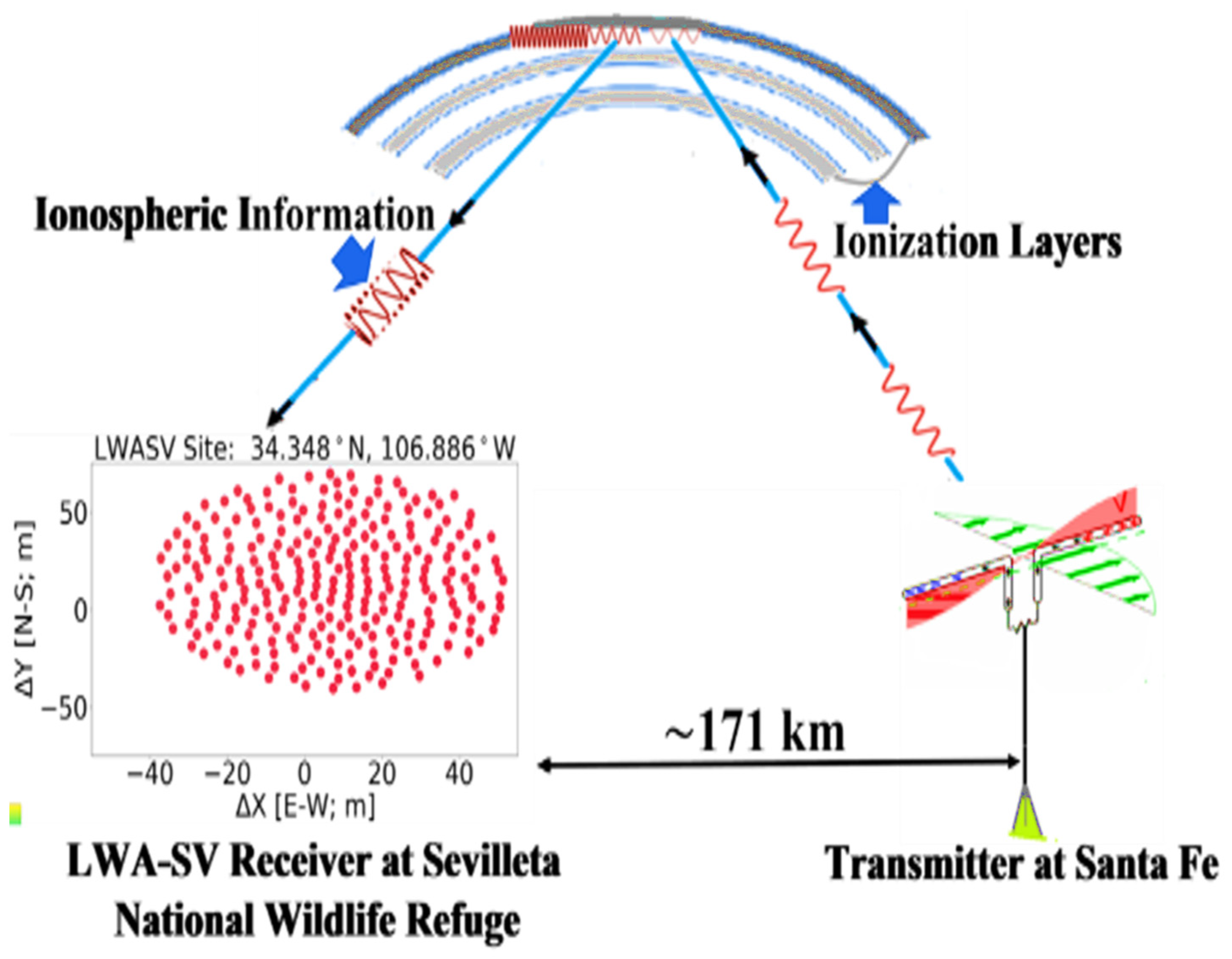
The SDR Earth Imager collects data from the ionosphere by sending radio signals up into the atmosphere at a near-vertical incidence from the Earth’s surface. These radio waves reflect off the ionosphere and return to Earth’s surface where they are imaged using an antenna array camera (
Figure 1).
The phase of the carrier wave was measured using the hardware method. This method uses the quadrature to measure the phase difference between the emitted wave and the received wave. The phase shifts within the phase images show the presence of the waves on/in the ionization layer. The phase shift was determined using the relative phase difference between each pair of antennas at one time. The absolute phase at each antenna could be measured if the transmitter and all the antennae were synchronized.
The phase difference, Δφ, is determined based on the difference in the path length of the radio wave (L) propagating from the transmitter to each receiver in the array, which is expressed as
where
f is the frequency,
λ is the wavelength, and
c is the speed of light.
2.2. LWA-SV and LWA-1 Description of New Mexico Experiments
Datasets were captured at the Long Wavelength Array (LWA)-SV station at the Sevilleta National Wildlife Refuge 34.35°N, 106.89°W [
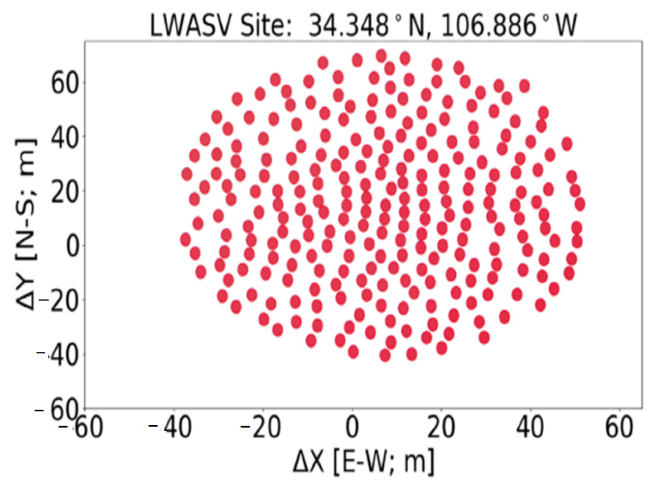
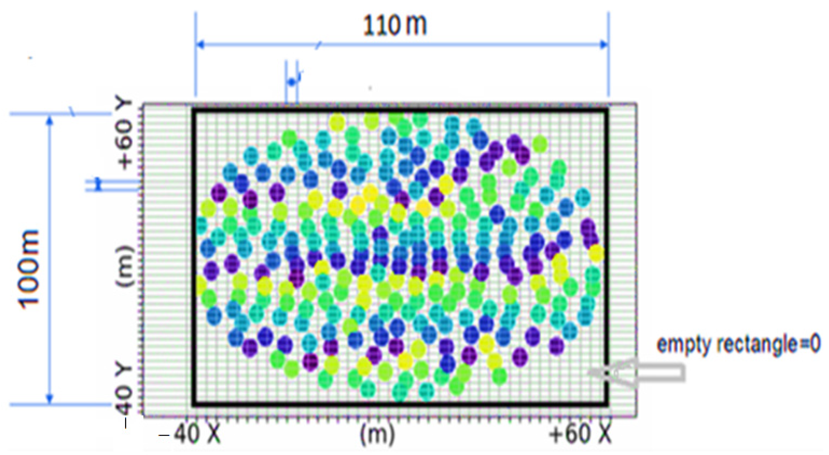
28] LWA-1 station. The LWA-SV and LWA-1 (University Radio Observatory) in central New Mexico captured radio wave frequencies from 3 MHz to 88 MHz, and each array consisted of 256 pairs of dipole-type antennas, while each pair of antennas had orthogonal polarizations on one stand. Antennas of the LWA-SV were arranged in a 110 m by 100 m north–south area distributed in about 100 m of aperture, as seen in
Figure 2 [
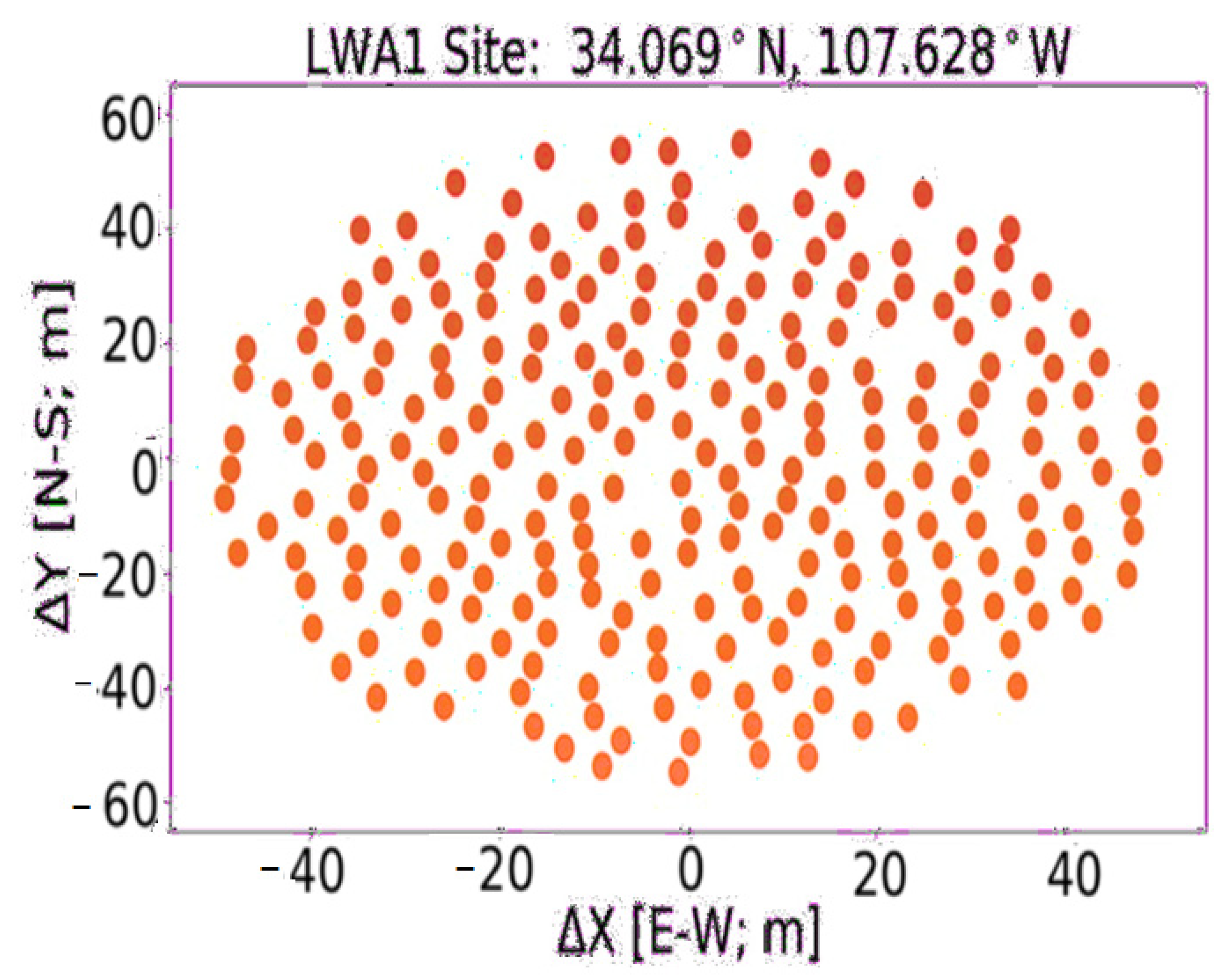
29]. Array geometry of the LWA-1 was within a 100 m (east–west) × 110 m (north–south) elliptical shape, as illustrated in
Figure 3 [
30]. It was designed to produce high-sensitivity, high-resolution images operating over a wide range of frequencies [
31]. Both radio telescope arrays had a minimum of 5 m of separation between the antennas, which allowed for easy access of elements for maintenance purposes and also decreased beam desensitization because of sky noise correlation [
32]. They received a carrier wave after reflection off the ionosphere from a transmitter placed in Santa Fe and transmitted radio waves with frequencies between 3 and 7 MHz. However, only one dataset (5.357 MHz) was analyzed as it had an obvious carrier wave. Transmitter and receiver locations, sent signal, and data specifications utilized during the LWA-SV and LWA-1 experiments are illustrated in
Table 1 and
Table 2 below.
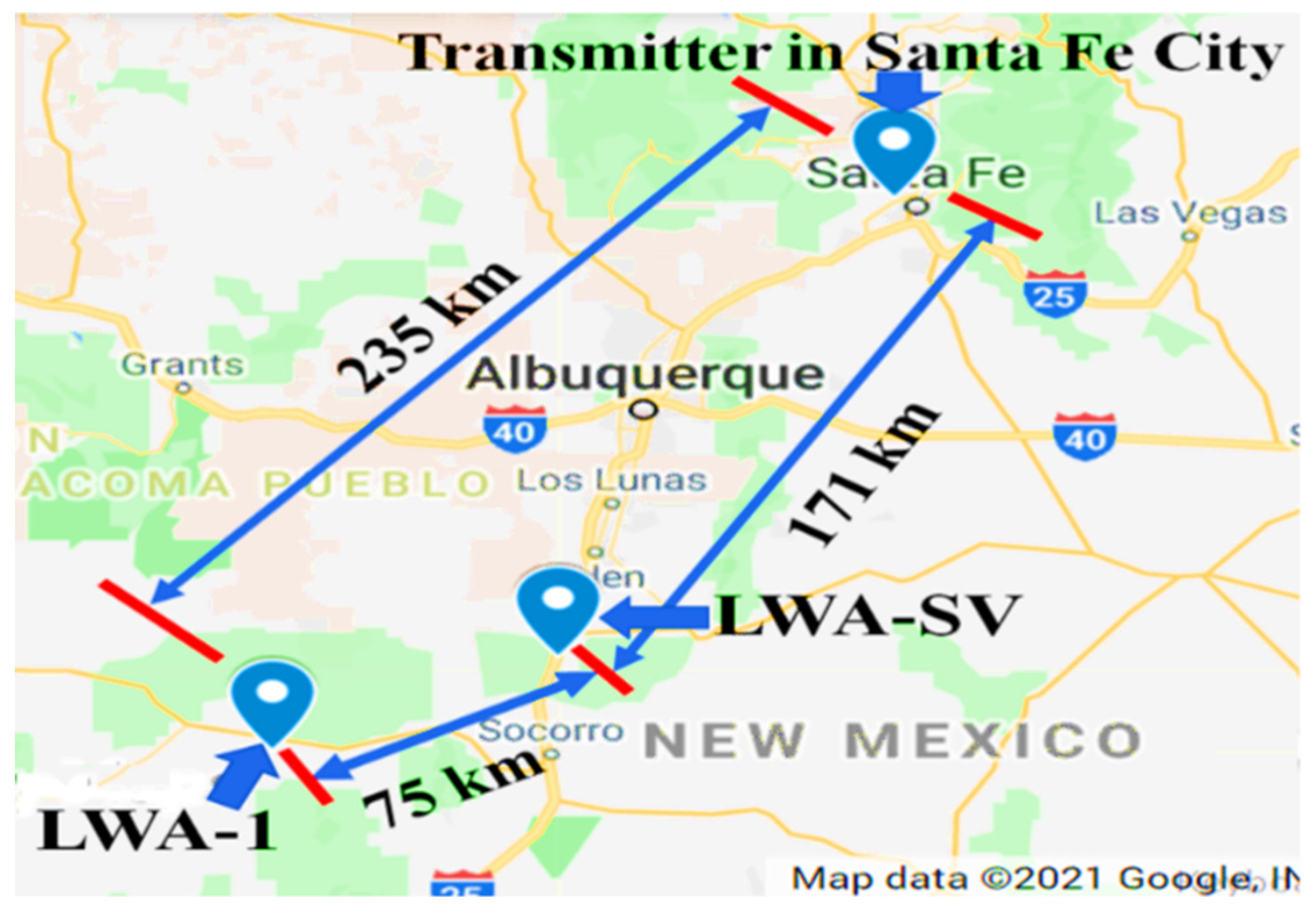
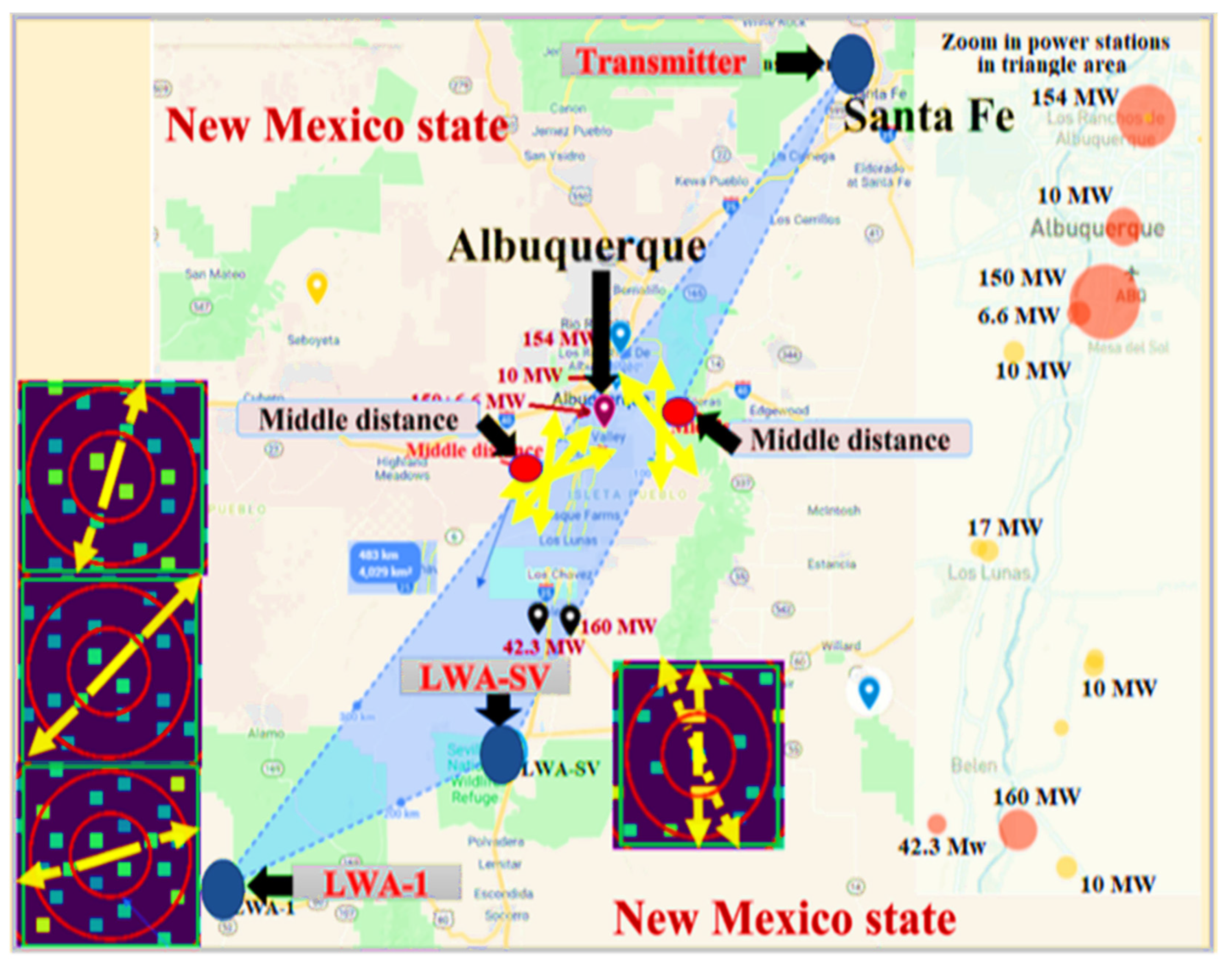
The distance between the Santa Fe transmitter and WA-SV is about 171 km, whereas the LWA-1 station is about 235 km away from the transmitter. The separation between the two stations—LWA1 and LWA-SV—is around 75 km, as shown in
Figure 4 [
30].
3. Results
3.1. LWA-1 and LWA-SV Experimental Results
The LWA Software Library (LSL) was created to manage the specific data formats produced by LWA-1 and LWA-SV and to make them available for basic analysis tools [
33]. A total of about 28 min of each data (LWA-1 and LWA-SV) using a sampling frequency of 100 kHz was obtained by digitally acquiring more than three giga-samples in total. After the initial analysis step, data were found to be consistent throughout the recording time after pre-conditioning (channel selection, noise reduction, etc.). The calculated wavevector (LWA-SV) remained pointed in a north–south direction around 90% of the time, which was in agreement with the physical locations of the transmitter and the receiver array. However, the wavevector for the LWA-1 signals pointed northeast–southwest between 30 to 65 degrees 70% of the time, which showed the effects of the ionospheric disturbances that occurred during the recording time.
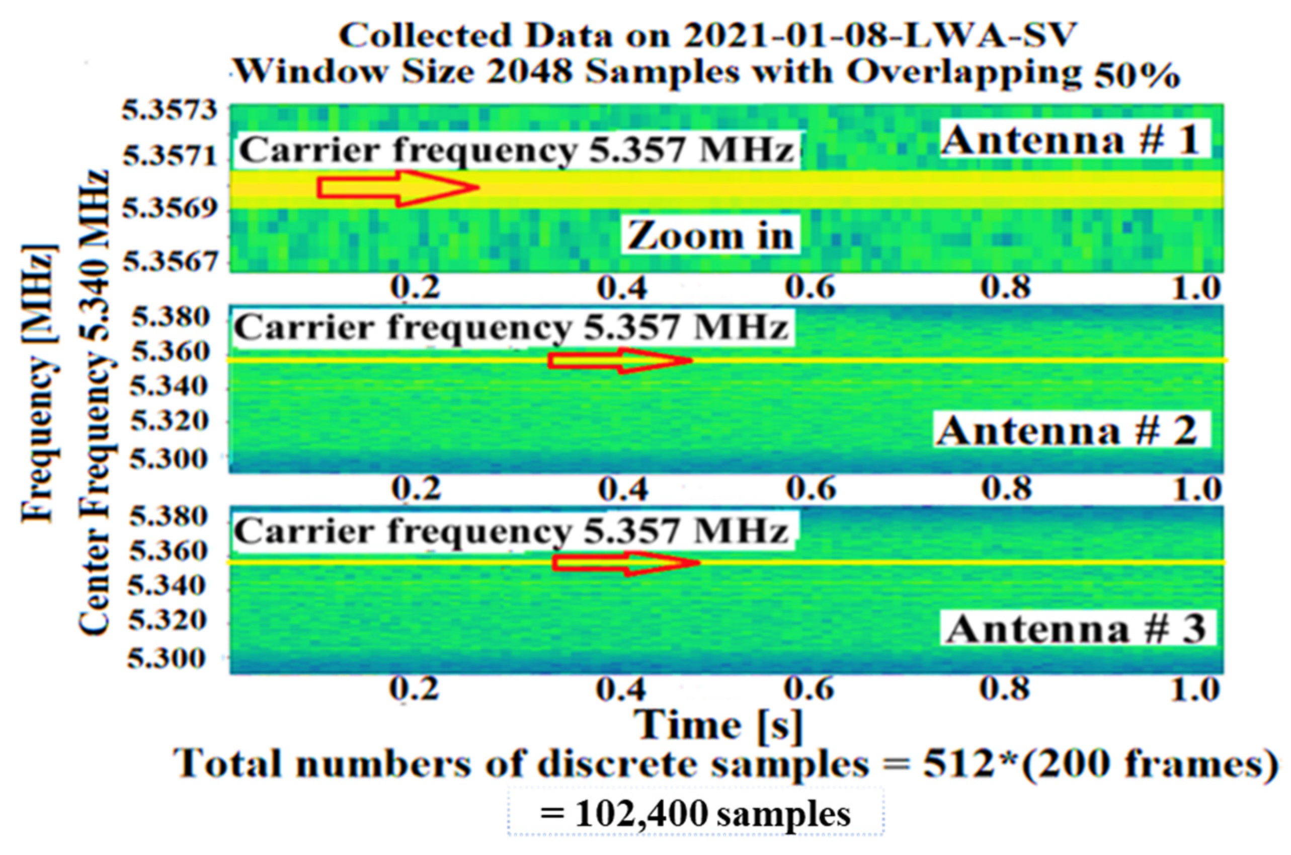
The first step of the data analysis was to represent the data as a waterfall plot.
Figure 5 shows a visual illustration of the transmitted signal strength represented by colors over time and varies with the spectrum of frequencies used to look at the carrier wave extracted from the frequency range.
3.1.1. Carrier Frequency
The carrier frequency (5.357 MHz) worked only as a carrier wave to carry wave information of waves existing in/on the ionosphere to the antenna array. The carrier radio wave propagated through the atmosphere and reflected off the ionization layers. The receiving antennas received the reflected waves at different paths depending on the antenna position. The hardware method used a quadrature to measure the phase of the emitted and received waves to determine their phase difference. The difference in phase of the transmitted and received radio waves was a measure of the phase shift.
3.1.2. Relative Unwrapped Phase
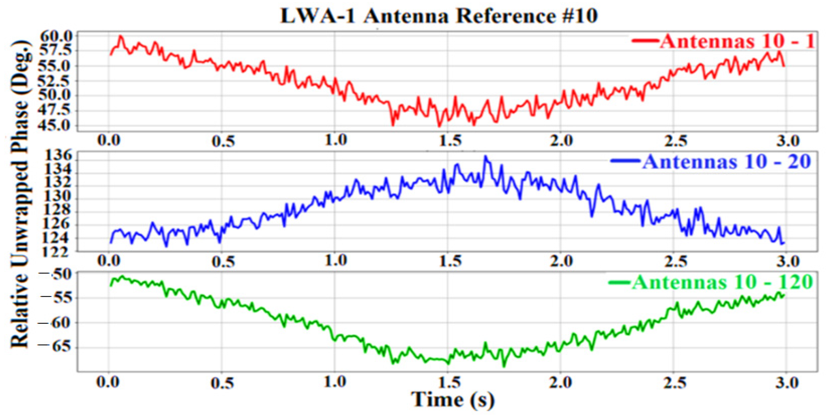
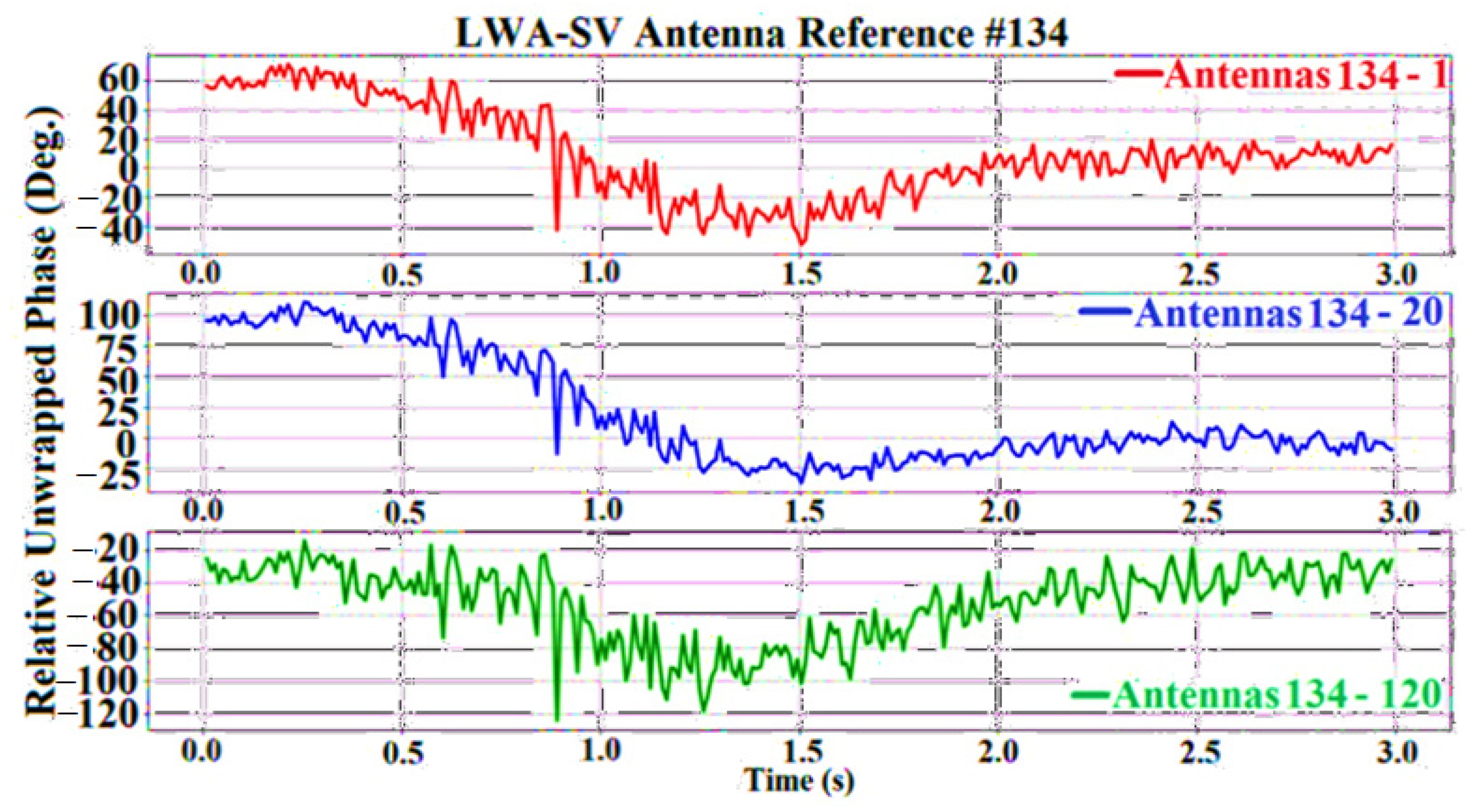
The time difference image was unwrapped, and its relative phase values were determined by taking an antenna close to the center of the LWA-1 and LWA-SV arrays. The relative phase image removed the absolute phase shift that resulted from the tilted carrier wave.
Figure 6 and
Figure 7 show examples of relative unwrapped phase images taken from LWA-1 and LWA-SV during three seconds of collection time. Antenna number 10 is used as a reference for LWA-1 in
Figure 6. Antenna number 134 is used as a reference for LWA-SV in
Figure 7.
3.2. Spatial Phase Image
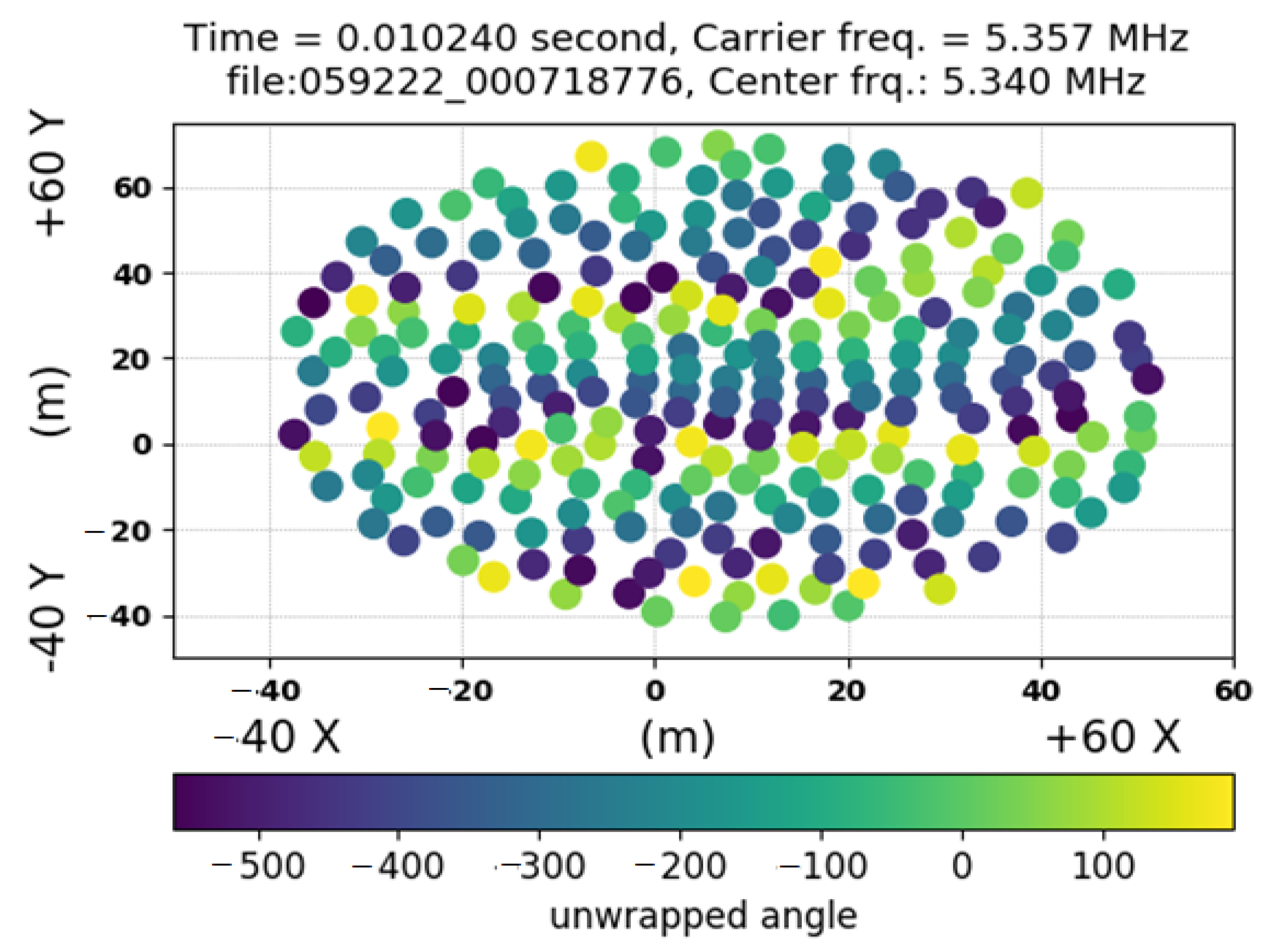
The area of antenna locations in the x-direction and y-direction represents phase image using a relative unwrapped phase, as shown in
Figure 8. The color of the phase image represents the size of the phase shift using unwrapped angles. The positive side illustrates the top of the wave, whereas the negative side shows the bottom side of the wave. The height of a wave represents the amplitude that could be positive or negative. The imaging processing of the relative unwrapped phase was done using a mesh used on the antenna positions and divided into several rectangular shapes. The area (
dx ×
dy) of each cell was around 6 m
2, as depicted in
Figure 9. Each stand had only one relative unwrapped phase, and the pixels outside the image were to zero. Parameters were the center frequency 5.334999 MHz and carrier bin 5.351500 MHz with a sample rate of 100 kHz. The relative unwrapped phases were calculated by taking the stand number 134 of LWA-SV and 10 of LWA-1 as a reference, which were located close to the center of the antenna locations. Polarization zero was chosen as cross-polarizations were provided in the dataset.
A 2D Fourier transformed over the space domain was applied to the relative phase image,
f(
x,
y), to obtain a complex Fourier image,
F(
u,
v) in the spatial frequency domain for each time of data collection,
where
u and
v are the spatial frequencies,
and where
and
are the amplitude and phase distributions of the spatial spectrum given by
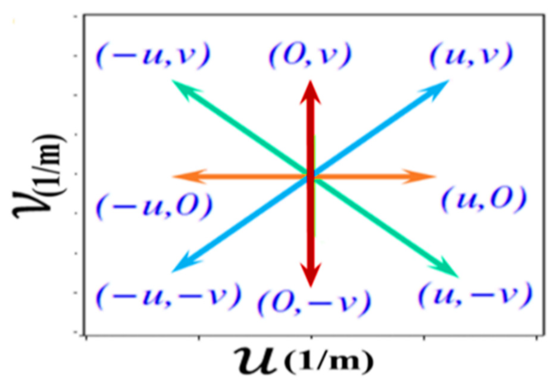
. A 2D Fourier image depicted this symmetry criterion graphically as a succession of symmetric points in the
u and
v plane, as shown in
Figure 10.
3.3. Analysis
The datasets were collected using two locations of receiving antenna array on 8 January 2021. The first frame of LWA-SV started recording at 20:29:20, whereas the first frame of LWA-1 was at 18:00:00. Both datasets lasted around 28 min.
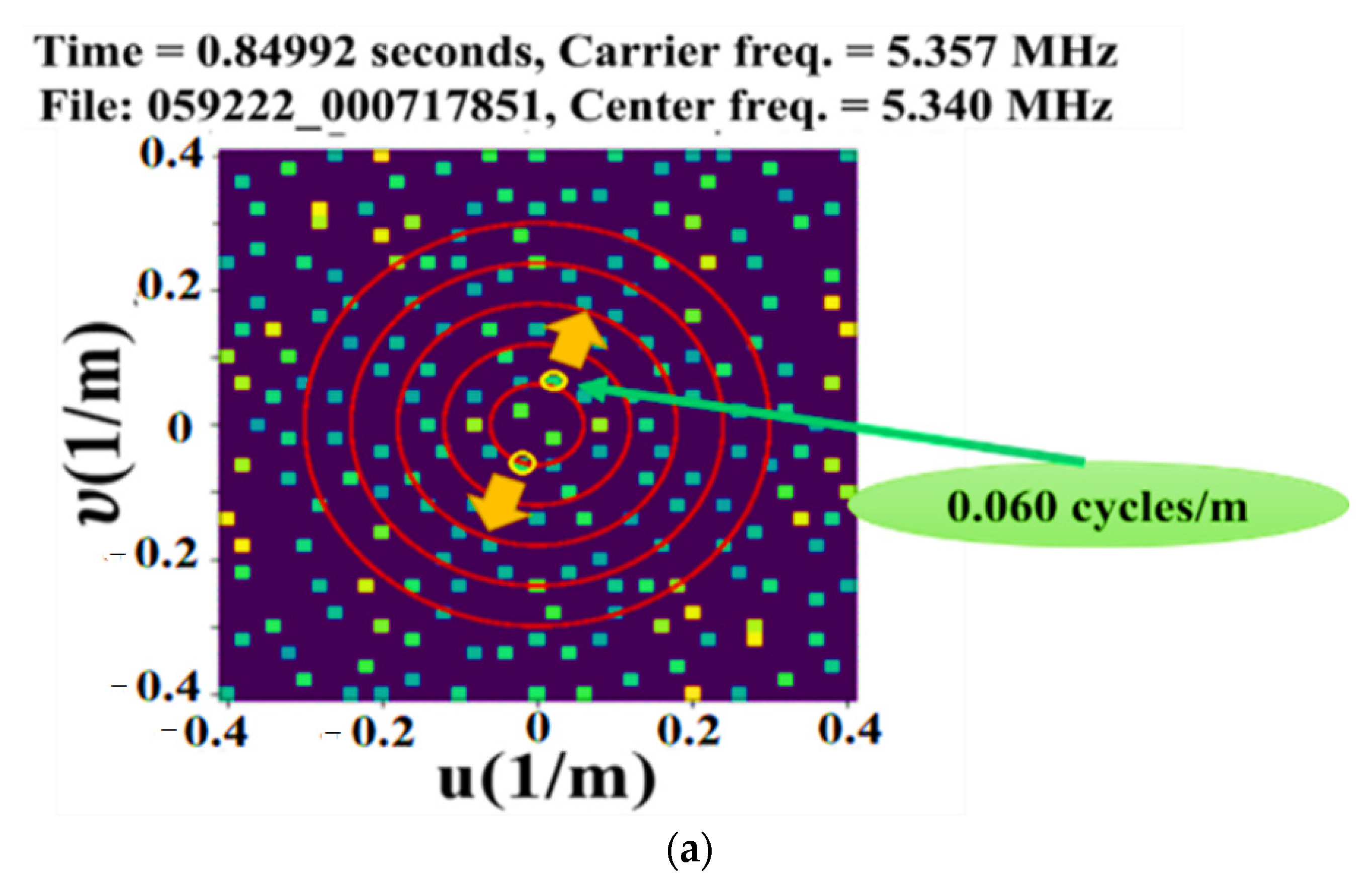
3.3.1. Analysis of LWA—SV Spatial Frequency Result
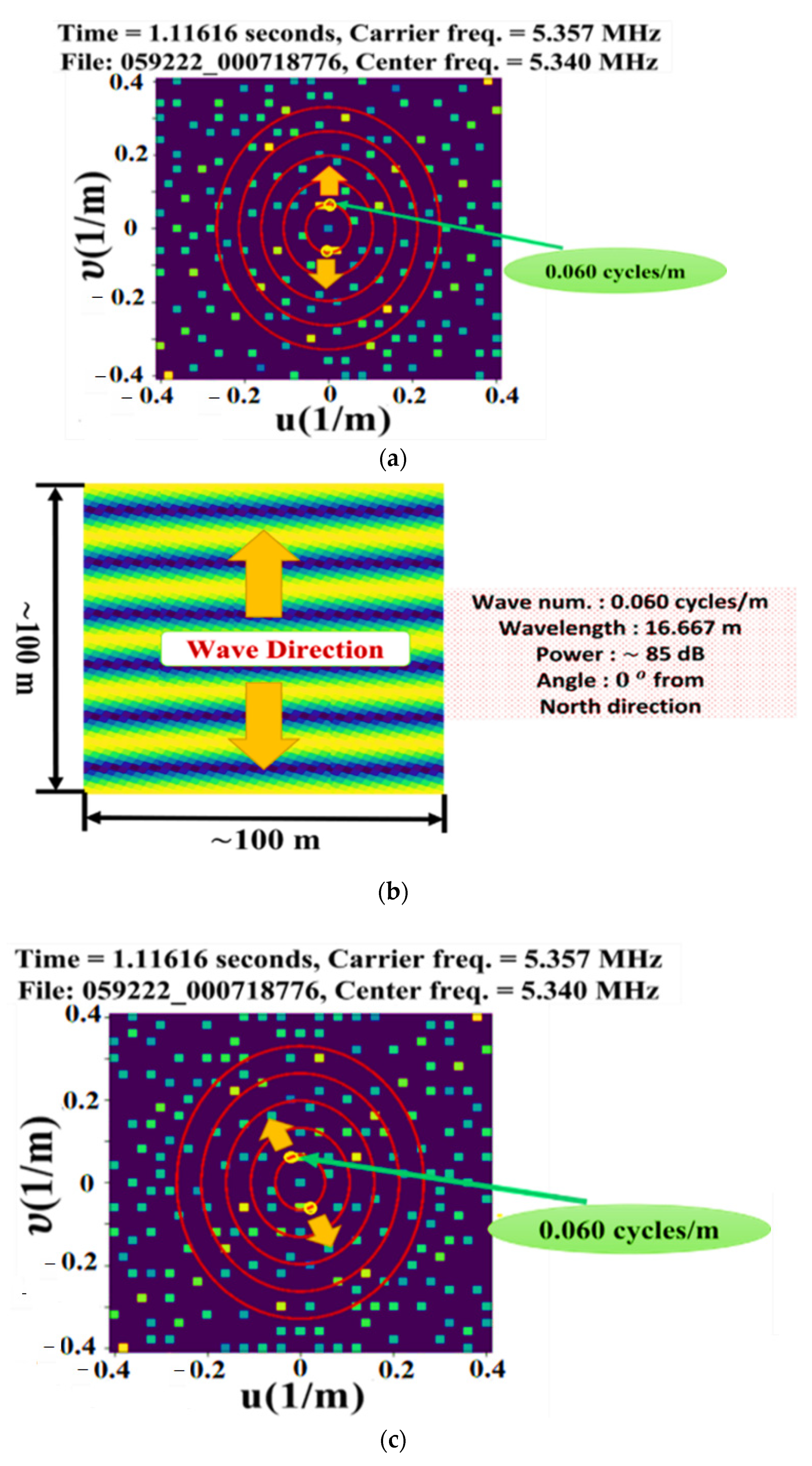
The 2D Fourier image showed many frequency peaks or approximately 170 peaks, as shown in
Figure 11a,c. Each peak represented a set of waves on the ionosphere with its own amplitude, frequency, and wave vector. One pair of peaks located close to the origin had a frequency of 0.06 cycles/m and a wavelength of 16.667 m, which was the largest peak and was studied the most for its possible location of creation. It had a wave vector that sometimes pointed north–south and sometimes slightly tilted from this direction, as shown in
Figure 11. Different time sequences were tested to check the direction of the wavevectors. As a result, the wavevector maintained pointing around 90% of time in a north-south direction, and 10% of time was tilted in a westward direction.
The 2D Fourier images of LWA-SV displayed many spatial frequency peaks (around 170 on one side). The Fourier image shows symmetry sides representing many sets of waves on the ionosphere, as shown in
Figure 11.
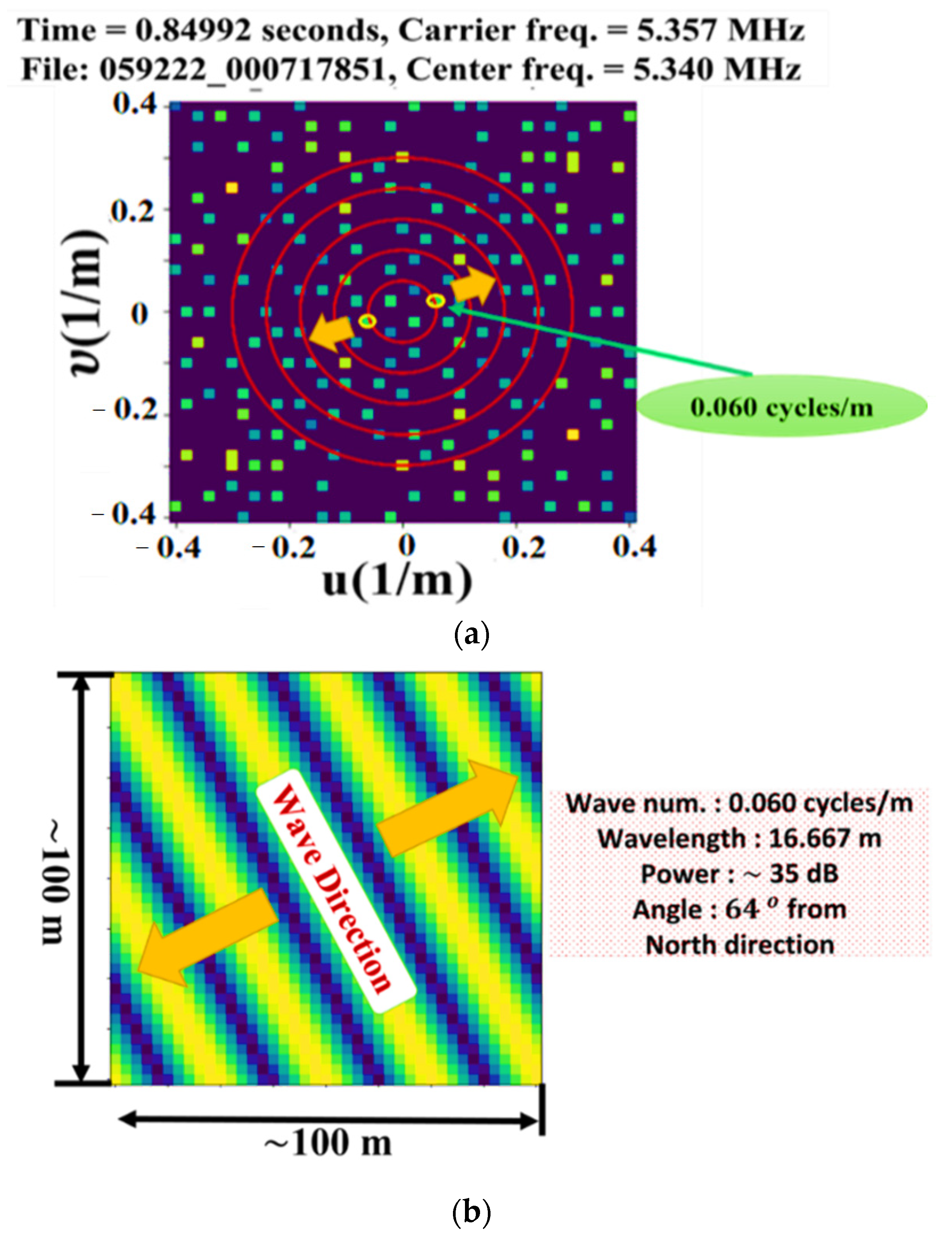
3.3.2. Analysis of LWA–1 Spatial Frequency Results
A 2D Fourier transform space domain was also applied to a relative phase image for LWA-1 to obtain Fourier images for each time of data collection.
The Fourier image reveals symmetrical sides representing numerous sets of waves on the ionosphere, and the 2D Fourier images of LWA-SV exhibited several spatial frequency peaks of about 170 on one side,
Figure 12,
Figure 13 and
Figure 14.
The LWA-1 phase image showed corresponding waves to those seen by LWA-SV. The main Fourier peak was 0.06 cycles/m and was like LWA-SV’s but had a northeast–southwest wavevector instead of a north–south one. The 0.06 cycles/m wave was the largest and strongest peak on both sets of data and was studied the most due to its possible location of creation.
3.3.3. Intersection of the 0.06 cycle/m Wave Vectors from LWA-SV and LWA–1
There are two places on the surface of the ionosphere reflecting the carrier radio wave. They lie mid-way between Santa Fe and LWA-SV and LWA-1, as shown in
Figure 15. Each place had its own set of waves. Their Fourier images nicely revealed the intersection points of their wavevectors that represented the location of the source that created the waves. Possible local wave sources were Albuquerque and its nearby power-generating stations. The two sets of data showed a range of vectors in the LWA-1 Fourier image from around 25 to 60 degrees and from around (0 to 13 degrees) in the LWA-SV image. As a result, the intersection points covered a swath of area between Albuquerque and the power stations.
4. Discussion of LWA-1 and LWA-2 Results
The receiving antenna arrays functioned well as cameras where each antenna represented one pixel in the phase image. Hence, the 256 antennas in the array represented 256 pixels in the phase image. The same carrier wave was transmitted; however, there was a short time difference in collecting the raw dataset between the two LWAs. Their 2D Fourier images showed the same spatial frequency peaks, although not all peaks were similar. The results of the 0.06 cycles/m were the same in terms of their amplitudes, but their wave vectors were different. The wave vectors were different because the direction of the source of the waves was different, i.e., Albuquerque. Albuquerque essentially acted as a point source of disturbance as its waves emanated radially 360 degrees outward. Thus, LWA-1 and LWA-SV saw different wave vectors of the same set of waves. Triangulation using the two sets of wave vectors was used to find the source of the disturbance.
Fourier image analysis showed the presence of ~170 sets of waves that were likely created by both space and Earth disturbing events. There has been some previous research showing a link between man-made Earth disturbing events and ionosphere responses. Such events like these generate waves that have a clear impact on the ionosphere. For example, waves on the ionization layer have been known from ionosondes [
34]. This SDR Atmosphere imager has been shown to provide new information, such as the presence of numerous sets of waves with different amplitudes, frequencies, and wave vectors.
Only one set was studied for its possible location of creation, i.e., the strongest peak had a spatial frequency of 0.06 cycles/m with a wavelength of 16.67 m/cycle. The wavevector of this set of waves at LWA-SV and LWA-1 were the same, and both often pointed in the north–south direction and sometimes slightly tilted off this direction. Based on triangulation of the wavevectors, the location of the possible disturbances that created this set of waves was from the local power generating stations and possibly the grid of their transmission lines around Albuquerque, which is considered a main consumer of power. Time measurements over a 1 s and 3 s period of the 0.06 cycles/m peak had a frequency of 30 Hz. A frequency of 30 Hz could have resulted from the resonances of the 60 Hz in-phase current being transmitted within the power grid around Albuquerque. Several power generators supply Albuquerque and are spatially close to each other; therefore, it is possible that their interference can produce the frequency of 30 Hz found in the measurement.
5. Conclusions
The SDR Earth Imager enabled imaging of the Earth’s ionosphere layer. The wave vector of one set of waves—the strongest with 0.06 cycles/m—was followed in time at both LWA-SV and LWA-1 stations. The most likely sources for this set of waves are the local power generating stations and power usage in Albuquerque, which is a primary consumer of power.
Further investigations are warranted to determine which wave vectors relate to the power of ionospheric waves and local disturbances, such as the power generating stations around Albuquerque.
6. Patents
Patent No: US 10,451,731 B2. Date: 22 October 2019. A Software Defined Radio Earth Atmosphere Imaging system with at least one imager that includes: a radio wave emitter configured to emit a sky wave, a ground wave, and a first line signal; radio wave detectors, including a radio wave detector with a two-dimensional array of radio wave receivers and a radio wave detector for receiving a carrier wave and a ground wave and transmitting a second-time signal; a vector network analyzer, including a Global Navigation Satellite System and at least one synchronization clock; a vector network analyzer in electrical communication with the radio emitter via a first wire and with the radio wave detector via a second wire with the wires used to transmit time signals; a software-defined radio in electronic communication with a vector network analyzer; and a computing device in electronic communication with the vector network analyzer.
Author Contributions
R.S. and R.H. are the main contributors to this research as they applied the idea, followed it up, and analyzed the dataset using a phase imager. P.D. is responsible for setting the time to conduct the experiments and designing the SDR. S.G.T. discussed the approach with us and the derivation of imaging the waves in the ionosphere. The concept of the approach was employed at Dominion Radio Astrophysical Observatory, Penticton, Canada under the supervision of S.H. Finally, all experiments were conducted by W.J. All authors have read and agreed to the published version of the manuscript.
Funding
Natural Science and Engineering Research Council (NSERC) of Canada (RGPIN-2017-03805), and the Ministry of Higher Education and Scientific Research of Libya scholarship.
Data Availability Statement
The dataset is available on Compute Canada Stores.
Acknowledgments
Grants from the Natural Science and Engineering Research Council (NSERC) of Canada, the opportunity to participate in the User Support Program of LWA-1 and LWA-SV at the University of New Mexico are gratefully appreciated. Thank the Ministry of Higher Education and Scientific Research of Libya for their support.
Conflicts of Interest
The authors declare no conflict of interest. We declare that we have no known competing financial interests or personal relationships that could have appeared to influence the work reported in this paper.
References
- Zolesi, B.; Cander, L.R. The General Structure of the Ionosphere. In Ionospheric Prediction and Forecasting; Zolesi, B., Cander, L.R., Eds.; Springer Geophysics; Springer: Berlin/Heidelberg, Germany, 2014; pp. 11–48. ISBN 978-3-642-38430-1. [Google Scholar]
- Moldwin, M. (Ed.) What Is Space Weather? In An Introduction to Space Weather; Cambridge University Press: Cambridge, UK, 2008; pp. 1–16. ISBN 978-0-511-80136-5. [Google Scholar]
- Rishbeth, H. F-Region Links with the Lower Atmosphere? J. Atmos. Sol.-Terr. Phys. 2006, 68, 469–478. [Google Scholar] [CrossRef]
- Piersanti, M.; Materassi, M.; Battiston, R.; Carbone, V.; Cicone, A.; D’Angelo, G.; Diego, P.; Ubertini, P. Magnetospheric–Ionospheric–Lithospheric Coupling Model. 1: Observations during the 5 August 2018 Bayan Earthquake. Remote Sens. 2020, 12, 3299. [Google Scholar] [CrossRef]
- Chum, J.; Liu, J.-Y.; Laštovička, J.; Fišer, J.; Mošna, Z.; Baše, J.; Sun, Y.-Y. Ionospheric Signatures of the April 25, 2015 Nepal Earthquake and the Relative Role of Compression and Advection for Doppler Sounding of Infrasound in the Ionosphere. Earth Planets Space 2016, 68, 24. [Google Scholar] [CrossRef] [Green Version]
- Martines-Bedenko, V.; Pilipenko, V.; Zakharov, V.; Grushin, V. Influence of the vongfong 2014 hurricane on the ionosphere and geomagnetic field as detected by swarm satellites: 2. geomagnetic disturbances. Sol.-Terr. Phys. 2019, 5, 74–80. [Google Scholar] [CrossRef]
- Li, W.; Yue, J.; Yang, Y.; Li, Z.; Guo, J.; Pan, Y.; Zhang, K. Analysis of Ionospheric Disturbances Associated with Powerful Cyclones in East Asia and North America. J. Atmos. Sol.-Terr. Phys. 2017, 161, 43–54. [Google Scholar] [CrossRef]
- Petraki, E.; Nikolopoulos, D.; Nomicos, C.; Stonham, J.; Cantzos, D.; Yannakopoulos, P.; Kottou, S. Electromagnetic Pre-Earthquake Precursors: Mechanisms, Data and Models-A Review. J. Earth Sci. Clim. Chang. 2015, 6, 250. [Google Scholar] [CrossRef] [Green Version]
- Priyadarshi, S.; Yang, J.; Werner, M.; Kryza, M. Ionospheric Perturbations Initiated Due to the Forest-Fire over Greece as a Consequence of Lithosphere-Atmosphere-Ionosphere Coupling. Geomat. Nat. Hazards Risk 2020, 11, 2411–2430. [Google Scholar] [CrossRef]
- Dungey, J.W. Interplanetary Magnetic Field and the Auroral Zones. Phys. Rev. Lett. 1961, 6, 47–48. [Google Scholar] [CrossRef]
- Liu, J.; Wang, W.; Burns, A.; Yue, X.; Zhang, S.; Zhang, Y.; Huang, C. Profiles of Ionospheric Storm-Enhanced Density during the 17 March 2015 Great Storm. J. Geophys. Res. Space Phys. 2016, 121, 727–744. [Google Scholar] [CrossRef]
- Wang, W.; Talaat, E.R.; Burns, A.G.; Emery, B.; Hsieh, S.; Lei, J.; Xu, J. Thermosphere and Ionosphere Response to Subauroral Polarization Streams (SAPS): Model Simulations. J. Geophys. Res. Space Phys. 2012, 117, A07301. [Google Scholar] [CrossRef]
- Zhang, S.-R.; Erickson, P.J.; Zhang, Y.; Wang, W.; Huang, C.; Coster, A.J.; Holt, J.M.; Foster, J.F.; Sulzer, M.; Kerr, R. Observations of Ion-Neutral Coupling Associated with Strong Electrodynamic Disturbances during the 2015 St. Patrick’s Day Storm. J. Geophys. Res. Space Phys. 2017, 122, 1314–1337. [Google Scholar] [CrossRef] [Green Version]
- Liu, J.; Wang, W.; Qian, L.; Lotko, W.; Burns, A.G.; Pham, K.; Lu, G.; Solomon, S.C.; Liu, L.; Wan, W.; et al. Solar Flare Effects in the Earth’s Magnetosphere. Nat. Phys. 2021, 17, 807–812. [Google Scholar] [CrossRef]
- Aa, E.; Zhang, S.-R.; Wang, W.; Erickson, P.J.; Qian, L.; Eastes, R.; Harding, B.J.; Immel, T.J.; Karan, D.K.; Daniell, R.E.; et al. Pronounced Suppression and X-Pattern Merging of Equatorial Ionization Anomalies After the 2022 Tonga Volcano Eruption. J. Geophys. Res. Space Phys. 2022, 127, e2022JA030527. [Google Scholar] [CrossRef] [PubMed]
- Zhang, S.-R.; Vierinen, J.; Aa, E.; Goncharenko, L.P.; Erickson, P.J.; Rideout, W.; Coster, A.J.; Spicher, A. 2022 Tonga Volcanic Eruption Induced Global Propagation of Ionospheric Disturbances via Lamb Waves. Front. Astron. Space Sci. 2022, 9, 871275. [Google Scholar] [CrossRef]
- Harding, B.J.; Wu, Y.-J.J.; Alken, P.; Yamazaki, Y.; Triplett, C.C.; Immel, T.J.; Gasque, L.C.; Mende, S.B.; Xiong, C. Impacts of the January 2022 Tonga Volcanic Eruption on the Ionospheric Dynamo: ICON-MIGHTI and Swarm Observations of Extreme Neutral Winds and Currents. Geophys. Res. Lett. 2022, 49, e2022GL098577. [Google Scholar] [CrossRef]
- Themens, D.R.; Watson, C.; Žagar, N.; Vasylkevych, S.; Elvidge, S.; McCaffrey, A.; Prikryl, P.; Reid, B.; Wood, A.; Jayachandran, P.T. Global Propagation of Ionospheric Disturbances Associated With the 2022 Tonga Volcanic Eruption. Geophys. Res. Lett. 2022, 49, e2022GL098158. [Google Scholar] [CrossRef]
- Pokhotelov, O.; Parrot, M.; Fedorov, E.; Pilipenko, V.; Surkov, V.; Gladychev, V. Response of the Ionosphere to Natural and Man-Made Acoustic Sources. Ann. Geophys. 1995, 13, 1197–1210. [Google Scholar] [CrossRef]
- Astafyeva, E. Ionospheric Detection of Natural Hazards. Rev. Geophys. 2019, 57, 1265–1288. [Google Scholar] [CrossRef]
- Fedorov, E.N.; Mazur, N.G.; Pilipenko, V.A.; Vakhnina, V.V. Modeling ELF Electromagnetic Field in the Upper Ionosphere From Power Transmission Lines. Radio Sci. 2020, 55, e2019RS006943. [Google Scholar] [CrossRef]
- Rothkaehl, H.; Izohkina, N.; Prutensky, N.; Pulinets, S.; Parrot, M.; Lizunov, G.; Blecki, J.; Stanislawska, I. Ionospheric Disturbances Generated by Different Natural Processes and by Human Activity in Earth Plasma Environment. Ann. Geophys. 2009, 47, 1215–1225. [Google Scholar] [CrossRef]
- Obenberger, K.S.; Bowman, D.C.; Dao, E. Identification of Acoustic Wave Signatures in the Ionosphere from Conventional Surface Explosions Using MF/HF Doppler Sounding. Radio Sci. 2022, 57, e2021RS007413. [Google Scholar] [CrossRef]
- Fuller-Rowell, T.J.; Codrescu, M.V.; Moffett, R.J.; Quegan, S. Response of the Thermosphere and Ionosphere to Geomagnetic Storms. J. Geophys. Res. Space Phys. 1994, 99, 3893–3914. [Google Scholar] [CrossRef]
- Burke, W.J.; Huang, C.Y.; Marcos, F.A.; Wise, J.O. Interplanetary Control of Thermospheric Densities during Large Magnetic Storms. J. Atmos. Sol.-Terr. Phys. 2007, 69, 279–287. [Google Scholar] [CrossRef]
- Huang, C.-S. Continuous Penetration of the Interplanetary Electric Field to the Equatorial Ionosphere over Eight Hours during Intense Geomagnetic Storms. J. Geophys. Res. Space Phys. 2008, 113, A11305. [Google Scholar] [CrossRef]
- Garipov, G.; Grigoriev, A.; Khrenov, B.; Klimov, P.; Panasyuk, M. High-Energy Transient Luminous Atmospheric Phenomena: The Potential Danger for Suborbital Flights. In Extreme Events in Geospace; Elsevier: Amsterdam, The Netherlands, 2018; pp. 473–490. ISBN 978-0-12-812700-1. [Google Scholar]
- Bailey, M.A. Investigating Characteristics of Lightning-Induced Transient Luminous Events over South America. Ph.D. Thesis, Utah State University, Logan, UT, USA, 2010. [Google Scholar]
- Malins, J.B.; Obenberger, K.S.; Taylor, G.B.; Dowell, J. Three-Dimensional Mapping of Lightning-Produced Ionospheric Reflections. Radio Sci. 2019, 54, 1129–1141. [Google Scholar] [CrossRef]
- Varghese, S.S.; Obenberger, K.S.; Dowell, J.; Taylor, G.B. Detection of a Low-Frequency Cosmic Radio Transient Using Two LWA Stations. ApJ 2019, 874, 151. [Google Scholar] [CrossRef]
- LWA—About. Available online: http://www.phys.unm.edu/~lwa/abouthome.html (accessed on 2 May 2022).
- Henning, P.; Ellingson, S.W.; Taylor, G.B.; Craig, J.; Pihlström, Y.; Rickard, L.J.; Clarke, T.E.; Kassim, N.E.; Cohen, A. The First Station of the Long Wavelength Array. arXiv 2010, arXiv:1009.0666. [Google Scholar]
- Dowell, J.; Wood, D.; Stovall, K.; Ray, P.S.; Clarke, T.; Taylor, G. The Long Wavelength Array Software Library. J. Astron. Instrum. 2012, 1, 1250006. [Google Scholar] [CrossRef]
- Judd, F.C. Radio Wave Propagation: (HF Bands); Radio Amateur’s Guide; Heinemann: London, UK, 1987. [Google Scholar]
Figure 1.
A transmitter transmitted a carrier radio wave from the Earth, and the carrier radio wave was reflected off the ionosphere captured by receiving antenna arrays.
Figure 1.
A transmitter transmitted a carrier radio wave from the Earth, and the carrier radio wave was reflected off the ionosphere captured by receiving antenna arrays.
Figure 2.
Antenna locations of LWA−SV which show the position of each antenna as a red circle in x and y direction.
Figure 2.
Antenna locations of LWA−SV which show the position of each antenna as a red circle in x and y direction.
Figure 3.
Antenna locations of LWA−1 present the position of each antenna as a red circle in x and y direction.
Figure 3.
Antenna locations of LWA−1 present the position of each antenna as a red circle in x and y direction.
Figure 4.
The distance between the transmitter and both LWA stations as well as the distance between LWA−1and LWA-SV.
Figure 4.
The distance between the transmitter and both LWA stations as well as the distance between LWA−1and LWA-SV.
Figure 5.
A waterfall plot of LWA-SV antenna representing a carrier wave across a frequency range. The color indicates its amplitude demonstrated over time and zooms in for antenna one.
Figure 5.
A waterfall plot of LWA-SV antenna representing a carrier wave across a frequency range. The color indicates its amplitude demonstrated over time and zooms in for antenna one.
Figure 6.
The plot displays an example of the relative unwrapped phases versus time in 3 s for LWA−1.
Figure 6.
The plot displays an example of the relative unwrapped phases versus time in 3 s for LWA−1.
Figure 7.
The graphic shows an example of relative unwrapped phases vs. time in 3 s for LWA-SV.
Figure 7.
The graphic shows an example of relative unwrapped phases vs. time in 3 s for LWA-SV.
Figure 8.
Phase image of antenna locations applying the relative unwrapped phase.
Figure 8.
Phase image of antenna locations applying the relative unwrapped phase.
Figure 9.
Phase image of antenna locations divided into many cells that contain the relative unwrapped phase and the applied Fourier space method mesh.
Figure 9.
Phase image of antenna locations divided into many cells that contain the relative unwrapped phase and the applied Fourier space method mesh.
Figure 10.
Fourier image showing symmetry in two dimensions.
Figure 10.
Fourier image showing symmetry in two dimensions.
Figure 11.
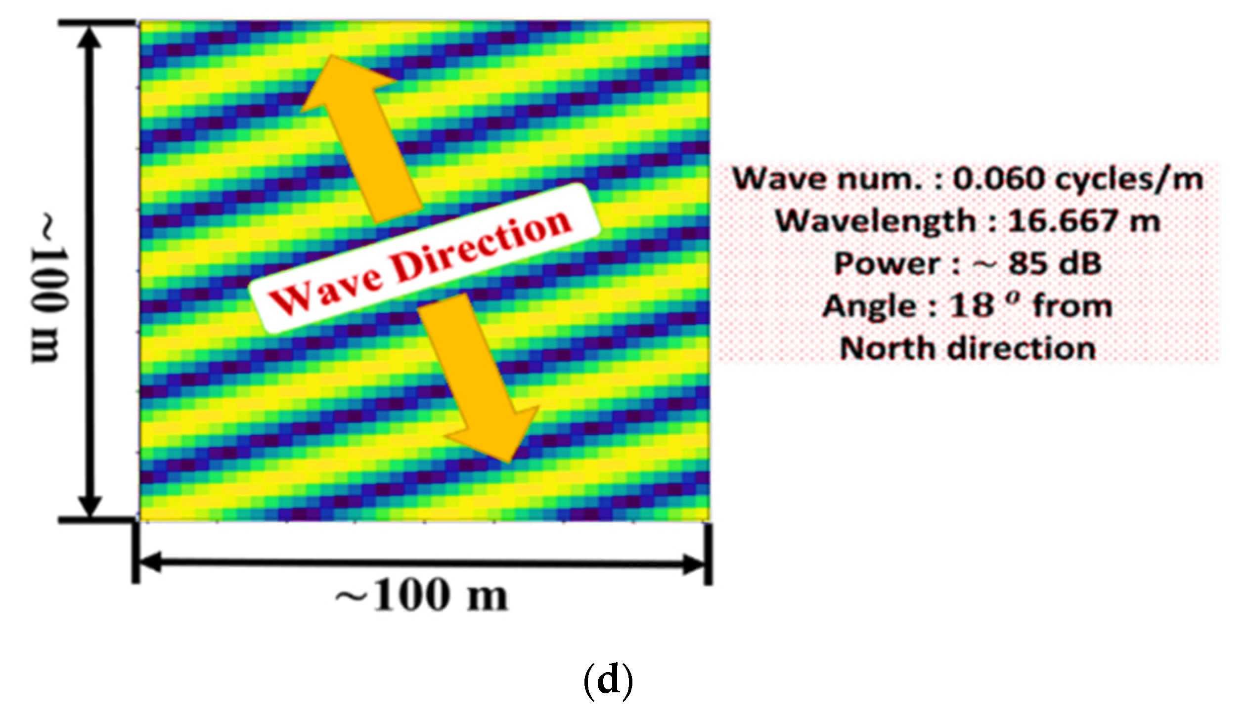
(a) A Fourier image of LWA−SV that shows many peaks which represent sets of detected waves. The the strongest (yellow circle) has 0.06 cycles/m, and the wavevector (yellow arrows) pointing north–south. (b) The inverse Fourier transform (IFT) of (a) revealing the north–south waves. (c) A similar set of waves pointing north–south tilt in a westward direction. (d) The IFT of (c) revealing the tilted waves.
Figure 11.
(a) A Fourier image of LWA−SV that shows many peaks which represent sets of detected waves. The the strongest (yellow circle) has 0.06 cycles/m, and the wavevector (yellow arrows) pointing north–south. (b) The inverse Fourier transform (IFT) of (a) revealing the north–south waves. (c) A similar set of waves pointing north–south tilt in a westward direction. (d) The IFT of (c) revealing the tilted waves.
Figure 12.
(a) A Fourier image demonstrating the wave direction (0.06 cycles/m) (yellow circle) of LWA-1 pointing northeast–southwest with an angle about 30 degrees from the north–south direction. (b) IFT of the spatial frequency with its wave vector.
Figure 12.
(a) A Fourier image demonstrating the wave direction (0.06 cycles/m) (yellow circle) of LWA-1 pointing northeast–southwest with an angle about 30 degrees from the north–south direction. (b) IFT of the spatial frequency with its wave vector.
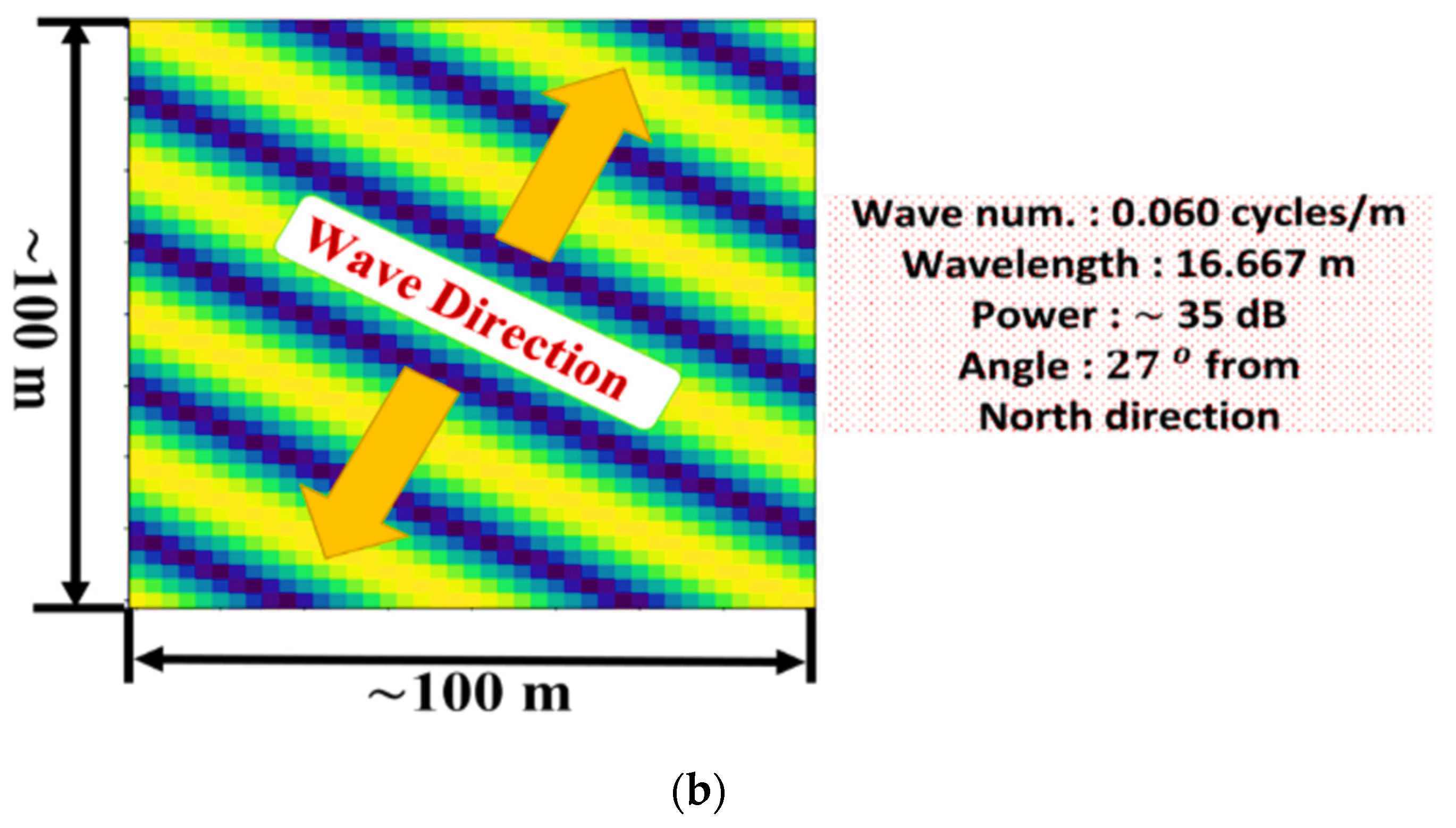
Figure 13.
(a) A Fourier image of LWA-1 data with 0.06 cycles/m displaying a northeast–southwest wave vector direction of ~45 degrees eastward from the north–south direction. (b) Its IFT reveals the set of waves and its wave vector.
Figure 13.
(a) A Fourier image of LWA-1 data with 0.06 cycles/m displaying a northeast–southwest wave vector direction of ~45 degrees eastward from the north–south direction. (b) Its IFT reveals the set of waves and its wave vector.
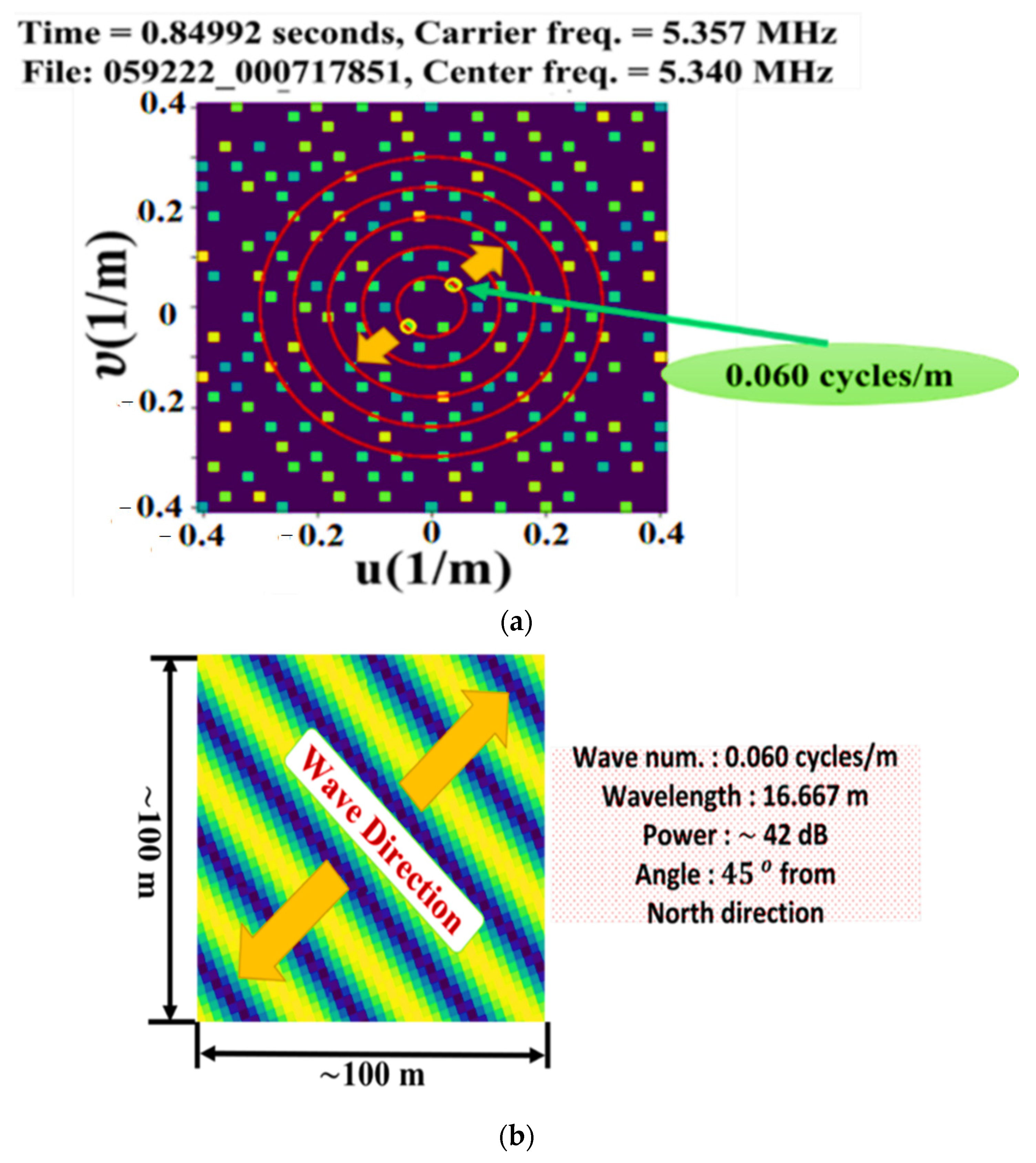
Figure 14.
(a) A Fourier image demonstrating the wave direction (0.06 cycles/m) of LWA-1 with angles about 60 degrees eastward (northeast–southwest) from the north–south direction as well as its IFT in (b).
Figure 14.
(a) A Fourier image demonstrating the wave direction (0.06 cycles/m) of LWA-1 with angles about 60 degrees eastward (northeast–southwest) from the north–south direction as well as its IFT in (b).
Figure 15.
Measured wavevectors at mid-way points (red dots) between Santa Fe and LWA-1 and LWA-SV showing their intersections around Albuquerque and local power generating stations.
Figure 15.
Measured wavevectors at mid-way points (red dots) between Santa Fe and LWA-1 and LWA-SV showing their intersections around Albuquerque and local power generating stations.
Table 1.
Transmitter signal and data set specifications used during the LWA-SV experiment.
Table 1.
Transmitter signal and data set specifications used during the LWA-SV experiment.
| Santa Fe Transmitter (35.71144°N, 106.0084°W) |
|---|
| Date and Time | UT 01 August 2021, 20:29:30 |
| Transmitted Frequency | 5.3570 MHz |
| Mode-Send | CW Tone (Continuous Wave) |
| Receiver LWA-SV (34.348°N, 106.886°W) |
| Center Frequency | 5.33999 MHz |
| Polarization | Zero |
| Date and Time of First Frame | 8 January 2021, 20:29:20 |
| Sample Rate | 100,000 Hz |
| Recorded Time | 1765.895 s |
Table 2.
Transmitter signal and data set specifications used during the LWA-1 experiment.
Table 2.
Transmitter signal and data set specifications used during the LWA-1 experiment.
| Santa Fe transmitter (35.71144°N, 106.0084°W) |
|---|
| Date and Time | UT 01 August 2021, 17:57:32 |
| Transmitted Frequency | 5.3570 MHz |
| Mode-Send | CW Tone (Continuous Wave) |
| Receiver LWA-1 (34.069°N, 107.628°W) |
| Center Frequency | 5.33999 MHz |
| Polarization | Zero |
| Date and Time of First Frame | 8 January 2021, 18:00:00 |
| Sample Rate | 100,000 Hz |
| Recorded Time | 1731.281 s |
| Publisher’s Note: MDPI stays neutral with regard to jurisdictional claims in published maps and institutional affiliations. |
© 2022 by the authors. Licensee MDPI, Basel, Switzerland. This article is an open access article distributed under the terms and conditions of the Creative Commons Attribution (CC BY) license (https://creativecommons.org/licenses/by/4.0/).


