Ore-Waste Discrimination Using Supervised and Unsupervised Classification of Hyperspectral Images

Abstract

Ore and waste discrimination is essential for optimizing exploitation and minimizing ore dilution in a mining operation. The conventional ore/waste discrimination approach relies on the interpretation of ore control by geologists, which is subjective, time-consuming, and can cause safety hazards. Hyperspectral remote sensing can be used as an alternative approach for ore/waste discrimination. The focus of this study is to investigate the application of hyperspectral remote sensing and deep learning (DL) for real-time ore and waste classification. Hyperspectral images of several meters of drill core samples from a silver ore deposit labeled by a site geologist as ore and waste material were used to train and test the models. A DL model was trained on the labels generated by a spectral angle mapper (SAM) machine learning technique. The performance on ore/waste discrimination of three classifiers (supervised DL and SAM, and unsupervised k-means clustering) was evaluated using Rand Error and Pixel Error as disagreement analysis and accuracy assessment indices. The results showed that the DL method outperformed the other two techniques. The performance of the DL model reached 0.89, 0.95, 0.89, and 0.91, respectively, on overall accuracy, precision, recall, and F1 score, which indicate the strong capability of the DL model in ore and waste discrimination. An integrated hyperspectral imaging and DL technique has strong potential to be used for practical and efficient discrimination of ore and waste in a near real-time manner.

1. Introduction

In a mining operation, identification and characterization of the geological features that control the distribution of ore grades and discrimination between ore and waste are essential for optimizing the exploitation process and for production planning. It is essential that any variation in lithology, alteration, and mineralogy exposed to the mine faces be identified and mapped, as it can significantly influence not only the mine’s production performance and its efficiency in terms of produced ore quantity and quality, but also the cost, time, and method of mineral processing. Therefore, using an efficient, rapid, and accurate geological data acquisition approach along with a precise and automated decision-making system is crucial for the mining industry [1,2].

During the extraction of an ore deposit, blasting can dilute the ore grade due to mixing ore and waste in the blasted muckpile. This can be attributed to deposits’ heterogeneities, non-regular mineralization shapes, and contact between ore and waste material. The misclassification of ore/waste can have a significant economic impact on a mining operation [3]. Precise knowledge of ore and waste discrimination at the excavation point is important for minimizing dilution and ore loss. In the conventional approach, the ore zone in the blasted muckpile is subjectively identified by ore-control geologists, based on visual observations and by using blast-induced rock movement data. This process is time-consuming, inaccurate, and can cause safety hazards for mine personnel when walking on a blasted muckpile.

Hyperspectral remote sensing is commonly used in geology for mineral mapping and retrieving surface compositional information for mineral exploration purposes, as well as for lithologic mapping and mine tailings with a focus on acid-generating minerals [4]. Hyperspectral technology is a prime and well-proven phenomenon that characterizes the mineral composition and chemical bonding present in a material and is used to map the characteristics of rocks and minerals. Hyperspectral sensors collect image data simultaneously in hundreds of narrow, adjacent spectral bands. Many materials can be recognized by this method, because the absorption features in their spectra act as unique spectral signatures. Hyperspectral imaging, as a powerful means to discriminate different materials, is an active area of research in mineral identification [5,6]. Hyperspectral ore/waste discrimination based on determining specific spectral features and real-time process monitoring can be a more precise alternative for control of dilution in active mine faces. Pre-concentrating mined ore with hyperspectral-based sorting can reduce mineral processing costs [7,8,9].

Machine learning (ML) and deep learning (DL) techniques provide robust and reliable decision-making tools for analyzing large amounts of sensing data. These techniques have been widely used in different fields of mining [10,11,12]. Using ML and DL, the features of the hyperspectral data can be extracted and learned, which allows different objects to be classified based on their characteristics [13,14]. There are different types of ML techniques that perform well in some specific applications of mineral image classification. Spectral Angle Mapper (SAM) [15,16], a well-known classification mapping technique for remote sensing images, is used in this research. SAM, when used on calibrated reflectance data, is relatively robust against illumination differences and albedo effects and is highly applicable in multitudes of real-life field observations [17]. In n-dimensional hyperspectral space, a pixel vector has both magnitude (length) and angle, measured with respect to the axes that define the coordinate system of the space. SAM identifies pixel spectra only based on angular information [18]. In recent years, DL technology has made outstanding achievements in many fields. Compared with traditional ML image-classification techniques, DL classification reduces the dependence on image resolution, automatically extracts the most effective features by using deep convolution layers in large datasets, and improves the classification speed, which is crucial for ore-waste discrimination [19]. Model structure plays an important role in the training efficiency of a DL model which can lead to high accuracy rates and remarkable performance improvements [20]. U-net [20,21,22] is one such structure used in this study. One of the benefits of a DL model compared to SAM is that when training a DL model, it can be applied multiple times to other spatially and spectrally similar images. In SAM, the whole process should be repeated for every image classification, which can be time-consuming. The k-means [23,24] algorithm is the third classification technique used in this study; it is the most-used unsupervised classification method in the remote sensing field, and is highly efficient. The algorithm is simple and quick to implement, previous knowledge is not required, and unknown classes or patterns in the dataset can be identified. However, the method is computationally intensive; in some cases, accuracy is insufficient, and outliers might get their own cluster. This study compares the application of these three classification algorithms for ore and waste discrimination using hyperspectral image analysis.

A comprehensive review of the strengths and weaknesses of applying DL models to his classification was provided by Paoletti et al. [25]. Some challenges and limitations include dimension, lack of labeled data, and optimization of training parameters. Rangnekar et al. [26] introduced AeroRIT as one of the first large-scale aerial hyperspectral scenes with pixel-wise annotations, and compared the performance of three DL architectures—SegNet, U-Net, and Res-U-Net—for scene understanding and object identification. They concluded that the proposed aerial hyperspectral image would help advance the research in the field with a more complex object distribution.

A limited number of studies have shown the potential of using hyperspectral remote sensing techniques to estimate ore grade classification and to separate ore and waste. Dalm et al. [9] attempted to discriminate between ore and waste samples from an epithermal gold–silver deposit using PLS-DA classifications on hyperspectral imagery of drill core samples. The results were satisfactory with respect to identifying a subset of the waste or sub-economic grade samples, but failed to determine a metric that correctly classified both ore and waste. Natsuo et al. [27] presented mineral-type and grain-size identification using hyperspectral imaging and DL techniques. The hyperspectral data analysis using deep learning identified the mineral species with a high accuracy of over 90%, as compared to RGB data analysis using DL, which had an accuracy of around 30%. Samanta et al. [5] investigated the correlation between copper grade concentrations and mineral spectra absorption parameters using a hyperspectral imaging system. Results showed that the ore grade correlated well with the band depth spectral property. Lypaczewski et al. [28] studied the variability of biotite and white mica mineral chemistry at a gold deposit using hyperspectral data. Results demonstrated that waste could be easily distinguished, but that it would not be possible to determine the exact Au content with this metric. Choros et al. [16] researched the potential of using hyperspectral data for ore grade discrimination using SAM and CNN techniques in a gold deposit. Two approaches were used: ore and waste discrimination as binary classification, and grade classification in four classes from low to high gold grade. In binary classification, CNN (77% overall accuracy) outperformed SAM (60% overall accuracy), but in gold grade classification, the results of both techniques were unsatisfactory, at 22% and 37% for CNN and SAM, respectively.

The main goal of the current study is to compare the performance of the proposed method (a combination of machine learning and deep learning) with two well-known supervised (SAM) and unsupervised (k-means) classification techniques in mineral classification. The focus is to propose an innovative and automated approach to real-time mapping of ore and waste classification with high accuracy.

Our study represents an original contribution to the design and evaluation of machine learning techniques for ore and waste discrimination using hyperspectral images taken from drill core samples. Several of the methods presented here have been reported in the literature, but the combination of the methods adopted and evaluated in this paper, using data from a silver deposit, are novel. Our dataset is an original hyperspectral image of significant size taken from multiple core samples from a silver mine that were labeled by geologists as ore material and waste material. Our approach addresses the challenge presented by the mismatch between the core-level resolution of the ground truth provided by geologists, and the pixel-wise resolution needed to train an established image segmentation deep neural network (specifically, the ENVI implementation of U-Net). Our work includes a detailed evaluation (considering core- and pixel-level resolutions) of the ENVI deep learning module results obtained after training with SAM generated labels against both supervised (SAM) and unsupervised (k-means) machine learning techniques. Finally, our study takes care to avoid data leaks between training and test data (see [29] and our discussion in Section 3.2.1).

In this study, a silver deposit is used as a case study where silver mineralization is related to the hydrothermal system. As strong absorption features of hydrothermal alteration minerals appear in the shortwave near-infrared region, SWIR (900–2500 nm). Employing the SWIR data for geological mapping applications has been demonstrated in different studies [30,31,32]. In this paper, 256 SWIR spectral bands of hyperspectral data, obtained from drill cores, were used as labeled data for the deep learning model.

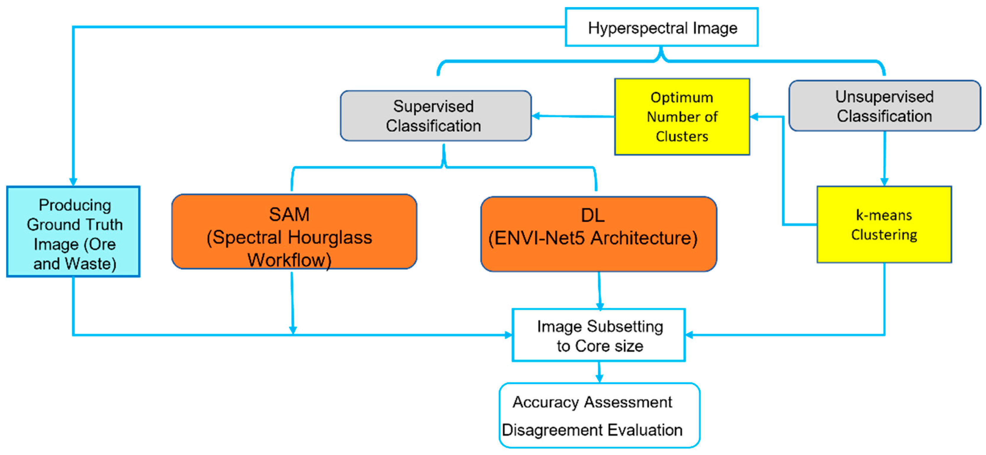
2. Materials and Methods

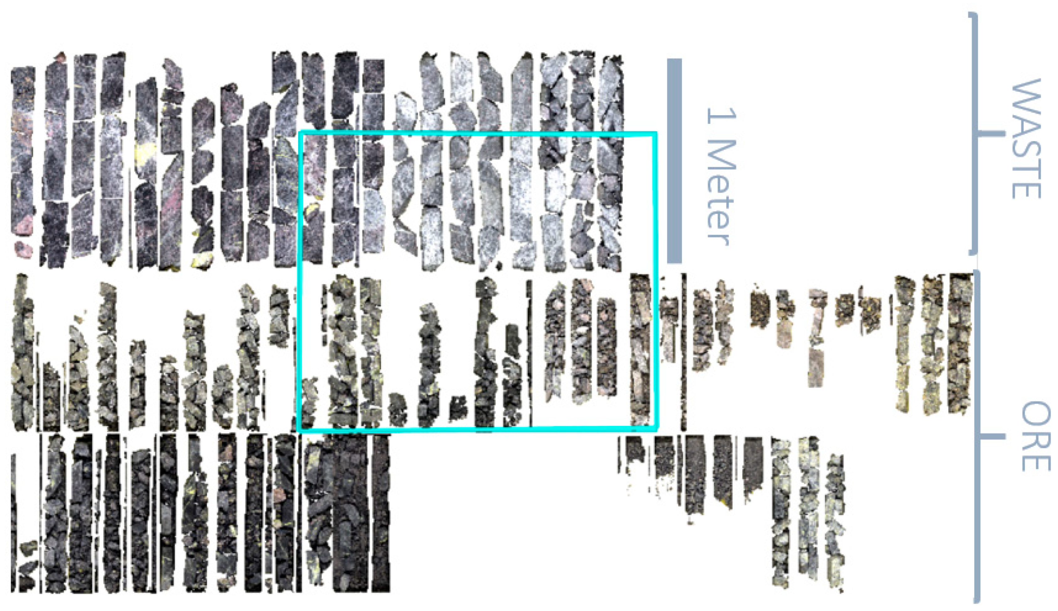
2.1. Dataset

The dataset used in this study includes several meters of drill cores (~16 m in total) from a silver deposit labeled by geologists as ore material and waste material. Samples were collected from five drill holes. Three holes were classified as ore, and samples from these holes were placed into 14 ore core boxes; two holes were classified as waste, and the samples from these holes were put into 5 waste core boxes. The ore drill core samples show silicic and propylitic alterations, while the waste core samples are mostly unaltered igneous porphyry cut by minor veins of epidote and chlorite.

Waste and ore cores were scanned by a hyperspectral scanner capturing range of reflectance from the visible near-infrared to the shortwave infrared. The scanner had an integration time of 2 ms with a spectral resolution of 6 nm and spatial resolution of 3 pixels/mm. As strong absorption features of hydrothermal alteration minerals appear in the shortwave infrared region, and hydrothermal alteration includes the main mineralization in the deposit, only the SWIR data were processed, in order to avoid complicated processing. The size of the dataset is 6,494,400 pixels (10,560 by 6150), and each pixel contains 256 bands. Note that the size of the dataset in this study is significantly larger than all the popular hyperspectral image segmentation benchmark datasets, including the largest benchmark that we referenced earlier, AeroRIT [26], which has 7,842,675 pixels (1973 by 3975). Figure 1 shows the hyperspectral near-infrared image of the scanned drill core samples. The blue rectangle indicates the area used for deep learning training, which will be discussed below in the section on deep learning classification. The scanner had an integration band color as follows: red, 2163 nm; green, 2200 nm; and blue, 2350 nm.

Samples were geochemically and petrographically analyzed to acquire more information about sample content. Silver content and whole-rock geochemistry were acquired from aliquots of the ore material (ore portion of Figure 1) and sent to a laboratory for assay. Geochemical analyses of elemental abundances were acquired using X-ray Fluorescence (XRF) and Inductively Coupled Plasma Mass Spectroscopy (ICP-MS); fire assay was used to measure silver concentrations. Petrographic analyses using both transmitted and reflected light microscopy were also performed. Petrography of the samples shows chlorite and epidote alteration within the ore material, with calcite and quartz stockwork veins. Sulfide mineralization of pyrite, chalcopyrite, sphalerite, and galena were also observed. Sulfide textures were found as blebby and disseminated. Silver mineralization was identified as hosted within sulfur-bearing minerals. Native silver was not observed within any samples. Results of the silver assay display a wide distribution of silver content, ranging from <1 ppm to 3630 ppm. The ICP analysis showed that silver content is correlated to zinc, lead, and silica content. This is likely a result of the silver forming in an epithermal-style deposit. The overall trend shows increasing silver content with increasing silica content, as well as with increasing zinc content.

2.2. Methodology

In this study, the ability to use hyperspectral data to discriminate between ore and waste rock samples was investigated using the deep learning method (DL) and Spectral Angle Mapper (SAM) as supervised classification techniques, and k-means as a well-known unsupervised classification technique, as shown in the workflow illustrated in Figure 2. The elbow method was used to find the optimum number of classes for classification. In the SAM model, the hyperspectral data were processed using spectral hourglass workflow. The ENVINet5 architecture was used as the DL classification model in this study. A ground truth image of ore and waste of the same size was produced from HS data to evaluate the mentioned techniques’ performance. This image was based on the field geologist’s interpretation in which each box containing core samples was labeled as ore or waste. To avoid background effects in evaluation analysis, classification results were decomposed for each core sample by numbering the samples. Accuracy assessment and disagreement evaluation on all three classification techniques were calculated for each core beyond the training area (52 cores).

2.2.1. Spectral Angle Mapper

Spectral Angle Mapper (SAM) is the exclusive spectral similarity measure used in remote sensing. It is a whole-pixel technique that is primarily used for target detection. SAM, a supervised classification method, uses an n-dimensional angle to match pixels to reference spectra. The reference spectra can be either laboratory or field spectra, or extracted from the image. The spectral similarity between two spectra will be determined by calculating the angle between a spectral pixel in the image and a reference spectrum. Smaller angles represent closer matches to the reference spectrum [33].

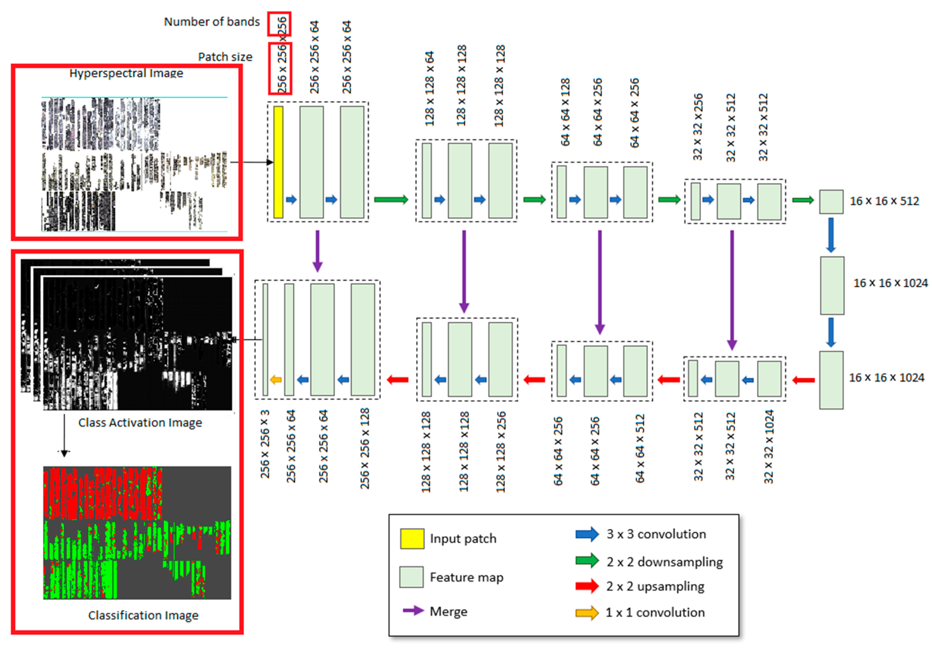
2.2.2. Deep Learning

As mentioned in the introduction, the current study aims to accelerate real-time mapping of ore and waste classification with high accuracy. Past studies have shown that the deep learning method is useful for achieving image-based classification. This study uses ENVI-Net5 as a deep learning module for classification. The ENVI deep learning module used in this paper is considered more convenient compared to other approaches. ENVI deep learning requires no programming, is simple to apply, and has a low error rate. In addition, it can be applied to the identification of ore and waste in large areas with complex conditions. Programming-based deep learning provides a more flexible yet complex approach to mapping than the software-based approach, which is rigid, fast, and does not require coding [34].

The architecture that ENVI deep learning uses, called ENVI-Net, is an encoder-decoder convolutional network that classifies every pixel in the image, based on the U-Net architecture developed by Ronneberger et al. [35]. The input of ENVI-Net is a patch with the entire extent of the training data, and the model can learn based on the pixels specified in the patch. The output is an activation image where the pixel values range from 0 to 1, and a classification image with labels as values. Based on an initial guess in the first training pass, the model generates a class activation raster and compares it to the label raster. The model learns to optimize its weights through a loss function to improve its accuracy. However, data are not passed through training all at once. Instead, square patches of a given size are extracted from the label raster and are used for training a few at a time [36].

The architecture of the model is characteristic of U-Net, which has 5 levels and 27 convolutional layers. Figure 3 shows standard architecture using in the ENVI package. Modified parts based on our dataset are highlighted by red rectangles. Each level represents a different pixel resolution in the model, and the image is downsampled and upsampled four times. Downsampling (Encoder) gradually reduces the image size while the depth gradually increases. Upsampling, in which the expansion path (Decoder) applies transposed convolutions along with regular convolutions, gradually increases the size of the image, while the depth gradually decreases. The Encoder path follows the typical architecture of two 3 × 3 convolutions each, followed by a rectified linear unit (ReLU) and a 2 × 2 max pooling operation with stride 2 for downsampling. The number of feature channels is doubled for each downsampling step. The Decoder path is the mirror of the Encoder path. Concatenation (merging) of feature maps helps give localization information. The last layer contains a 1 × 1 convolution used to map each component feature vector to the desired number of classes (three in this study). Training involves repeatedly exposing the label raster to a model. Over time, the model will learn to translate the spectral and spatial information in the label raster into a class-activation raster that highlights the features it was shown during training [35]. The architecture of the model is described in detail in [36,37]. ENVI deep learning, using the TensorFlow pixel classification tool, allows one to train a model once and apply it multiple times elsewhere on the same image, or on others that are spatially and spectrally similar [35].

2.2.3. K-Means

k-means is the most widely used unsupervised learning algorithm in remote sensing fields. It partitions data into k clusters such that data points in the same cluster have the most similarities with each other and the most differences from data points in the other clusters. Initial cluster centers are randomly chosen for each cluster, and then each pixel is assigned to the nearest centroid based on the Euclidean distance. The k-means algorithm is an iterative process. After assigning pixels to clusters, it tries to recalculate each centroid as the arithmetic mean of all samples in the cluster. The procedure is repeated until the convergence criterion is met [38].

The weakness of the k-means algorithm is the determination of the number of clusters. There are some methods to deal with this issue; the elbow method is the most popular. The elbow method is a visual method which plots the variance (within-cluster sum of squared errors, SSE) against the number of clusters. The most extreme difference-forming point in the trend of the plot (the angle of the elbow) shows an optimum number of clusters [39,40].

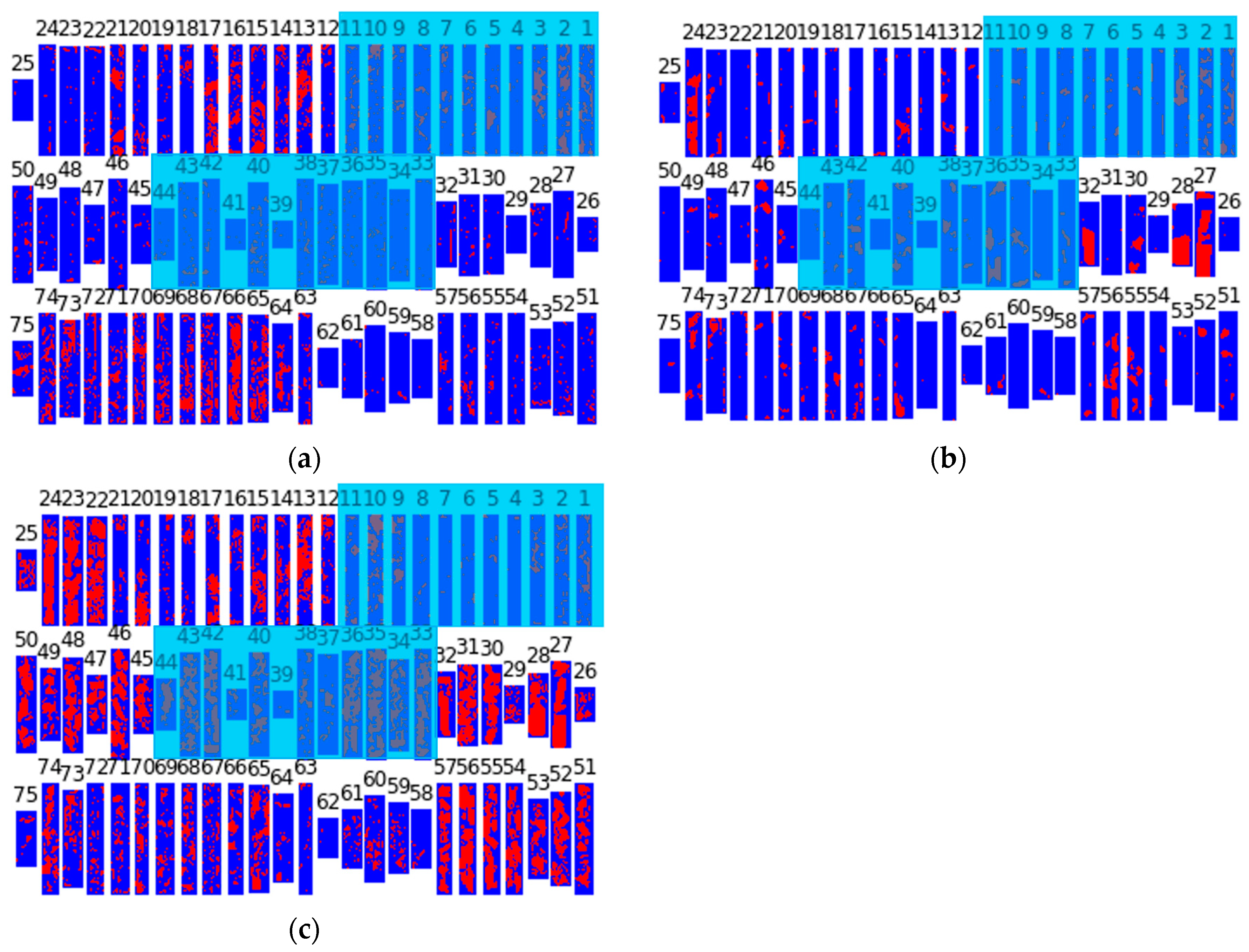
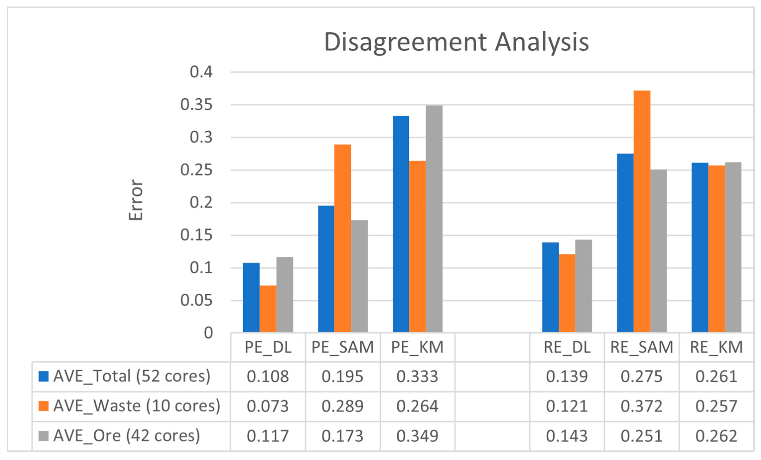
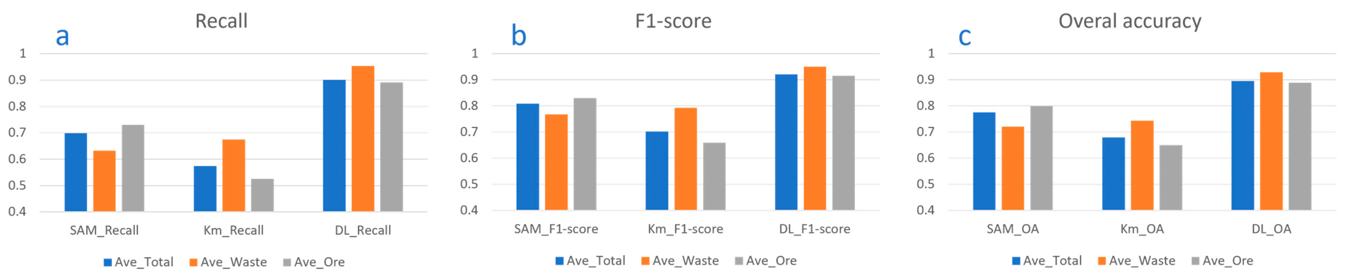
2.2.4. Accuracy Assessment and Disagreement Analysis

Deep learning models were monitored for loss and accuracy during the training process. To maximize the efficiency of the model, the loss should be minimized. ENVI-Net5 refers to the energy function, which is a combination of pixel-wise softmax over the final feature map with the cross-entropy loss function. Detailed information can be found in [35].

There are different methods to evaluate the performance of classifiers. Pixel Error (PE), a type of disagreement analysis, is the simplest way of evaluating a segmentation. It counts the number of pixels where the classified (predicted) image disagrees with (is not the same as) the labeled image. This can also be written as the squared Euclidean distance |L − L*|, where L is a binary classified image and L* is a binary labeled image. A distance greater than 0 is a pixel with disagreement. Rand Error (RE), another measure of disagreement, is the frequency of pixel pairs belonging to the same region (label) in one segmentation but no other (Equations (1) and (2)). Rand error is expressed with the following equations:

$$\mathrm{RE}=1-\mathrm{RI}$$

(1)

$$\mathrm{RI}=\frac{\mathrm{a}+\mathrm{b}}{\left(\begin{array}{c}\mathrm{n}\\ 2\end{array}\right)}$$

(2)

where RI is Rand Index, a well-known measure of the similarity between two data clusters.

Given two segmentations, A and B, of an image L with n pixels, there are:

• a, the number of pairs of pixels in L that are in the same object in A and in the same object in B (i.e., they have the same label)
• b, the number of pairs of pixels in L that are in different objects in A and in different objects in B (i.e., they have different labels) [41].

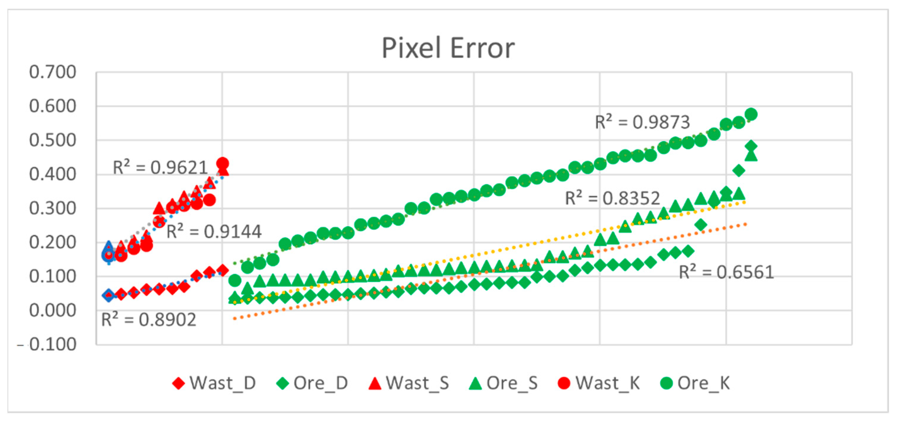
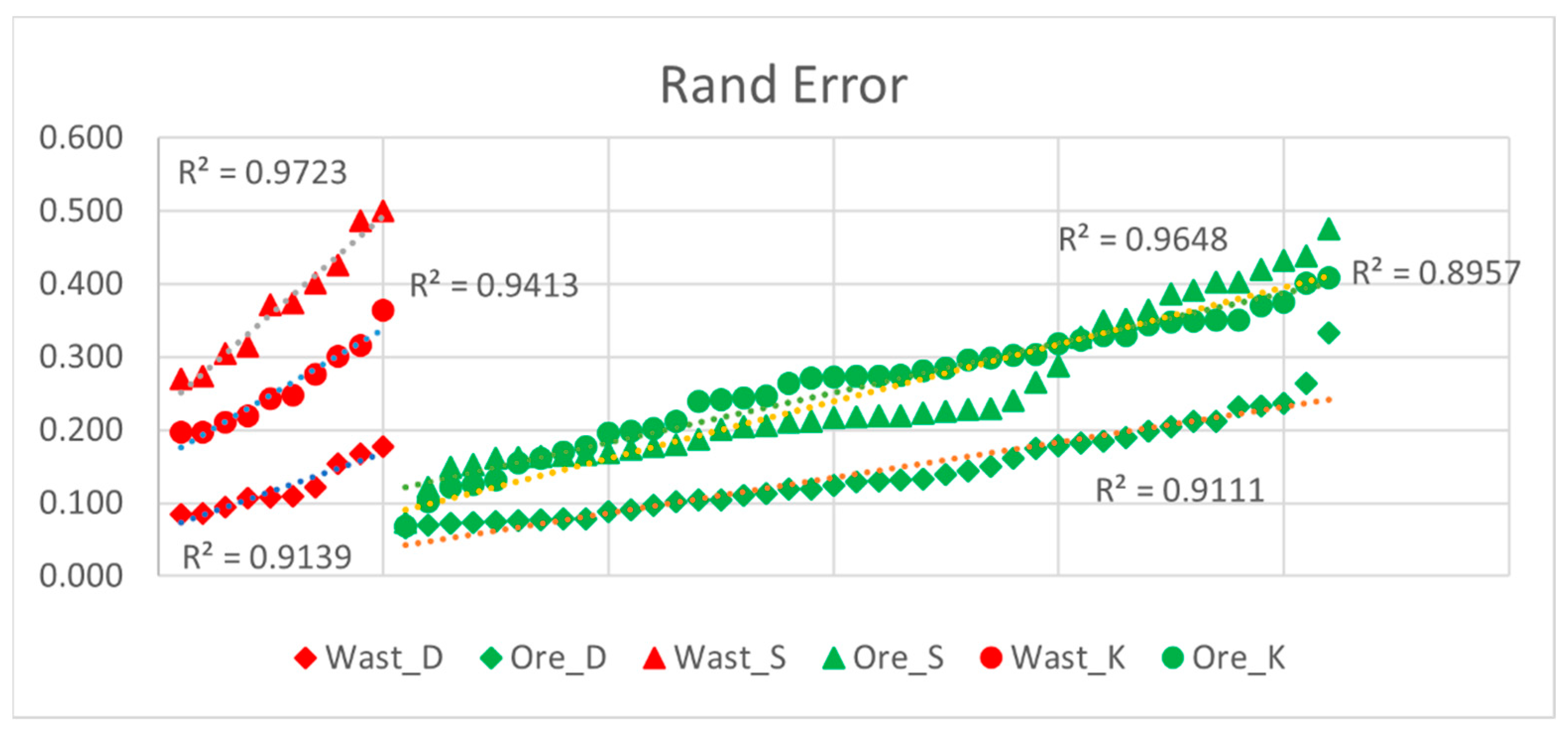
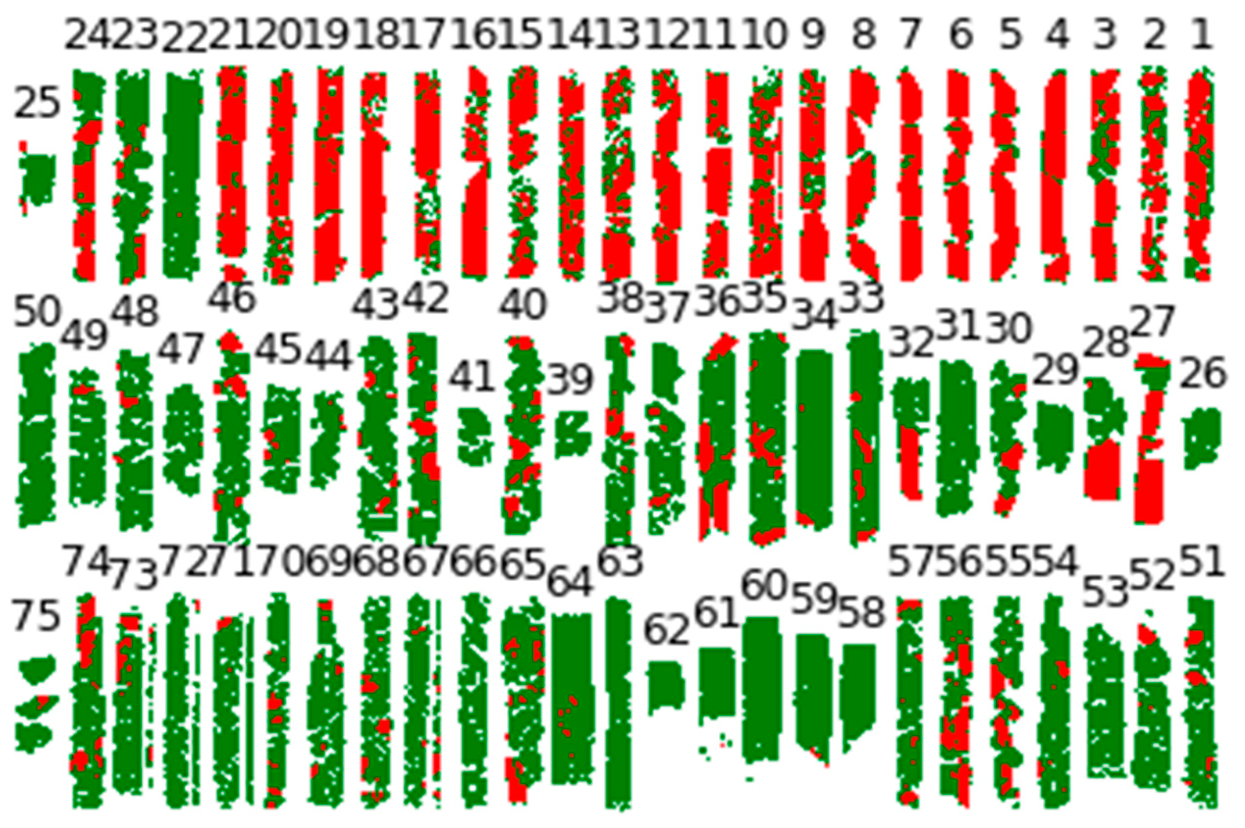
The evaluation indices include loss, accuracy, precision, recall, and F1 score, and are used to verify the test dataset. The loss is a unitless number, which indicates the degree of matching between the classifier and the verification training data; a value of 0 indicates a perfect fit. Overall accuracy is the sum of the percentages of pixels correctly identified in different classes. The precision indicates the proportion of correctly predicted pixels to all positive predictions. The recall refers to correctly predicting the proportion of positive pixels to all actual positive pixels. The F1 score is a harmonic combination between precision and recall. Further information on the evaluation indices can be found at [34,42,43].

In this study, disagreement analysis (PE and RE) and assessment indices are used to evaluate the performance of classifiers. The assessment indices include overall accuracy, precision, recall, and F1 score.

3. Results

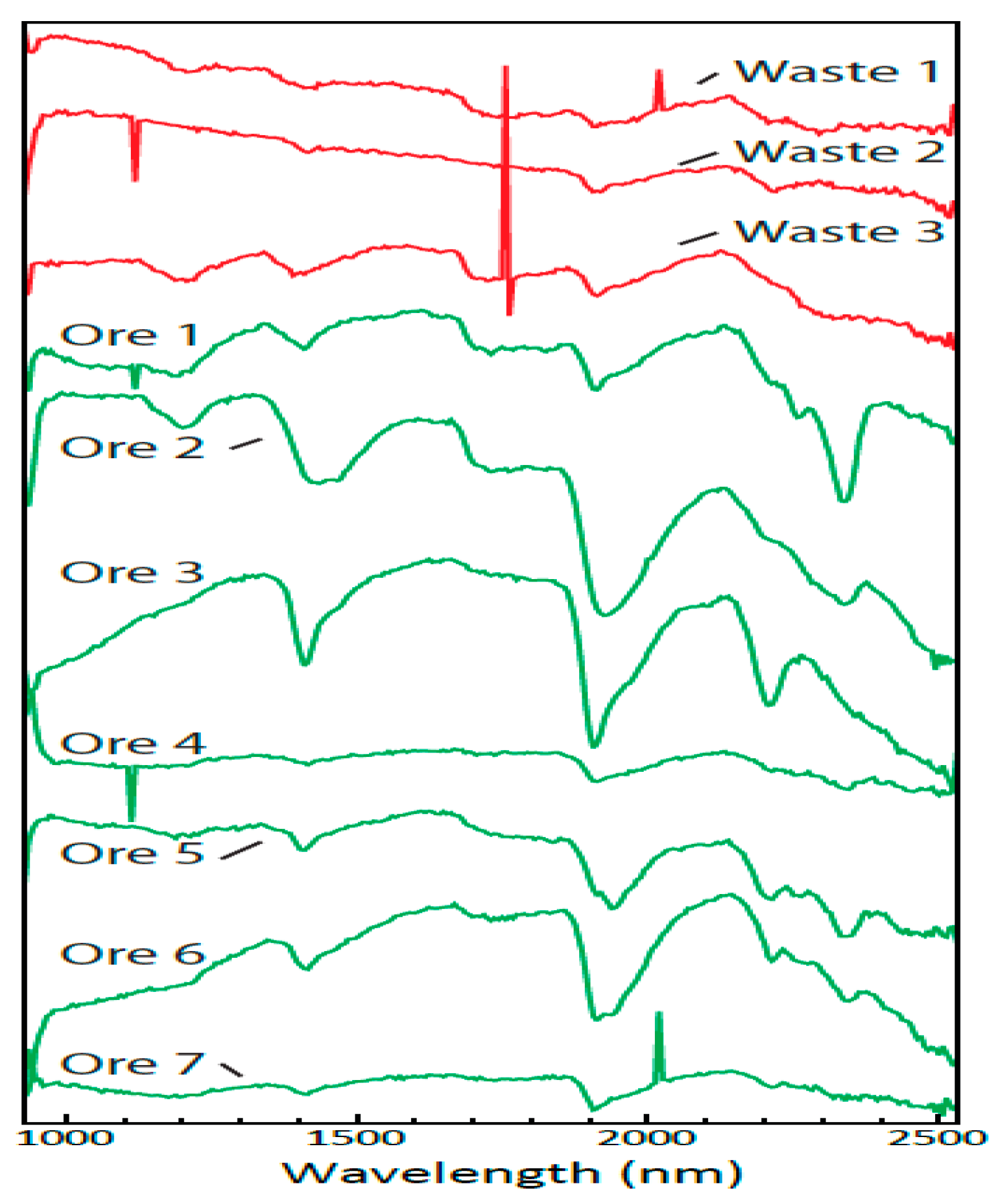
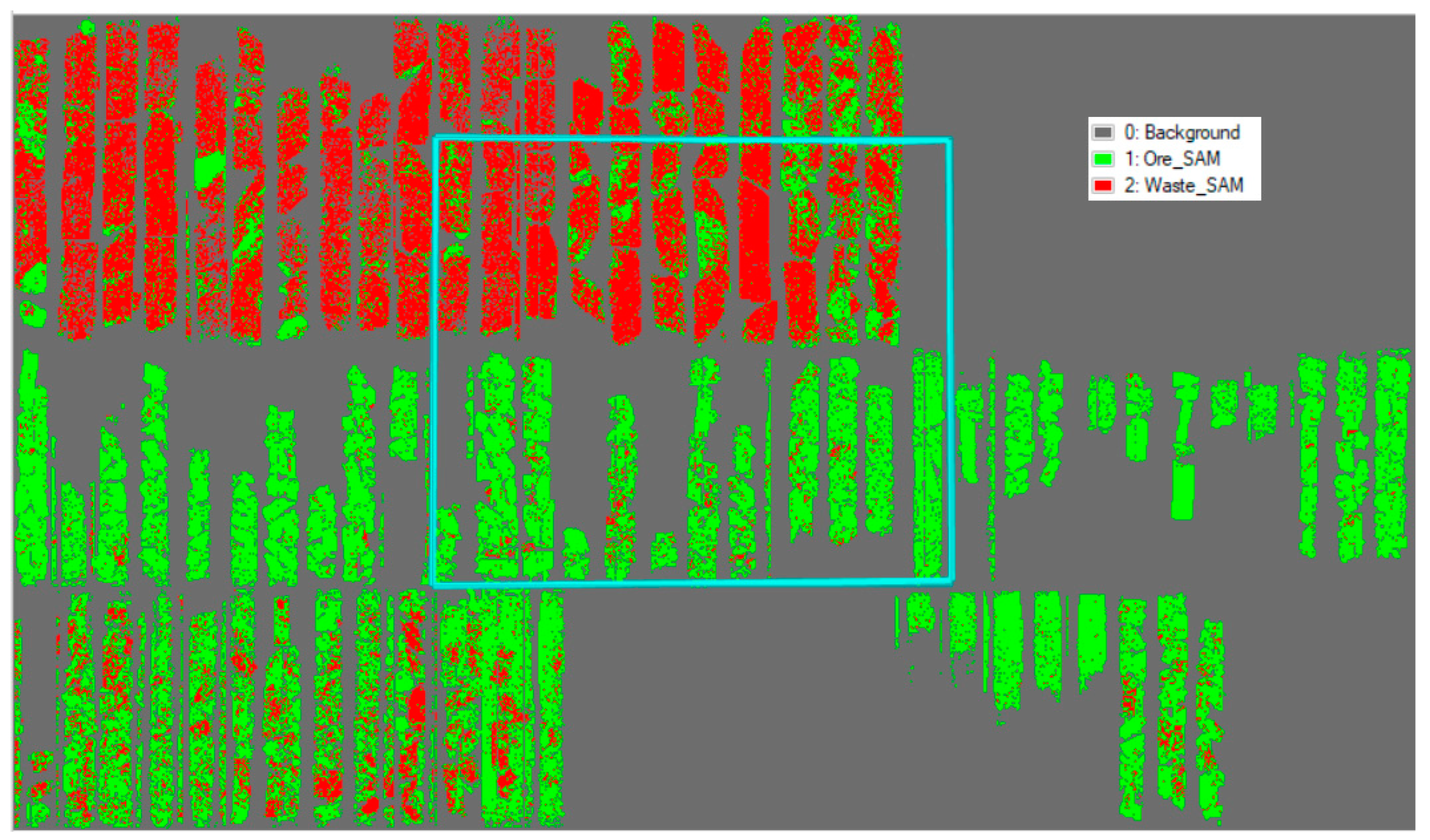
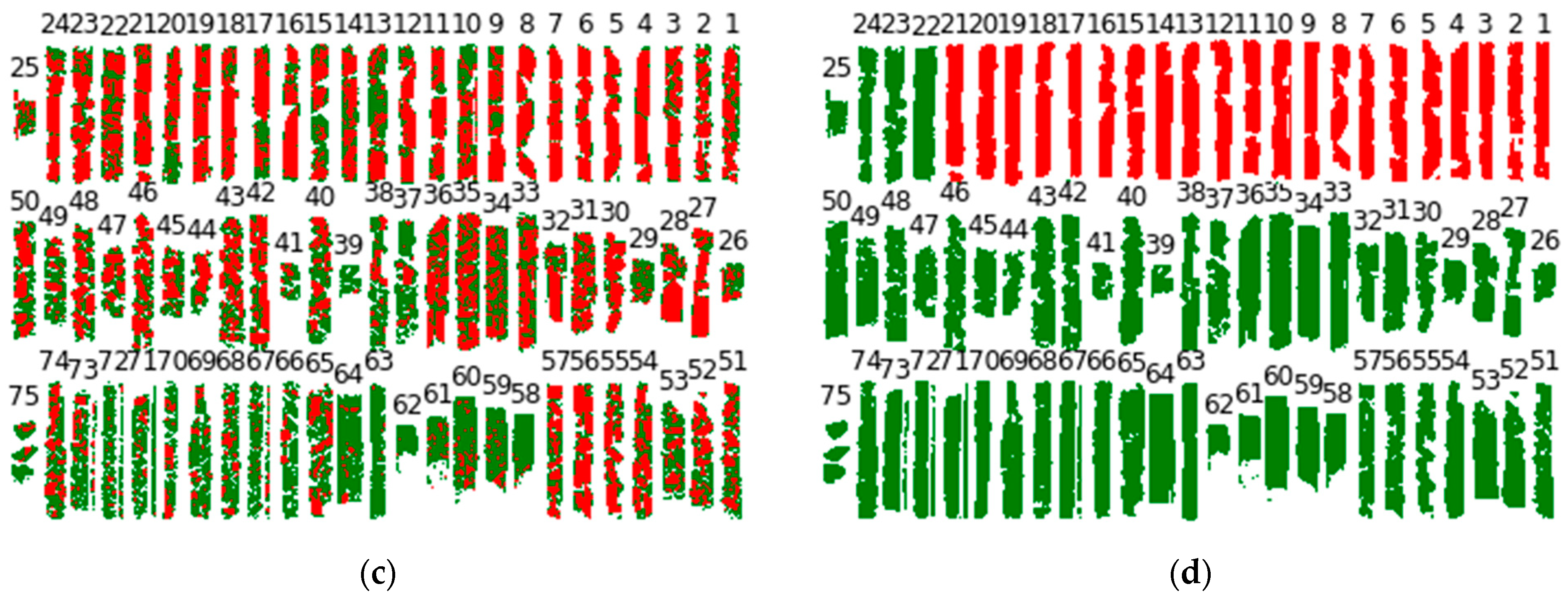
3.1. Spectral Angle Mapper Classification

As mentioned earlier, the shortwave infrared data were imported into ENVI and processed using ENVI’s spectral hourglass workflow [44]. The dimensionality of the data was reduced using a forward Minimum Noise Function (MNF) as a transformation function. This transformation reduced the full range of spectral data from 256 bands to 40. A Pixel Purity Index (PPI) was then run on the resultant MNF transformation, due to the large amount of hyperspectral data, to avoid complicated processing. The PPI allows for determining pixels that are the most spectrally unique or pure. About 30,000 iterations were run, with a threshold value of 2.5. A total of 2092 pixels were selected by the PPI. These 2092 pixels were then plotted in n-dimensional space to select spectral endmembers. Forty-one spectral endmembers were retrieved from the n-dimensional visualizer. The 41 selected endmembers were mapped across the data frame using a Spectra Angle Mapper (SAM). The SAM maximum angle was 0.10. These endmember spectra were spatially analyzed to determine their concentration in the ore or waste core boxes (Figure 1).

A sub-section of 10 spectra which were the most representative of the ore and waste fractions were selected as ore- and waste-representative spectra (Figure 4). The remaining 31 spectra were classified as background, since they did not contribute to the discrimination of ore and waste. Ore spectra have been shown in green, and waste spectra in red. In Figure 3, spectra have been vertically exaggerated by a factor of two to enhance their absorption features, and have been shown without a vertical intensity scale for ease of viewing. The seven ore spectra show several strong absorption features at approximately 1200, 1900, 2200, and 2350 nanometers. In contrast, the three waste spectra show weak absorption features at 1200, 1400, 1700, and 1900 nanometers.

Using three selected representative spectra for waste and seven representative spectra for ore as reference spectra, SAM was applied to the dataset to classify ore and waste in each pixel of the core samples. Figure 5 shows the classified image using the SAM method, where waste was labeled red, and ore was labeled green. The pixels not classified as ore or waste in the core samples were labeled as background.

3.2. Deep Learning Classification

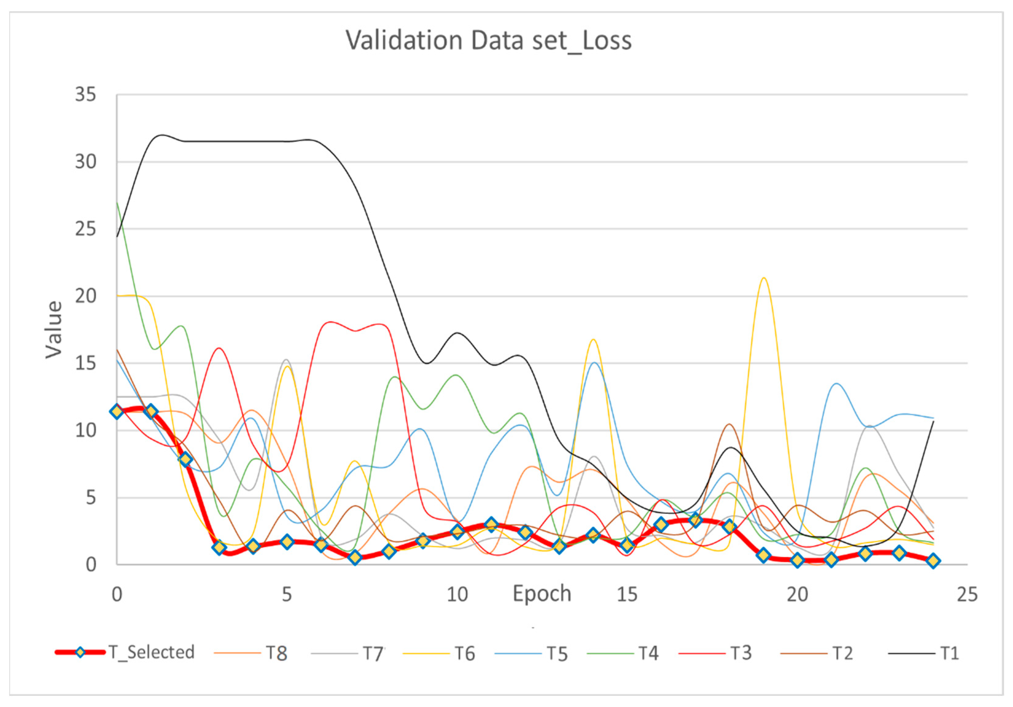
3.2.1. Model Training and Validation

Training samples in the DL model were created based on the mapped reference spectra in Figure 4 (representative spectra for waste and ore mapped using SAM). The output is a map with two classes, ore and waste. Then, pixels with high values for each class are selected as labeled pixels and used for the DL training model. Thresholding is based on the Standard Deviation (SD) method in which values above mean + 2 SD are selected as high values for each separated class. SAM was used to select accurate training data at the pixel level, to reduce the impact of the ground truth data labeled in the field.

Nalepa et al. [29] studied the validation of hyperspectral image segmentation. They concluded that conventional methods for splitting samples into training and testing sets could lead to an over-optimistic conclusion about segmentation performance, because of data leaks between the training and testing sets. To avoid this problem, and due to the large size of hyperspectral data, a subset of the hyperspectral image was used for training in this study.

Different numbers of subsets with differences in size, location, and training/validation split were used to train the model. The search area to find the best training subset was limited to the first two rows of the cores, which contain core samples from both the ore and waste boxes, and the third row is completely held out. Then, the curves for validation loss and validation F1 score were provided for some of the mentioned subsets with the same parameters at different locations delineated in Figure 6. These areas are labeled as T series (T stands for the number of the subset). A subset based on a low loss and a high F1 score was selected as the optimum subset for the final model training and classification (T-selected). This subset is indicated in Figure 1 using the blue rectangle. In this subset, there is a balance between ore and waste cores, located in the center of the image and covering around 40% of the total image. To avoid contamination (leaking data) of the whole dataset, the area beyond the selected optimum subset was held out during training of the model, and was used to test the model’s performance (around 60% of the total image).

The training time of the model was 1 h 13 min and 50 s, equal to 4430 s for the single run. The training image size is 13,198,374 pixels (3906 columns by 3379 rows) with a spatial resolution of 3 pixels/mm; each pixel contains 256 band values. All experiments with ENVI Deep Learning were performed on an Intel(R) Core (TM) i9-7920x CPU @ 2.90 GHz and with NVIDIA GeForce RTX 2080 Ti GPU and 64 GB of RAM. ENVI uses the HDF5 (h5) format to save the model and the trained weights.

Table 1. Training parameters used in the deep learning model.

Training/Validation Split	80%
Patch size	256 × 256 Pixels
Number of Epochs	25
Patches per Image	100
Class Weight	0–3
Loss Weight	0.5
Optimizer	Stochastic Gradient Descent (SGD)
Momentum Coefficient	0.99
Patch Sampling Rate	16

indicates the training parameters used in the deep learning model for this study.

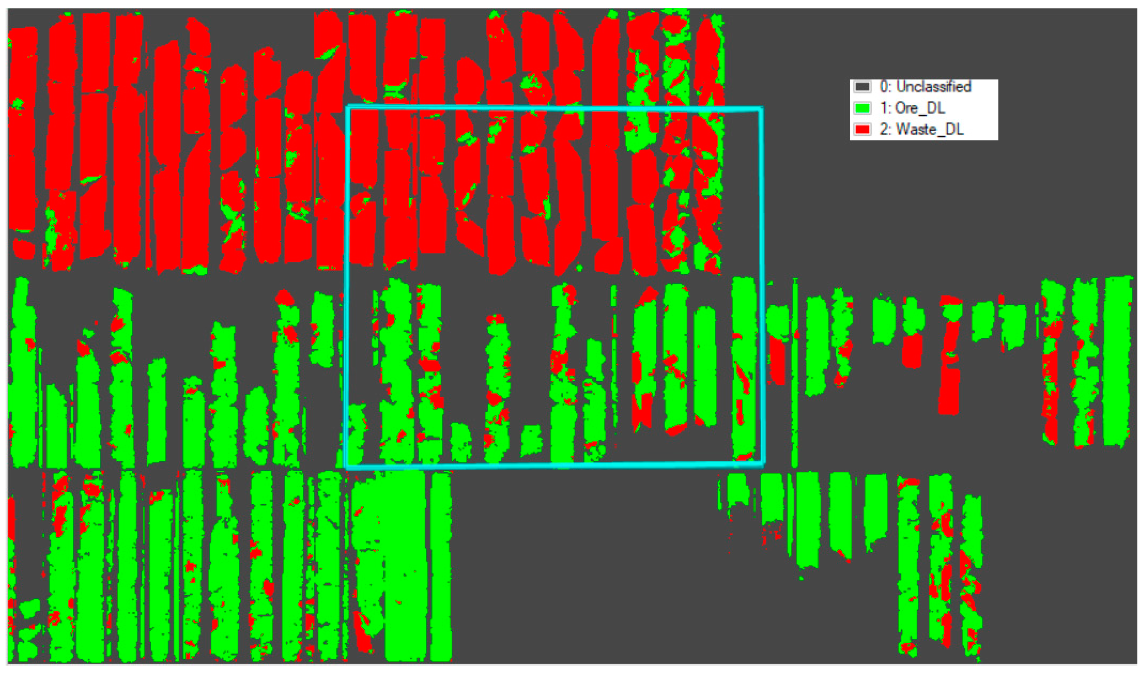
3.2.2. Image Classification

After a model learns what a specific feature looks like from the training samples, it can look for similar features in other images by classifying them. The trained model can be used to classify the whole image (Figure 1) and can also be applied to other images with a similar format and spatial and spectral properties. The end result of applying the trained model on the whole core image (training area included) was a classified raster with ore, waste, and background classes. The result of the DL classification is presented in Figure 7.

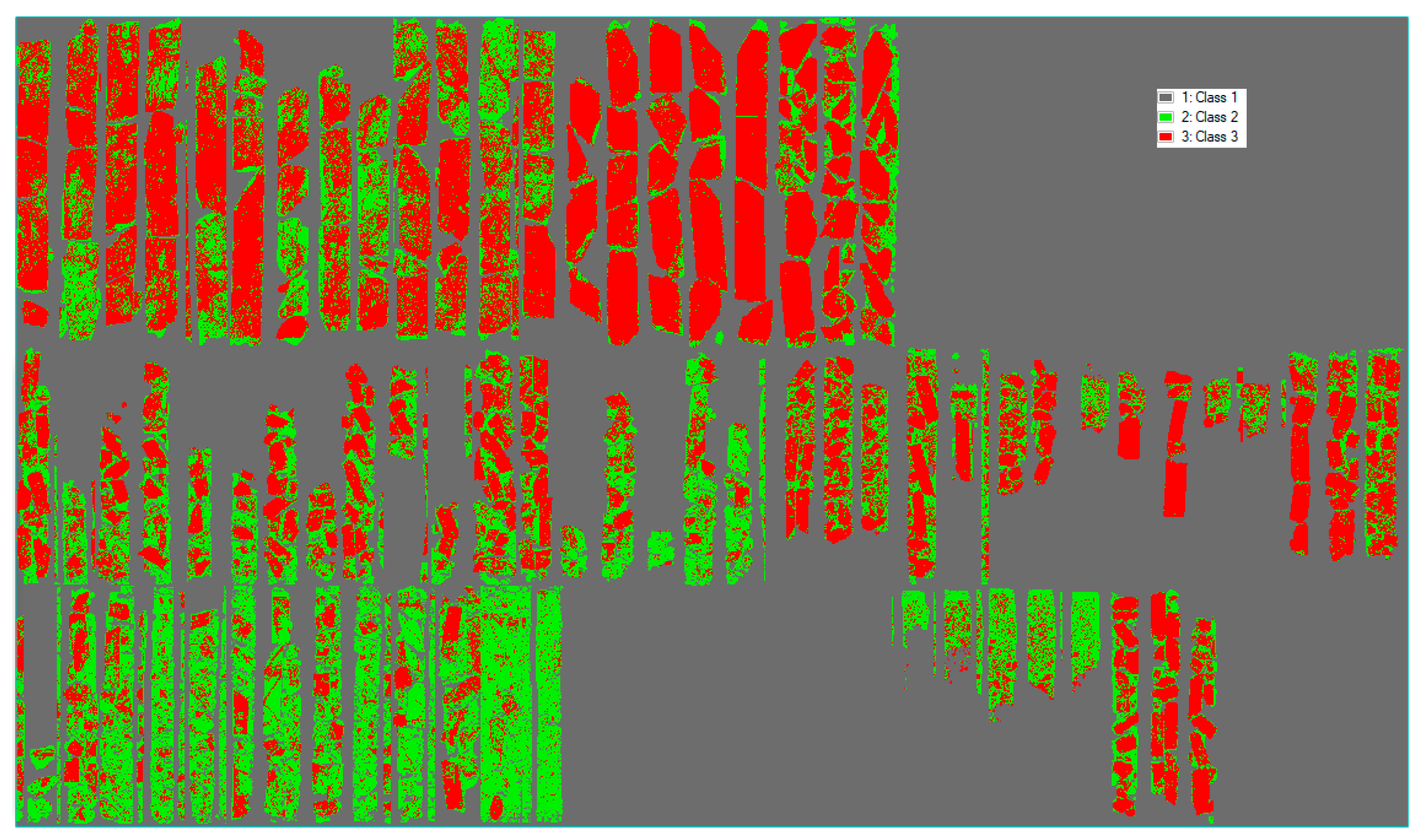
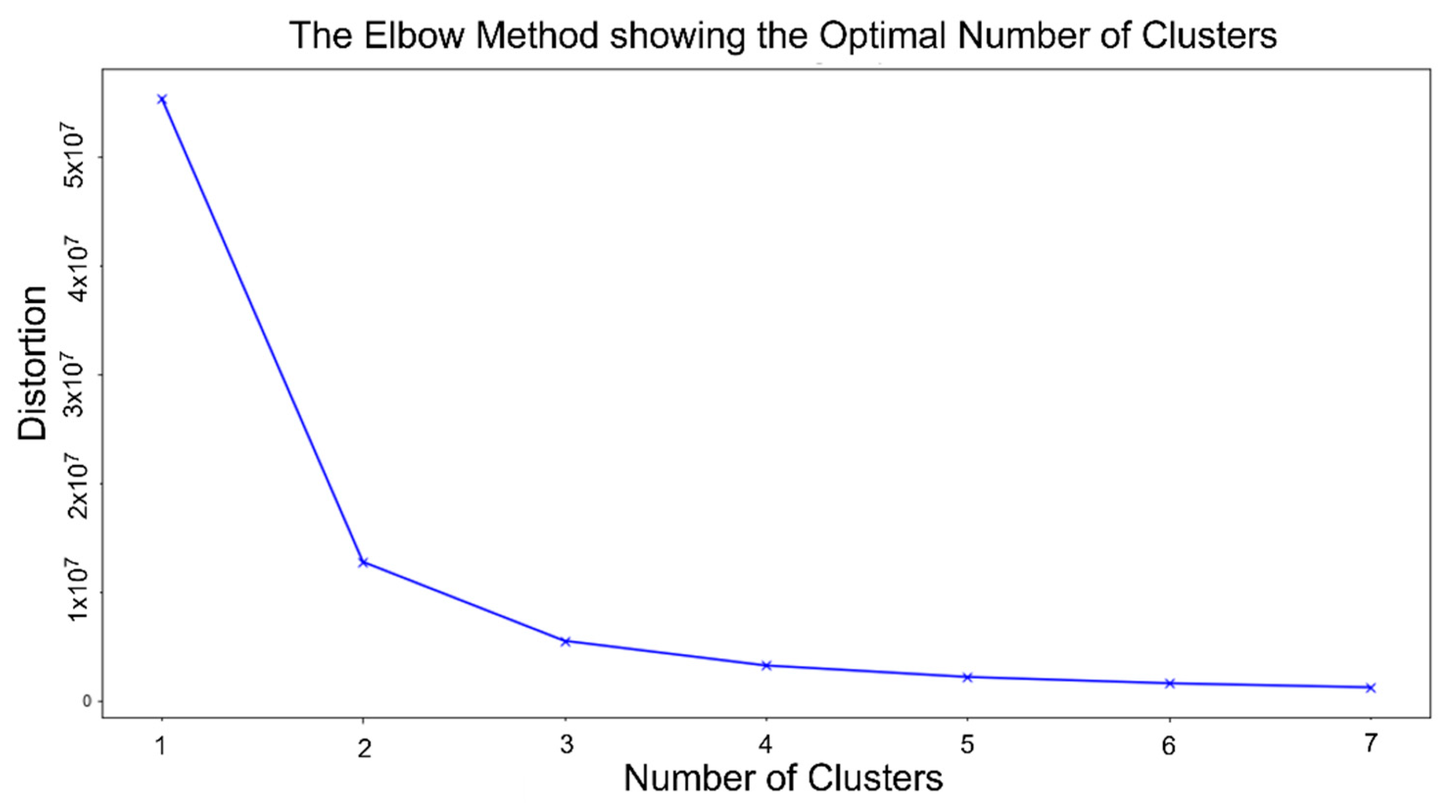
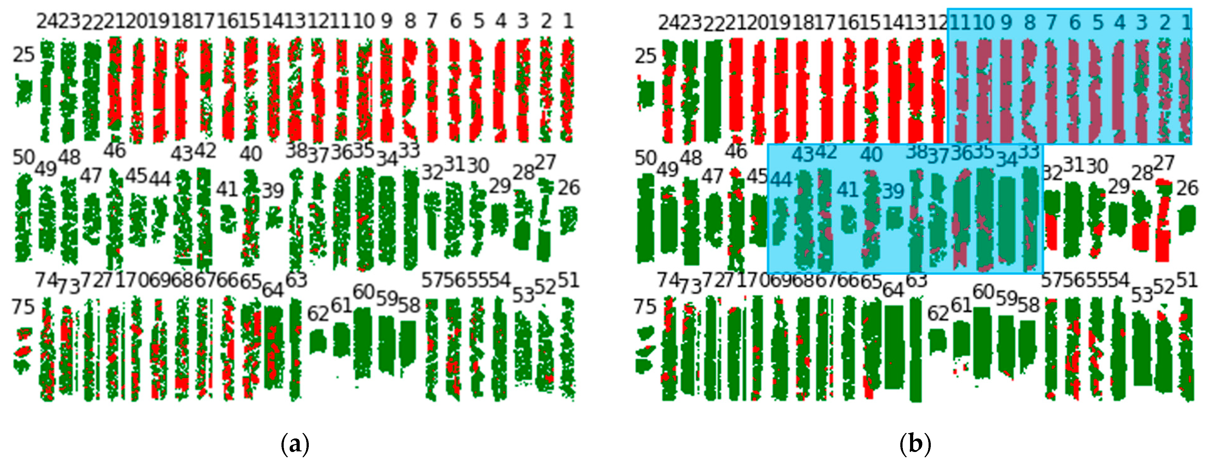
3.3. K-Means Clustering and Determining the Number of Clusters

Figure 8 illustrates the unsupervised classification using the k-means clustering technique with k = 3 and 10 iterations. One of the main classes is the image’s background, and the real number of core data classes is k − 1. So, in this classification, there are only two classes of core data which discriminate between ore and waste. The results of the unsupervised learning classification were compared with those of the SAM and DL models and verified with the ground reference image labeled based on field geologist’s reports, represented in Figure 1. The green class indicates the ore class based on its best representation in ore core boxes, and red indicates the waste class.

Figure 9 shows the output of elbow method applied to the hyperspectral dataset. From the elbow region (corresponding to k values from 2 to 4), the graph moves almost parallel to the x-axis. Based on this result, three major classes for the hyperspectral data were selected (corresponding to background, ore, and waste).

3.4. Comparing Model Performance

To compare the performance of supervised and unsupervised models (SAM, DL, and k-means) with respect to discriminating ore and waste in hyperspectral images, disagreement analysis and accuracy assessment were carried out for each separate core sample.

First, an image (that we refer to as the GT-reference image) based on ore and waste core boxes (Figure 1) was created as a reference image, representing the ground truth image. The image shows how these cores were initially labeled as ore and waste by the field geologist, based on assay analysis. Then, the classified images generated by each classifier were decomposed into 75 separate images corresponding to 75 core samples (21 waste and 54 ore samples, Figure 10). Twenty-three cores (highlighted in the blue rectangles in Figure 10b) were used for training and validation of the DL model (11 waste and 12 ore samples), and the 52 remaining cores were used to compare the performance of the models (test set), using the corresponding reference image (Figure 10d). There is a spatial consistency between the SAM- and DL-classified images. In the DL classification, nearby pixels often have the same class. That is due to an overlapping patch of pixels, as the patches of adjacent pixels will contain overlapping information [16].

Figure 11 illustrates the output image of Pixel Error (PE) disagreement analysis for each classifier, compared to the reference data (GT-reference image). The red color shows pixels which are in disagreement with the GT-reference image. The cores covered by blue rectangles (cores 1–11 and 33–44) were used in the training of the DL model, so they were removed for the purposes of model comparison. Visually it is clear that the deep learning approach generally has a better performance based on this disagreement analysis.

Table 2. Pixel Error analysis of each classifier compared with the GT-reference image on a core-by-core basis. DL: deep learning. SAM: spectral angle mapper. KM: k-means. Blue cells were removed from the models’ comparisons.

PE	25	24	23	22	21	20	19	18	17	16	15	14	13	12	(11)	(10)	(9)	(8)	(7)	(6)	(5)	(4)	(3)	(2)	(1)
DL_GT-ref	0.10	0.35	0.13	0.04	0.06	0.10	0.06	0.05	0.04	0.06	0.12	0.05	0.11	0.07	0.05	0.10	0.06	0.09	0.07	0.10	0.07	0.07	0.23	0.29	0.27
SAM_GT-ref	0.09	0.10	0.09	0.13	0.35	0.22	0.19	0.18	0.41	0.30	0.33	0.31	0.38	0.21	0.28	0.31	0.23	0.17	0.22	0.21	0.20	0.12	0.30	0.37	0.35
KM_GT-ref	0.30	0.49	0.50	0.52	0.16	0.30	0.16	0.19	0.31	0.18	0.32	0.32	0.43	0.26	0.22	0.41	0.26	0.07	0.08	0.08	0.07	0.04	0.16	0.20	0.24
	50	49	48	47	46	45	(44)	(43)	(42)	(41)	(40)	(39)	(38)	(37)	(36)	(35)	(34)	(33)	32	31	30	29	28	27	26
DL_GT-ref	0.04	0.06	0.08	0.05	0.13	0.08	0.06	0.08	0.19	0.05	0.18	0.04	0.14	0.07	0.28	0.15	0.05	0.12	0.32	0.05	0.16	0.05	0.41	0.48	0.06
SAM_GT-ref	0.16	0.13	0.10	0.10	0.13	0.13	0.13	0.16	0.14	0.09	0.21	0.15	0.20	0.18	0.15	0.17	0.16	0.11	0.12	0.13	0.09	0.12	0.11	0.07	0.12
KM_GT-ref	0.40	0.33	0.45	0.40	0.45	0.39	0.33	0.46	0.50	0.18	0.33	0.09	0.25	0.17	0.51	0.56	0.45	0.53	0.42	0.55	0.46	0.30	0.58	0.49	0.35
	75	74	73	72	71	70	69	68	67	66	65	64	63	62	61	60	59	58	57	56	55	54	53	52	51
DL_GT-ref	0.05	0.18	0.13	0.07	0.08	0.12	0.08	0.14	0.13	0.07	0.14	0.04	0.05	0.04	0.08	0.04	0.05	0.03	0.10	0.25	0.17	0.07	0.04	0.07	0.10
SAM_GT-ref	0.21	0.31	0.31	0.25	0.28	0.34	0.29	0.33	0.34	0.46	0.33	0.27	0.21	0.10	0.12	0.09	0.10	0.04	0.16	0.17	0.12	0.09	0.17	0.13	0.13
KM_GT-ref	0.13	0.37	0.27	0.20	0.23	0.34	0.23	0.33	0.25	0.26	0.38	0.21	0.15	0.09	0.21	0.26	0.23	0.14	0.43	0.55	0.45	0.48	0.35	0.42	0.34

and

Table 3. Rand Error analysis of each classifier compared with the GT-reference image on a core-by-core basis. DL: deep learning. SAM: spectral angle mapper. KM: k-means. Blue cells were removed from the models’ comparisons.

RE	25	24	23	22	21	20	19	18	17	16	15	14	13	12	(11)	(10)	(9)	(8)	(7)	(6)	(5)	(4)	(3)	(2)	(1)
DL_GT-ref	0.15	0.23	0.16	0.07	0.11	0.15	0.11	0.09	0.08	0.11	0.17	0.09	0.18	0.12	0.09	0.16	0.10	0.13	0.12	0.15	0.12	0.12	0.27	0.26	0.30
SAM_GT-ref	0.16	0.17	0.15	0.23	0.37	0.31	0.27	0.27	0.50	0.37	0.40	0.43	0.49	0.30	0.36	0.43	0.35	0.19	0.26	0.24	0.21	0.17	0.30	0.27	0.36
KM_GT-ref	0.16	0.13	0.17	0.33	0.20	0.25	0.20	0.22	0.32	0.21	0.24	0.30	0.36	0.28	0.23	0.34	0.29	0.08	0.11	0.11	0.09	0.06	0.20	0.19	0.26
	50	49	48	47	46	45	(44)	(43)	(42)	(41)	(40)	(39)	(38)	(37)	(36)	(35)	(34)	(33)	32	31	30	29	28	27	26
DL_GT-ref	0.08	0.11	0.12	0.09	0.17	0.13	0.10	0.12	0.23	0.09	0.23	0.08	0.18	0.11	0.27	0.21	0.10	0.18	0.24	0.09	0.18	0.10	0.33	0.18	0.10
SAM_GT-ref	0.27	0.22	0.18	0.18	0.22	0.21	0.22	0.26	0.22	0.14	0.30	0.24	0.29	0.27	0.22	0.27	0.26	0.20	0.21	0.22	0.16	0.22	0.19	0.12	0.20
KM_GT-ref	0.35	0.35	0.30	0.28	0.27	0.30	0.21	0.32	0.25	0.19	0.29	0.14	0.25	0.19	0.25	0.35	0.37	0.34	0.20	0.33	0.12	0.27	0.20	0.07	0.25
	75	74	73	72	71	70	69	68	67	66	65	64	63	62	61	60	59	58	57	56	55	54	53	52	51
DL_GT-ref	0.07	0.23	0.20	0.12	0.13	0.19	0.13	0.21	0.21	0.13	0.20	0.07	0.10	0.08	0.12	0.07	0.08	0.07	0.14	0.26	0.19	0.11	0.08	0.10	0.14
SAM_GT-ref	0.23	0.39	0.39	0.35	0.36	0.44	0.35	0.42	0.43	0.48	0.40	0.40	0.33	0.16	0.20	0.16	0.17	0.07	0.24	0.23	0.17	0.15	0.29	0.21	0.22
KM_GT-ref	0.13	0.35	0.32	0.27	0.30	0.41	0.27	0.38	0.34	0.35	0.37	0.32	0.24	0.10	0.20	0.29	0.24	0.16	0.26	0.21	0.18	0.30	0.40	0.28	0.24

indicate PE and RE disagreement analysis in numeric values. Blue cells indicate disagreement for cores which participated in the DL model training. These cores were removed from all three models for the purposes of performance comparison in the same condition. The minimum PE for the DL classifier with respect to waste core samples was 0.044 for core number 17, and the minimum PE for core samples was 0.035 for sample 58. In the SAM technique, the minimum PE values were 0.185 for waste core samples (core number 18) and 0.041 for ore core samples (core number 58). The lowest PE values from the k-means classification occurred in waste core sample 19 with 0.162, and in ore core number 62 with 0.090. The minimum RE values for the DL technique were 0.084 for waste core 17 and 0.0066 for ore core 58. With the SAM classifier, the minimum RE values for waste and ore cores were 0.270 and 0.074, from core numbers 19 and 58, respectively. Using the k-means technique, the minimum RE values were 0.197 and 0.069, for waste core sample 21 and ore core sample 27, respectively. In the DL and SAM techniques, the minimum PE and RE values for the ore core samples were both obtained from the same core (number 58).

Figure 12 illustrates the sorted scatter plot of the PE method to show the trend of ore and waste disagreement results separately. The x-axis indicates cores sorted based on the PE analysis values presented in Table 2. Waste and ore cores are sorted separately in red and green, but are shown in tandem in the single plot. The sorted samples belong to different core numbers and are related by different classification techniques. For example, the first core in the graph (border highlighted by blue) with the lowest PE among the waste samples for each of the three classification techniques is core number 17 for DL, 19 for k-means, and 18 for SAM. In the same way, Figure 13 shows the sorted scatter plot of the RE analysis based on Table 3.

These two plots indicate that SAM and k-means have more or less similar trends in both disagreement methods. However, the trends of the DL technique in both disagreement methods are different. In the PE_DL method, the R² value is low (0.65) due to the high amount of PE in some cores, such as core numbers 24, 28, 32, and 56 in the ore samples (Table 2).

Figure 14 shows the average disagreement analysis for total test cores (52 cores). Results indicate that based on both disagreement methods, the deep learning model performs better at discriminating between ore and waste. The best performance was by the DL method in identifying waste cores, with a PE of 0.073. k-means, an unsupervised technique, performed better than SAM, a supervised technique, for waste discrimination, in terms of having lower PE and RE values. At the same time, SAM outperformed k-means on ore discrimination based on both PE and RE values.

After creating a confusion matrix for each separate core (52 cores in total) using Python programming, a classification report was produced, including overall accuracy, precision, recall, and F1 scores for all cores in all classification techniques.

Table 4. Classification report for each technique based on the cores with maximum overall accuracy in the waste and ore groups. B: background. # indicates the core sample number. Red: waste, Green: ore.

Classification Report SAM					Classification Report k-Means					Classification Report DL
	Precision	Recall	F1-Score	Accuracy		Precision	Recall	F1-Score	Accuracy		Precision	Recall	F1-Score	Accuracy
#18 Class Waste	0.99	0.76	0.86	0.82	#19 Class Waste	0.98	0.8	0.88	0.84	#17 Class Waste	0.95	1	0.97	0.96
#58 Class Ore	0.98	0.96	0.97	0.96	#62 Class Ore	0.97	0.86	0.91	0.91	#58 Class Ore	0.95	0.99	0.97	0.97

reveals a sample of the produced classification reports for each classifier technique, using the cores with maximum overall accuracy in the waste and ore classes. Similar to the results of the disagreement analysis, k-means had a slightly better performance than SAM when identifying waste cores, with an OA of 0.84 compared to 0.82 for SAM.

Comparing classification techniques for all testing cores (52 cores) is difficult, so the weighted average of each accuracy index (weighted based on the number of pixels for each separate core) was calculated for total cores, waste cores, and ore cores. Precision for all three techniques was high, ranging above 90% (0.982, 0.975, and 0.954 for SAM, k-means, and DL, respectively). Results of the weighted averages of other indexes are presented in Figure 15, and indicate that the DL method outperformed the two other techniques. The F1 score, recall, and overall accuracy for DL are all much higher than for SAM and k-means. The precision of SAM is slightly better than that of DL and k-means, which means that the SAM method correctly identified a higher percentage of relevant results. Comparing k-means and SAM indicates that recall, F1 score, and overall accuracy with respect to the waste class are better for k-means than for SAM. So, it can be concluded, based on both the accuracy assessment matrix and disagreement analysis, that k-means performs better at waste classification than SAM.

3.5. Ensemble Image

As mentioned in the previous section, labeled images for ore and waste core boxes were created as a reference image, based on a field geologist’s interpretation of whether each box containing core samples should be labeled as ore or waste. This labeling was based solely on assay analysis for every meter of the core sample, and on the local geological information. By contrast, the labeling in the three classification methods was based on the ore and waste spectra, measured from the core samples at the pixel level (a significantly smaller scale than core level). It is recognized that there is a scale difference between the generated ground truth and the three classification methods. A core sample can contain both ore and waste spectra, but it can be classified as ore only if the grade of silver measured per meter of the core is above a cut-off grade. In order to deal with this scale difference problem, as well as to provide feedback regarding potential errors (noise) in the geologist-labelled ground truth image, a new ensemble image was created based on the results of the three classification techniques (SAM, DL, k-means). All three classification techniques were selected for creating the ensemble image because the results are generally close. SAM and k-means are the common techniques in remote sensing classification, and their results in this study are acceptable. There is a spatial consistency between the SAM- and DL-classified images. This consistency can be important in pixel labeling. In the DL classification, nearby pixels often have the same class because of an overlapping patch of pixels, but in SAM, pixels are more independent. k-means finds possible mixtures of the different classes without restriction to the reference data. In the ensemble image, we looked at the data from three different perspectives, so the output can be more accurate than the initial labeling.

In the ensemble image, for each pixel, the majority vote of ore vs. waste from the three classifiers was selected as the pixel’s label. As an example, if for one pixel two classifiers reported the pixel as ore and one as waste, this pixel was ultimately labeled as ore. Pixels with no majority vote for ore or waste were labeled as background (e.g., one technique labeled it as ore, the second technique as waste, and the last as background).

Table 5. The percentage of each core labeled as ore, waste, and background based on the voting system.

	25	24	23	22	21	20	19	18	17	16	15	14	13	12	11	10	9	8	7	6	5	4	3	2	1
Ore	0.44	0.26	0.52	0.72	0.03	0.05	0.02	0.01	0.01	0.03	0.08	0.02	0.08	0.03	0.02	0.04	0.02	0.04	0.03	0.05	0.03	0.01	0.16	0.23	0.21
Waste	0.03	0.30	0.09	0.01	0.64	0.51	0.67	0.65	0.57	0.61	0.44	0.55	0.53	0.64	0.59	0.55	0.65	0.52	0.62	0.62	0.56	0.70	0.52	0.38	0.49
Background	0.53	0.44	0.39	0.26	0.33	0.43	0.31	0.34	0.42	0.36	0.49	0.43	0.39	0.33	0.39	0.41	0.33	0.44	0.34	0.32	0.41	0.29	0.31	0.39	0.29
	50	49	48	47	46	45	44	43	42	41	40	39	38	37	36	35	34	33	32	31	30	29	28	27	26
Ore	0.67	0.63	0.63	0.65	0.56	0.62	0.52	0.65	0.55	0.57	0.51	0.59	0.52	0.56	0.42	0.65	0.75	0.70	0.31	0.77	0.42	0.68	0.34	0.09	0.63
Waste	0.01	0.02	0.03	0.01	0.11	0.05	0.02	0.06	0.14	0.01	0.14	0.00	0.09	0.03	0.24	0.12	0.03	0.09	0.25	0.00	0.12	0.00	0.34	0.43	0.00
Background	0.32	0.34	0.33	0.34	0.33	0.33	0.46	0.29	0.31	0.42	0.35	0.41	0.39	0.40	0.33	0.23	0.22	0.21	0.44	0.23	0.46	0.32	0.32	0.48	0.37
	75	74	73	72	71	70	69	68	67	66	65	64	63	62	61	60	59	58	57	56	55	54	53	52	51
Ore	0.46	0.55	0.54	0.61	0.60	0.58	0.60	0.60	0.57	0.66	0.58	0.85	0.74	0.51	0.52	0.73	0.68	0.67	0.58	0.45	0.43	0.67	0.73	0.56	0.54
Waste	0.03	0.17	0.08	0.01	0.03	0.06	0.05	0.10	0.05	0.02	0.13	0.03	0.00	0.00	0.02	0.00	0.01	0.00	0.08	0.24	0.16	0.04	0.00	0.04	0.06
Background	0.51	0.29	0.38	0.37	0.37	0.35	0.35	0.30	0.38	0.33	0.29	0.13	0.25	0.49	0.46	0.26	0.31	0.33	0.34	0.31	0.42	0.29	0.26	0.40	0.40

displays the percentage of each core labeled as ore, waste, and background, after applying the voting system to generate the new ensemble image (depicted in Figure 16).

4. Discussion

Deep learning, a relatively new research area in hyperspectral image classification, offers great potential for ore and waste discrimination. This research is one of the first attempts to use ENVI deep learning modules to discriminate ore and waste based on hyperspectral data collected from core samples. The results show that the DL method trained on labels generated by SAM has a better performance, based on disagreement analysis and accuracy assessment, than the two other classifiers (SAM and k-means). The model input for the DL model is the label raster that can automatically generate semantic features to identify classes. The training of the deep learning model involves some random process due to how this algorithm attempts to converge [34,43]. This random splitting between test and training data leads to over-optimistic segmentation performance [29]. To avoid data contamination in the comparison process, the cores that participated in the training of the DL model were removed.

In the DL training model, the value of training loss rapidly decreases in the first few epochs and continues decreasing until the end epoch (Figure 5). The minimum validation loss happened on the last epoch, so the model did not lose the ability to generalize predictions for the test datasets during the training.

In this study, the overall accuracy, F1 score, and recall of ore and waste discrimination using DL were high compared to SAM and k-means. However, the precision was slightly lower than SAM and k-means (around 0.03 difference). This means that in addition to increasing the true positives, there were more false positives in the DL method than in the SAM and k-means techniques. This can be attributed to the fact that in the DL classification, nearby pixels often have the same class, so the patches of adjacent pixels will contain overlapping information.

The trend of RE (Figure 12) indicates that the three classification techniques are similar in topological view with respect to classifing pixels or detecting object boundaries in the image, particularly for the ore cores. RE disagreement focuses on class boundaries and evaluates structures’ completeness for nearby pixels belonging to the same class. The RE increases slightly when there are minor differences in the location of class boundaries, but a large amount of RE occurs by merging or splitting pixel classes. The average amount of RE for all models (Figure 14) indicates a significant difference for the SAM technique, which has a high RE, particularly in waste core samples, compared to the two other models, and signifies the poor performance of SAM in the discrimination of waste samples. Contrary to RE, PE evaluates the classification performance pixel by pixel, and the result is not affected by nearby pixels. The PE trend (Figure 11) signifies that SAM and DL are similar with respect to ore cores, but that SAM and k-means are very close regarding waste cores. Overall, based on PE, k-means is far from the other two classification techniques for identifying ore cores and has poor performance in this regard.

Figure 14 and Figure 15 show that k-means performs better than SAM for waste cores, based on disagreement analysis and accuracy assessment. These results indicate that k-means, as an unsupervised technique, can produce a simple classification of ore and waste based on hyperspectral data.

The initial ground truth reference model (GT-reference image) was generated for each core box based on the field geology interpretation. However, due to a mixture of both ore and waste spectra measured in each core sample, the ore/waste classification based on hyperspectral imaging occurs at the pixel-by-pixel scale. Given this scale discrepancy, a new ensemble image was created based on a voting system incorporating the (generally close) results from the three classifiers. The new ensemble image can be used to identify core samples with high disagreements (i.e., samples #2, #27, #28, #56) as samples with potential noise (prompting further testing to ascertain that they have been well classified as either ore or waste based on the geological interpretation).

5. Conclusions

Ore and waste discrimination is an essential step in mining operations. Hyperspectral imaging is an effective method for discriminating between ore and waste. In this study, hyperspectral analysis of core samples was used to compare the performance of the ENVI deep learning module against the Spectral Angle Mapper and k-means techniques, well-known supervised and unsupervised machine learning methods for ore/waste discrimination. Disagreement analysis, namely Rand Error and Pixel Error, as well as accuracy assessment indices, including loss, accuracy, precision, recall, and F1 score, were used to evaluate the performance of the three classifier methods. The results demonstrated that the DL method outperformed the other two techniques. The overall accuracy of the DL model was 0.89, the F1 score was 0.91, the recall was 0.89, and the precision was 0.95, which indicates good agreement in the discrimination of the ore and waste dataset. A comparison with the k-means and SAM classification techniques showed that in the waste part of the dataset, k-means classification had better performance than SAM. The Rand Error for SAM in the waste part is high, indicating that from a topological view, there are big differences between the boundaries of predicted classes and those of the reference image.

When using the DL technique, the initial classification and class activation rasters may not be entirely accurate, depending on the quality of the input training samples. An optional step would be to refine the label rasters by creating regions of interest (ROIs) of the highest pixel values, then editing the ROIs to remove false positives. The refined ROIs can be combined with the original ROIs to train a new model or refine the trained model and improve classification results. In general, the results presented showed that the ENVI deep learning techniques can effectively discriminate ore and waste in a near real-time manner.

The evaluation of the models in this study was based on available information, with a focus on only ore/waste discrimination in the core samples, and the results in the scope of the research are acceptable. The core samples were scanned in a laboratory under ideal lighting conditions. The illumination conditions in the field might cause major issues in the acquisition and analysis of hyperspectral data. No attempt was made to use the hyperspectral data to classify the ore samples based on their grade. This is an ongoing study, and these additional challenges will be addressed in future work.

References

1. Benndorf, J.; Buxton, M.W.N. Sensor-Based Real-Time Resource Model Reconciliation for Improved Mine Production Control—A Conceptual Framework. Min. Technol. 2016, 125, 54–64. [Google Scholar] [CrossRef] [Green Version]
2. Christoffersen, P.; Esmaeili, K.; Rivard, B.; Feng, J.; Osinski, G. Developing Spectral Ore-Waste Discrimination Methods: A Case Study at the El Gallo Silver Deposit, Mexico. In Proceedings of the AME Roundup, Vancouver, BC, Canada, 20–23 January 2020. [Google Scholar]
3. Ohadi, B.; Esmaeili, K. Statistical Analysis of Blast-Induced Rock Movement- A Case Study at Detour Lake Mine. In Proceedings of the CIM Conference, Montreal, QC, Canada, 30 April–3 May 2017. [Google Scholar]
4. van der Meer, F.D.; van der Werff, H.M.A.; van Ruitenbeek, F.J.A.; Hecker, C.A.; Bakker, W.H.; Noomen, M.F.; van der Meijde, M.; Carranza, E.J.M.; de Smeth, J.B.; Woldai, T. Multi- and Hyperspectral Geologic Remote Sensing: A Review. Int. J. Appl. Earth Obs. Geoinf. 2012, 14, 112–128. [Google Scholar] [CrossRef]
5. Samanta, B.; Manna, B.; Chakravarty, D.; Dutta, D. Assessment of Hyperspectral Sampling Based Analysis Technique for Copper Grade Estimation at a Concentrator Plant. J. Powder Metall. Min. 2017, 6, 184. [Google Scholar] [CrossRef]
6. Abdolmaleki, M.; Fathianpour, N.; Tabaei, M. Evaluating the Performance of the Wavelet Transform in Extracting Spectral Alteration Features from Hyperspectral Images. Int. J. Remote Sens. 2018, 39, 6076–6094. [Google Scholar] [CrossRef]
7. Wills, B.A.; Finch, J.A. Sensor-Based Ore Sorting. In Wills’ Mineral Processing Technology; Elsevier: Amsterdam, The Netherlands, 2016; pp. 409–416. [Google Scholar]
8. Buxton, M.W.N.; Benndorf, J. The Use of Sensor Derived Data in Optimization along the Mine-Value-Chain. In Proceedings of the 15th international ISM Congress, Aachen, Germany, 16–20 September 2013; pp. 324–336. [Google Scholar]
9. Dalm, M.; Buxton, M.W.N.; van Ruitenbeek, F.J.A. Ore–Waste Discrimination in Epithermal Deposits Using Near-Infrared to Short-Wavelength Infrared (NIR-SWIR) Hyperspectral Imagery. Math. Geosci. 2019, 51, 849–875. [Google Scholar] [CrossRef] [Green Version]
10. Bamford, T.; Esmaeili, K.; Schoellig, A.P. A Deep Learning Approach for Rock Fragmentation Analysis. Int. J. Rock Mech. Min. Sci. 2021, 145, 104839. [Google Scholar] [CrossRef]
11. Tang, M.; Esmaeili, K. Heap Leach Pad Surface Moisture Monitoring Using Drone-Based Aerial Images and Convolutional Neural Networks: A Case Study at the El Gallo Mine, Mexico. Remote Sens. 2021, 13, 1420. [Google Scholar] [CrossRef]
12. Ohadi, B.; Sun, X.; Esmaieli, K.; Consens, M.P. Predicting Blast-Induced Outcomes Using Random Forest Models of Multi-Year Blasting Data from an Open Pit Mine. Bull. Eng. Geol. Environ. 2020, 79, 329–343. [Google Scholar] [CrossRef]
13. Cracknell, M.J.; Reading, A.M. Geological Mapping Using Remote Sensing Data: A Comparison of Five Machine Learning Algorithms, Their Response to Variations in the Spatial Distribution of Training Data and the Use of Explicit Spatial Information. Comput. Geosci. 2014, 63, 22–33. [Google Scholar] [CrossRef] [Green Version]
14. Beretta, F.; Rodrigues, A.L.; Peroni, R.L.; Costa, J.F.C.L. Automated Lithological Classification Using UAV and Machine Learning on an Open Cast Mine. Appl. Earth Sci. 2019, 128, 79–88. [Google Scholar] [CrossRef]
15. Barton, I.F.; Gabriel, M.J.; Lyons-Baral, J.; Barton, M.D.; Duplessis, L.; Roberts, C. Extending Geometallurgy to the Mine Scale with Hyperspectral Imaging: A Pilot Study Using Drone- and Ground-Based Scanning. Min. Met. Explor. 2021, 38, 799–818. [Google Scholar] [CrossRef]
16. Choros, K.A.; Job, A.T.; Edgar, M.L.; Austin, K.J.; McAree, P.R. Can Hyperspectral Imaging and Neural Network Classification Be Used for Ore Grade Discrimination at the Point of Excavation? Sensors 2022, 22, 2687. [Google Scholar] [CrossRef] [PubMed]
17. Sinaice, B.B.; Owada, N.; Ikeda, H.; Toriya, H.; Bagai, Z.; Shemang, E.; Adachi, T.; Kawamura, Y. Spectral Angle Mapping and AI Methods Applied in Automatic Identification of Placer Deposit Magnetite Using Multispectral Camera Mounted on UAV. Minerals 2022, 12, 268. [Google Scholar] [CrossRef]
18. Petropoulos, G.P.; Vadrevu, K.P.; Xanthopoulos, G.; Karantounias, G.; Scholze, M. A Comparison of Spectral Angle Mapper and Artificial Neural Network Classifiers Combined with Landsat TM Imagery Analysis for Obtaining Burnt Area Mapping. Sensors 2010, 10, 1967–1985. [Google Scholar] [CrossRef] [PubMed] [Green Version]
19. Liu, Y.; Zhang, Z.; Liu, X.; Wang, L.; Xia, X. Ore Image Classification Based on Small Deep Learning Model: Evaluation and Optimization of Model Depth, Model Structure and Data Size. Min. Eng. 2021, 172, 107020. [Google Scholar] [CrossRef]
20. Minaee, S.; Boykov, Y.Y.; Porikli, F.; Plaza, A.J.; Kehtarnavaz, N.; Terzopoulos, D. Image Segmentation Using Deep Learning: A Survey. IEEE Trans. Pattern Anal. Mach. Intell. 2021, 44, 3523–3542. [Google Scholar] [CrossRef]
21. Chen, Z.; Liu, X.; Yang, J.; Little, E.; Zhou, Y. Deep Learning-Based Method for SEM Image Segmentation in Mineral Characterization, an Example from Duvernay Shale Samples in Western Canada Sedimentary Basin. Comput. Geosci. 2020, 138, 104450. [Google Scholar] [CrossRef]
22. Roy, A.G.; Navab, N.; Wachinger, C. Concurrent Spatial and Channel ’Squeeze & Excitation’ in Fully Convolutional Networks. In Proceedings of the International Conference on Medical Image Computing and Computer-Assisted Intervention, Granada, Spain, 16–20 September 2018; Springer International Publishing: Cham, Germany, 2018; pp. 421–429. [Google Scholar]
23. Desta, F.; Buxton, M. Image and Point Data Fusion for Enhanced Discrimination of Ore and Waste in Mining. Minerals 2020, 10, 1110. [Google Scholar] [CrossRef]
24. MacQueen, J.B. Some Methods for Classification and Analysis of Multivariate Observations. In Proceedings of the 5th Berkeley Symposium on Mathematical Statistics and Probability; Le Cam, L.M., Neyman, J., Eds.; University of California Press: Berkeley, CA, USA, 1967; pp. 281–297. [Google Scholar]
25. Paoletti, M.E.; Haut, J.M.; Plaza, J.; Plaza, A. Deep Learning Classifiers for Hyperspectral Imaging: A Review. ISPRS J. Photogramm. Remote Sens. 2019, 158, 279–317. [Google Scholar] [CrossRef]
26. Rangnekar, A.; Mokashi, N.; Ientilucci, E.J.; Kanan, C.; Hoffman, M.J. AeroRIT: A New Scene for Hyperspectral Image Analysis. IEEE Trans. Geosci. Remote Sens. 2020, 58, 8116–8124. [Google Scholar] [CrossRef]
27. Okada, N.; Maekawa, Y.; Owada, N.; Haga, K.; Shibayama, A.; Kawamura, Y. Automated Identification of Mineral Types and Grain Size Using Hyperspectral Imaging and Deep Learning for Mineral Processing. Minerals 2020, 10, 809. [Google Scholar] [CrossRef]
28. Lypaczewski, P.; Rivard, B.; Gaillard, N.; Perrouty, S.; Piette-Lauzière, N.; Bérubé, C.L.; Linnen, R.L. Using Hyperspectral Imaging to Vector towards Mineralization at the Canadian Malartic Gold Deposit, Québec, Canada. Ore Geol. Rev. 2019, 111, 102945. [Google Scholar] [CrossRef]
29. Nalepa, J.; Myller, M.; Kawulok, M. Validating Hyperspectral Image Segmentation. IEEE Geosci. Remote Sens. Lett. 2019, 16, 1264–1268. [Google Scholar] [CrossRef] [Green Version]
30. Abdolmaleki, M.; Tabaei, M.; Fathianpour, N.; Gorte, B.G.H. Selecting Optimum Base Wavelet for Extracting Spectral Alteration Features Associated with Porphyry Copper Mineralization Using Hyperspectral Images. Int. J. Appl. Earth Obs. Geoinf. 2017, 58, 134–144. [Google Scholar] [CrossRef]
31. Lorenz, S.; Salehi, S.; Kirsch, M.; Zimmermann, R.; Unger, G.; Vest Sørensen, E.; Gloaguen, R. Radiometric Correction and 3D Integration of Long-Range Ground-Based Hyperspectral Imagery for Mineral Exploration of Vertical Outcrops. Remote Sens. 2018, 10, 176. [Google Scholar] [CrossRef] [Green Version]
32. Kurz, T.H.; Buckley, S.J.; Howell, J.A. Close-Range Hyperspectral Imaging for Geological Field Studies: Workflow and Methods. Int. J. Remote Sens. 2013, 34, 1798–1822. [Google Scholar] [CrossRef]
33. Kruse, F.A.; Lefkoff, A.B.; Boardman, J.W.; Heidebrecht, K.B.; Shapiro, A.T.; Barloon, P.J.; Goetz, A.F.H. The Spectral Image Processing System (SIPS)—Interactive Visualization and Analysis of Imaging Spectrometer Data. Remote Sens. Environ. 1993, 44, 145–163. [Google Scholar] [CrossRef]
34. Fetai, B.; Račič, M.; Lisec, A. Deep Learning for Detection of Visible Land Boundaries from UAV Imagery. Remote Sens. 2021, 13, 2077. [Google Scholar] [CrossRef]
35. Ronneberger, O.; Fischer, P.; Brox, T. U-Net: Convolutional Networks for Biomedical Image Segmentation. In; Springer International Publishing: Cham, Switzerland, 2015; pp. 234–241. [Google Scholar]
36. L3 Harris Geospatial Pixel Segmentation Training Background. Available online: https://www.l3harrisgeospatial.com/docs/PixelSegmentationTrainingBackground.html (accessed on 9 May 2022).
37. Sood, V.; Tiwari, R.K.; Singh, S.; Kaur, R.; Parida, B.R. Glacier Boundary Mapping Using Deep Learning Classification over Bara Shigri Glacier in Western Himalayas. Sustainability 2022, 14, 13485. [Google Scholar] [CrossRef]
38. Lv, Z.; Hu, Y.; Zhong, H.; Wu, J.; Li, B.; Zhao, H. Parallel K-Means Clustering of Remote Sensing Images Based on MapReduce. In Proceedings of the International Conference on Web Information Systems and Mining, Sanya, China, 23–24 October 2010; pp. 162–170. [Google Scholar]
39. Liu, L.; Peng, Z.; Wu, H.; Jiao, H.; Yu, Y.; Zhao, J. Fast Identification of Urban Sprawl Based on K-Means Clustering with Population Density and Local Spatial Entropy. Sustainability 2018, 10, 2683. [Google Scholar] [CrossRef]
40. Umargono, E.; Suseno, J.E.; Vincensius Gunawan, S.K. K-Means Clustering Optimization Using the Elbow Method and Early Centroid Determination Based-on Mean and Median. In Proceedings of the International Conferences on Information System and Technology, Cairo, Egypt, 24–26 March 2019; SCITEPRESS—Science and Technology Publications: Setubal, Portugal, 2019; pp. 234–240. [Google Scholar]
41. Zhu, F.; Liu, Q.; Fu, Y.; Shen, B. Segmentation of Neuronal Structures Using SARSA (λ)-Based Boundary Amendment with Reinforced Gradient-Descent Curve Shape Fitting. PLoS ONE 2014, 9, e90873. [Google Scholar] [CrossRef] [PubMed]
42. Liu, L.-Y.; Wang, C.-K. BUILDING SEGMENTATION IN AGRICULTURAL LAND USING HIGH RESOLUTION SATELLITE IMAGERY BASED ON DEEP LEARNING APPROACH. Int. Arch. Photogramm. Remote Sens. Spat. Inf. Sci. 2021, XLIII-B3-2021, 587–594. [Google Scholar] [CrossRef]
43. Zhang, P.; Xu, C.; Ma, S.; Shao, X.; Tian, Y.; Wen, B. Automatic Extraction of Seismic Landslides in Large Areas with Complex Environments Based on Deep Learning: An Example of the 2018 Iburi Earthquake, Japan. Remote Sens. 2020, 12, 3992. [Google Scholar] [CrossRef]
44. Wolfe, J.D.; Black, S.R. Hyperspectral Analytics in ENVI Target. Detection and Spectral Mapping Methods; Harris Corporation: Melbourne, FL, USA, 2018. [Google Scholar]
Figure 1. Hyperspectral near-infrared image of scanned drill core samples. The blue rectangle indicates the training area for deep learning analysis.
Remotesensing 14 06386 g001
Figure 2. Workflow for ore and waste classification based on SAM, the ENVINet5 model, and k-means clustering.
Remotesensing 14 06386 g002
Figure 3. Diagram of the ENVI-Net architecture which presents how the model processes a single patch. Modified parts highlighted by red rectangles (modified from [36]).
Remotesensing 14 06386 g003
Figure 4. Spectral plot showing the 10 ore and waste spectra selected from the 41 endmembers classified from the n-dimensional visualization step. Ore: green, Waste: red.
Remotesensing 14 06386 g004
Figure 5. Classified image showing spectral classes identified by the SAM. Ore is shown in green, and waste is shown in red. Blue rectangle: training area for DL analysis.
Remotesensing 14 06386 g005
Figure 6. Line chart of the loss and F1 score in the validation dataset for different subsets (red line with yellow diamond dots indicates the selected subset). T: tested subset used for selecting optimum training area.
Remotesensing 14 06386 g006aRemotesensing 14 06386 g006b
Figure 7. Classified image showing ore and waste classes identified by ENVI deep learning. (Red: waste, Green: ore, Blue rectangle: training area).
Remotesensing 14 06386 g007
Figure 8. k-means clustering (with k = 3) applied to the hyperspectral dataset. (Red: waste, Green: ore).
Remotesensing 14 06386 g008
Figure 9. The elbow method for determining the number of clusters.
Remotesensing 14 06386 g009
Figure 10. Core sample images were labeled by different classifiers (23 cores for training and validation highlighted in blue rectangles, 52 cores for testing). (a): SAM classification; (b): deep learning classification; (c): k-means classification; (d): GT-reference image. Red: waste, Green: ore.
Remotesensing 14 06386 g010aRemotesensing 14 06386 g010b
Figure 11. Pixel error disagreement analysis (23 cores used for training, highlighted in blue rectangles, and 52 cores for testing). (a): SAM vs. GT-reference; (b): deep learning vs. GT-reference; (c): k-means vs. GT-reference. Red: pixels with disagreement, Blue rectangles: cores removed from disagreement analysis comparison.
Remotesensing 14 06386 g011
Figure 12. Pixel Error disagreement analysis. D: deep learning. S: SAM. K: k-means. Red: Waste. Green: Ore. The x-axis indicates cores sorted based on PE analysis values presented in Table 2.
Remotesensing 14 06386 g012
Figure 13. Rand Error disagreement analysis. D: deep learning. S: SAM. K: k-means. Red: Waste. Green: Ore. The x-axis indicates cores sorted based on RE analysis values presented in Table 3.
Remotesensing 14 06386 g013
Figure 14. The averages of PE and RE analyses for all cores without training data. AVE: the average value of disagreement analysis.
Remotesensing 14 06386 g014
Figure 15. The weighted averages of classification reports for each technique (applied to 52 cores).
Remotesensing 14 06386 g015
Figure 16. New ensemble image based on the voting system. Red: Waste, Green: Ore.
Remotesensing 14 06386 g016