
Evaluation of Hybrid Wavelet Models for Regional Drought Forecasting
 , ,
, ,  and
and
Abstract
:
1. Introduction
2. Study Area and Data Collection
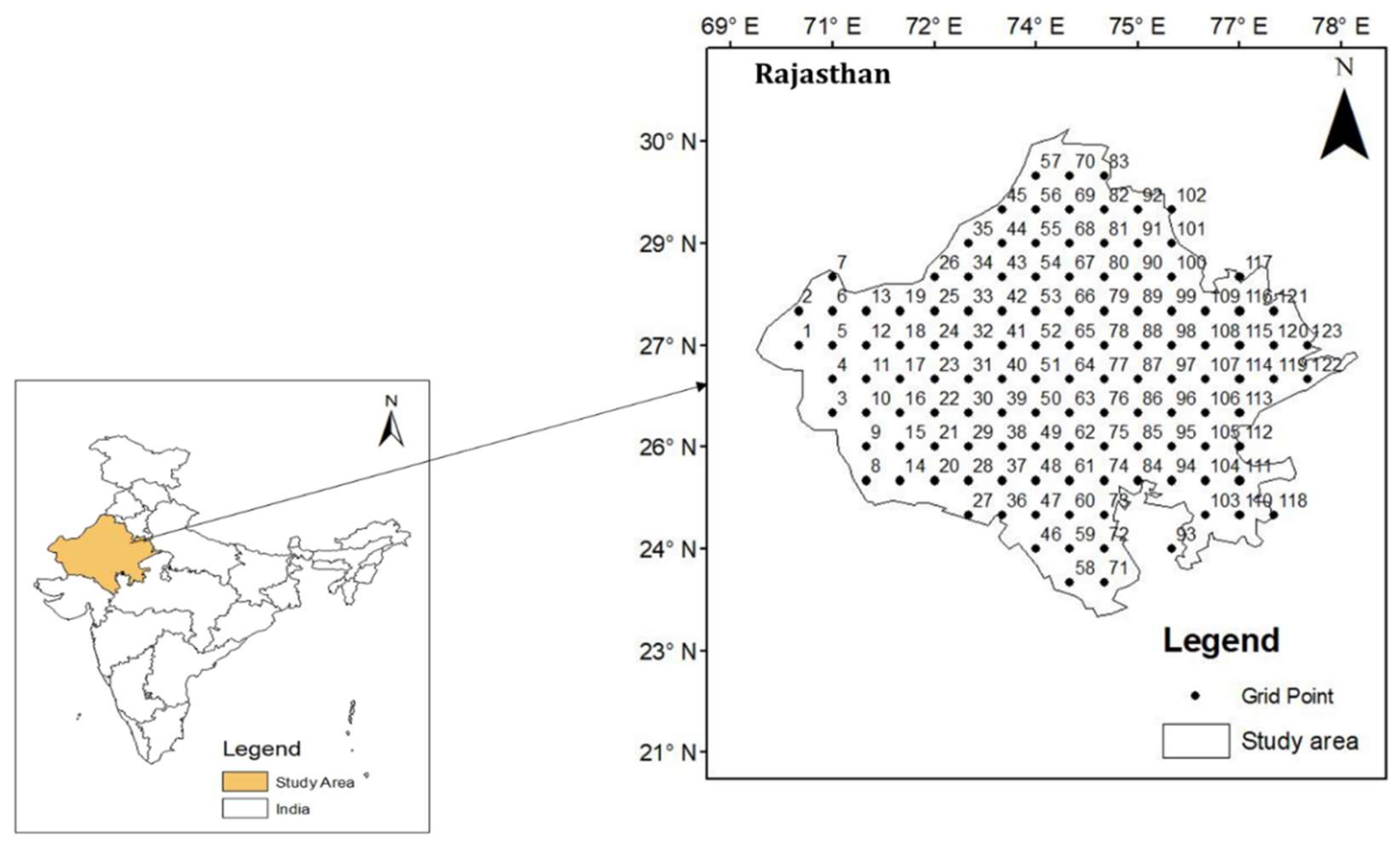
2.1. Study Area
2.2. Data Collection
3. Methods
3.1. Standard Precipitation Index (SPI)
3.2. Artificial Neural Network
3.3. Multiple Linear Regression Model
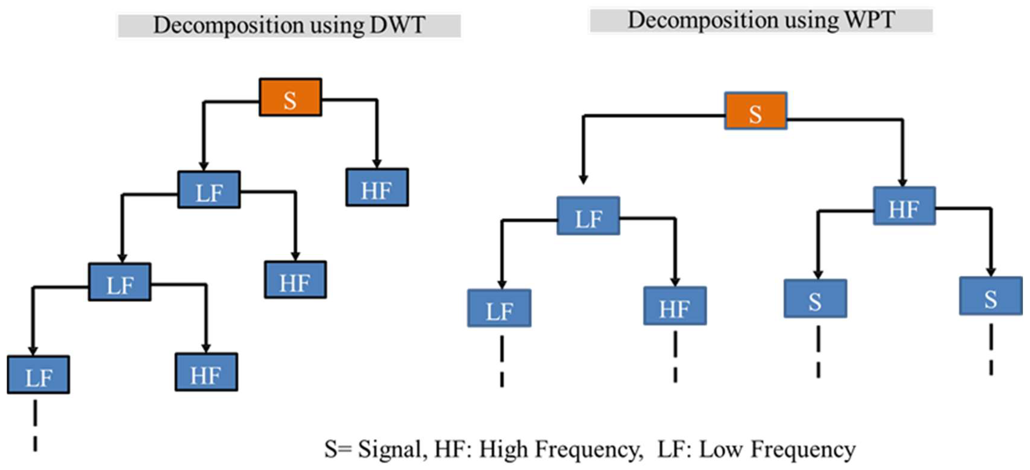
3.4. Wavelet
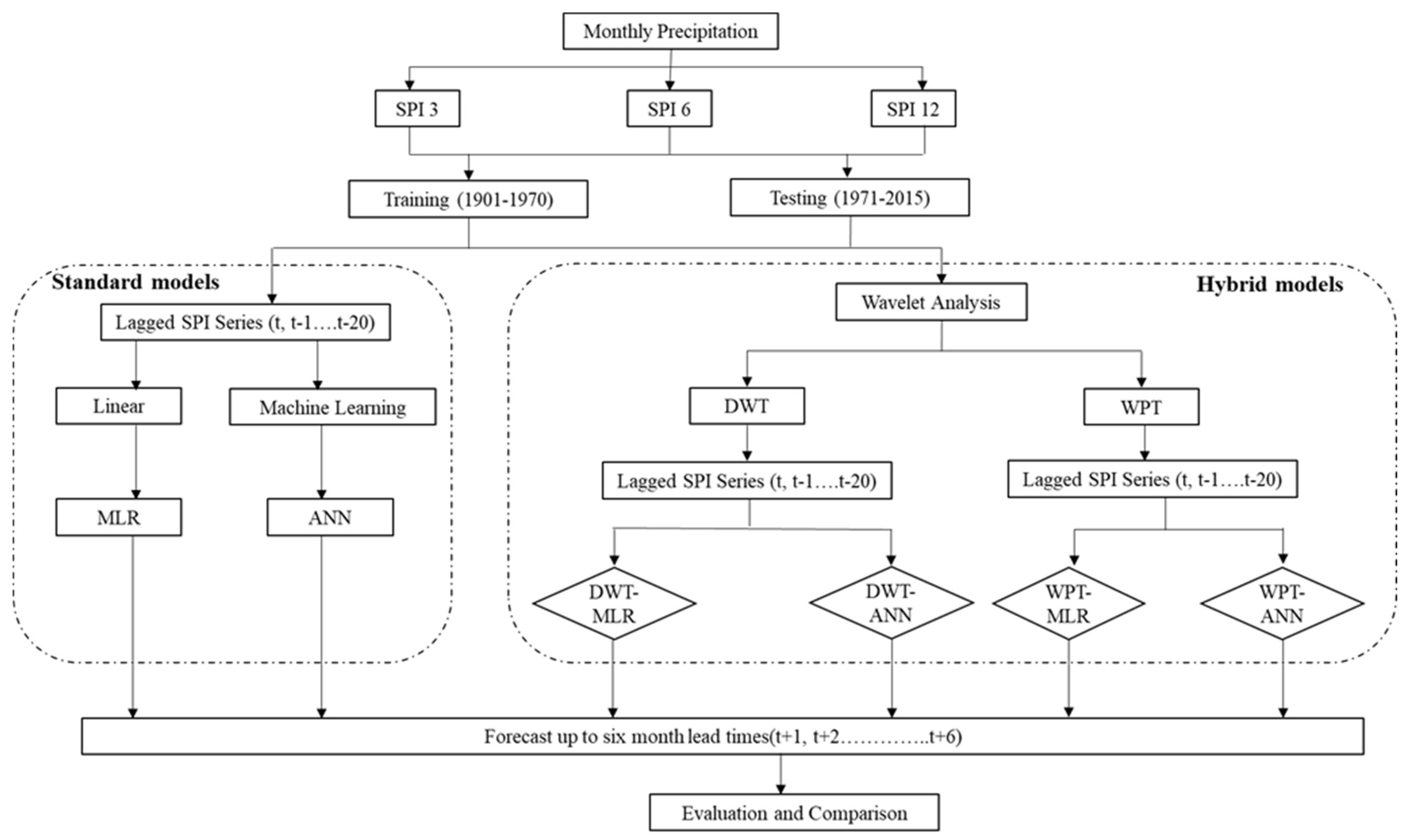
3.5. Model Development
3.6. Performance Measures
4. Results and Discussion
4.1. Artificial Neural Network Model
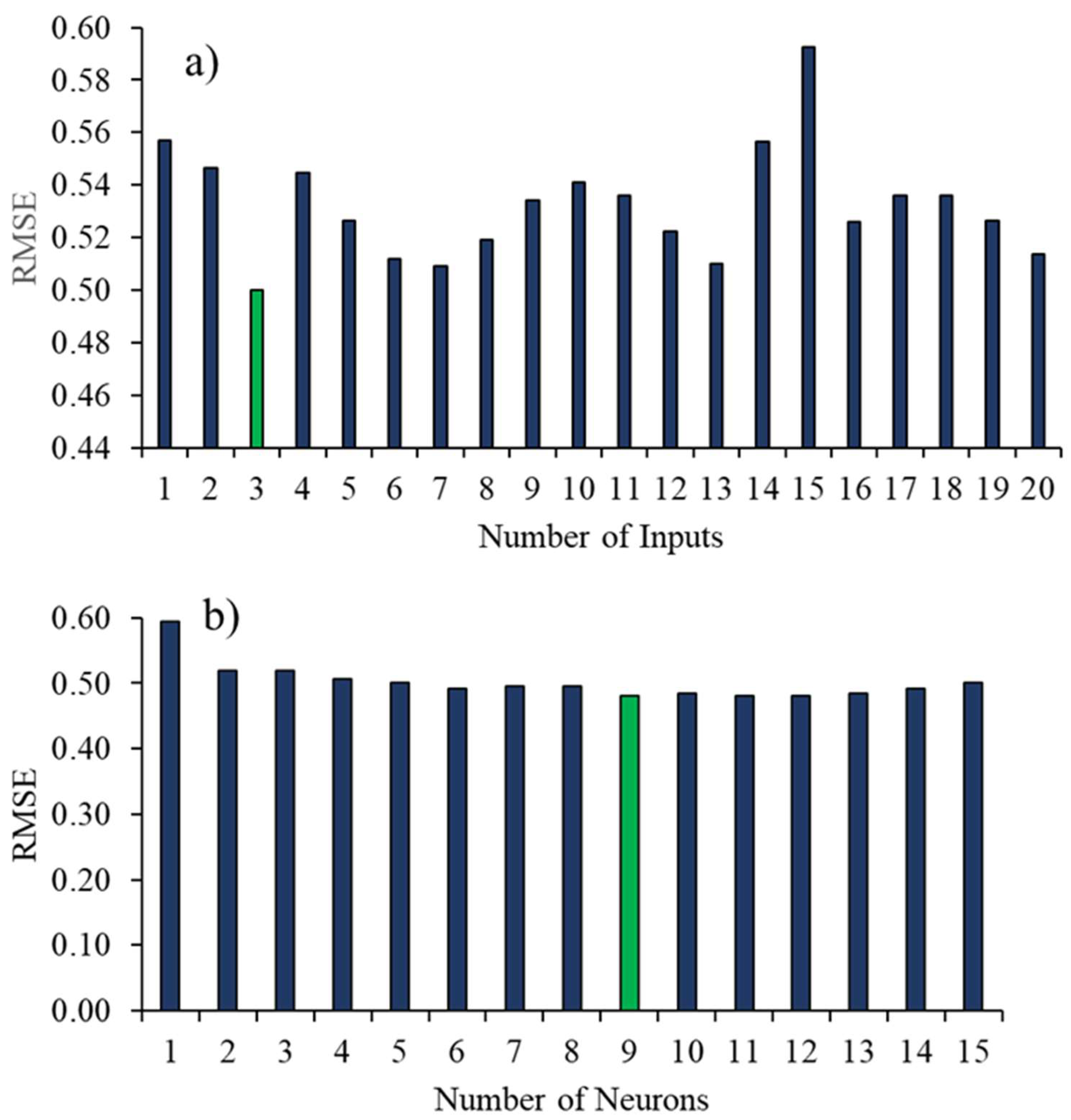
4.1.1. Selection of Artificial Neural Network Parameters
4.1.2. Performance of Artificial Neural Network Model
4.2. Performance of Multiple Linear Regression Model
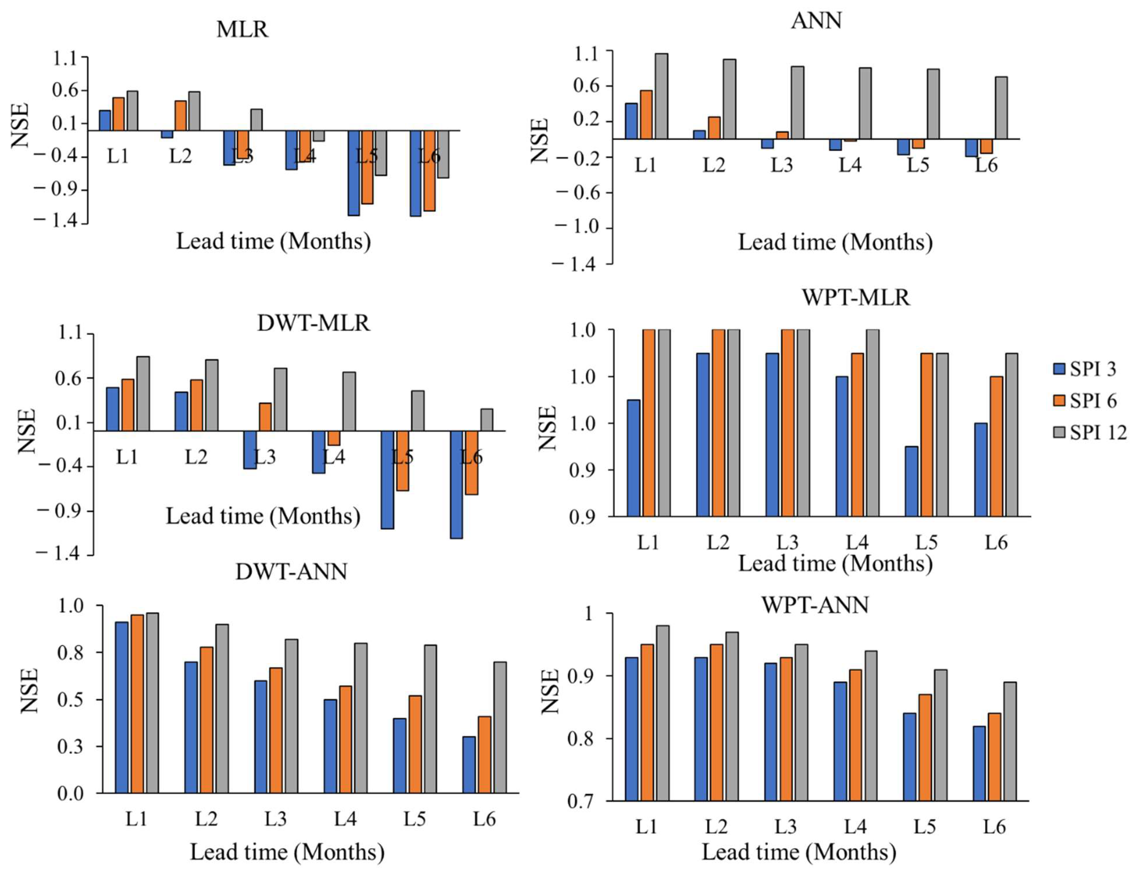
4.3. Hybrid Models
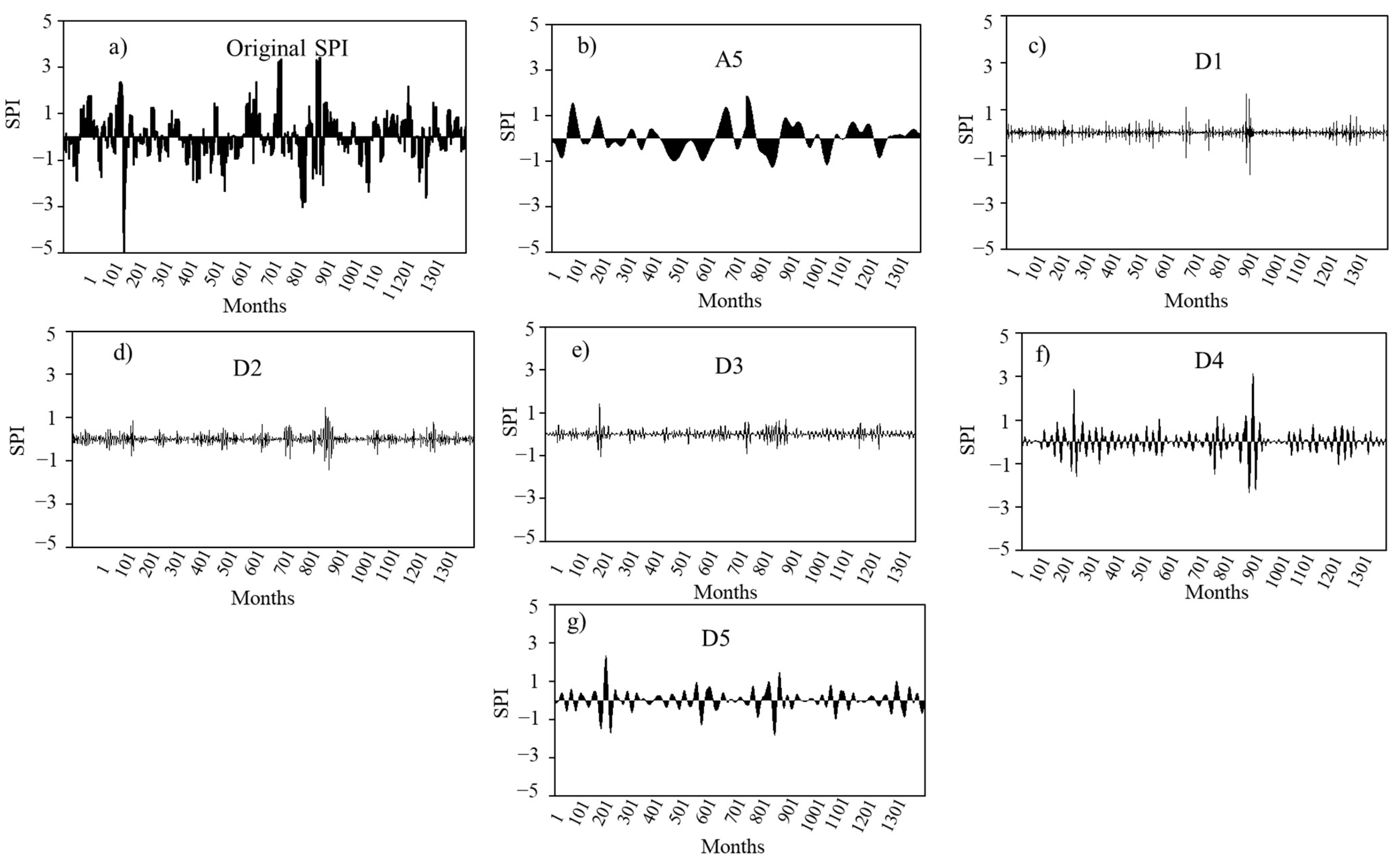
4.3.1. Selection of Wavelet Parameters
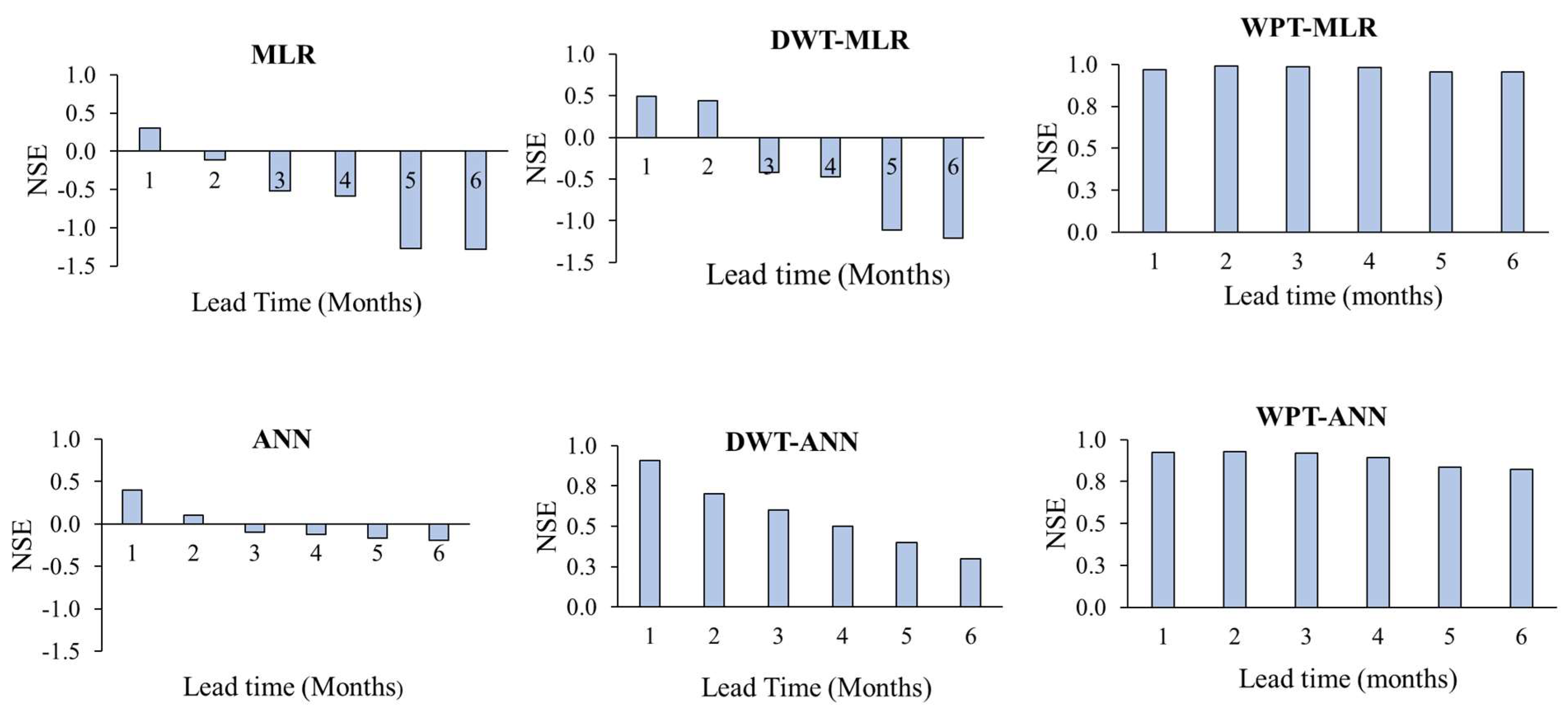
4.3.2. Performance of Hybrid Model
5. Conclusions
Supplementary Materials
Author Contributions
Funding
Data Availability Statement
Conflicts of Interest
References
- Das, P.; Naganna, S.R.; Deka, P.C.; Pushparaj, J. Hybrid wavelet packet machine learning approaches for drought modeling. Environ. Earth Sci. 2020, 79, 221. [Google Scholar] [CrossRef]
- Chang, S.; Chen, H.; Wu, B.; Nasanbat, E.; Yan, N.; Davdai, B. A practical satellite-derived vegetation drought index for arid and semi-arid grassland drought monitoring. Remote Sens. 2021, 13, 414. [Google Scholar] [CrossRef]
- Aksoy, H.; Cetin, M.; Eris, E.; Burgan, H.I.; Cavus, Y.; Yildirim, I.; Sivapalan, M. Critical drought intensity-duration-frequency curves based on total probability theorem-coupled frequency analysis. Hydrol. Sci. J. 2021, 66, 1337–1358. [Google Scholar] [CrossRef]
- Sun, P.; Ma, Z.; Zhang, Q.; Singh, V.P.; Xu, C.-Y. Modified drought severity index: Model improvement and its application in drought monitoring in China. J. Hydrol. 2022, 612, 128097. [Google Scholar] [CrossRef]
- Mishra, A.K.; Desai, V.R. Drought forecasting using feed-forward recursive neural network. Ecol. Modell. 2006, 198, 127–138. [Google Scholar] [CrossRef]
- de Brito, C.S.; da Silva, R.M.; Santos, C.A.G.; Neto, R.M.B.; Coelho, V.H.R. Monitoring meteorological drought in a semiarid region using two long-term satellite-estimated rainfall datasets: A case study of the Piranhas River basin, northeastern Brazil. Atmos. Res. 2021, 250, 105380. [Google Scholar] [CrossRef]
- Rousta, I.; Olafsson, H.; Moniruzzaman, M.; Zhang, H.; Liou, Y.-A.; Mushore, T.D.; Gupta, A. Impacts of drought on vegetation assessed by vegetation indices and meteorological factors in Afghanistan. Remote Sens. 2020, 12, 2433. [Google Scholar] [CrossRef]
- Goyal, M.K.; Sharma, A. A fuzzy c-means approach regionalization for analysis of meteorological drought homogeneous regions in western India. Nat. Hazards 2016, 84, 1831–1847. [Google Scholar] [CrossRef]
- Samra, J.S. Review and Analysis of Drought Monitoring, Declaration and Management in India; IWMI: Colombo, Sri Lanka, 2004; Volume 84, ISBN 929090576X. [Google Scholar]
- Hinge, G.; Mohamed, M.M.; Long, D.; Hamouda, M.A. Meta-Analysis in Using Satellite Precipitation Products for Drought Monitoring: Lessons Learnt and Way Forward. Remote Sens. 2021, 13, 4353. [Google Scholar] [CrossRef]
- Aghelpour, P.; Bahrami-Pichaghchi, H.; Varshavian, V. Hydrological drought forecasting using multi-scalar streamflow drought index, stochastic models and machine learning approaches, in northern Iran. Stoch. Environ. Res. Risk Assess. 2021, 35, 1615–1635. [Google Scholar] [CrossRef]
- Pai, D.S.; Sridhar, L.; Guhathakurta, P.; Hatwar, H.R. District-wide drought climatology of the southwest monsoon season over India based on standardized precipitation index (SPI). Nat. Hazards 2011, 59, 1797–1813. [Google Scholar] [CrossRef]
- Hinge, G.; Sharma, A. Comparison of wavelet and machine learning methods for regional drought prediction. In Proceedings of the EGU General Assembly Conference Abstracts, Vienna, Austria, 23–27 May 2022; p. EGU21-218. [Google Scholar]
- Jain, S.K.; Keshri, R.; Goswami, A.; Sarkar, A. Application of meteorological and vegetation indices for evaluation of drought impact: A case study for Rajasthan, India. Nat. Hazards 2010, 54, 643–656. [Google Scholar] [CrossRef]
- Stahl, K.; Kohn, I.; Blauhut, V.; Urquijo, J.; De Stefano, L.; Acácio, V.; Dias, S.; Stagge, J.H.; Tallaksen, L.M.; Kampragou, E. Impacts of European drought events: Insights from an international database of text-based reports. Nat. Hazards Earth Syst. Sci. 2016, 16, 801–819. [Google Scholar] [CrossRef] [Green Version]
- McKee, T.B.; Doesken, N.J.; Kleist, J. The relationship of drought frequency and duration to time scales. In Proceedings of the 8th Conference on Applied Climatology, Boston, MA, USA, 17–22 January 1993; Volume 17, pp. 179–183. [Google Scholar]
- Vicente-Serrano, S.M.; Beguería, S.; López-Moreno, J.I. A multiscalar drought index sensitive to global warming: The standardized precipitation evapotranspiration index. J. Clim. 2010, 23, 1696–1718. [Google Scholar] [CrossRef] [Green Version]
- Palmer, W.C. Meteorological Drought; US Department of Commerce, Weather Bureau: Washington, DC, USA, 1965; p. 58. [Google Scholar]
- Dai, A.; Trenberth, K.E.; Qian, T. A global dataset of Palmer Drought Severity Index for 1870–2002: Relationship with soil moisture and effects of surface warming. J. Hydrometeorol. 2004, 5, 1117–1130. [Google Scholar] [CrossRef] [Green Version]
- Mavromatis, T. Use of drought indices in climate change impact assessment studies: An application to Greece. Int. J. Climatol. 2010, 30, 1336–1348. [Google Scholar] [CrossRef]
- Wells, N.; Goddard, S.; Hayes, M.J. A self-calibrating Palmer drought severity index. J. Clim. 2004, 17, 2335–2351. [Google Scholar] [CrossRef]
- Palmer, W.C. Keeping track of crop moisture conditions, nationwide: The new crop moisture index. Weatherwise 1968, 21, 156–161. [Google Scholar] [CrossRef]
- Guttman, N.B. Comparing the palmer drought index and the standardized precipitation index 1. JAWRA J. Am. Water Resour. Assoc. 1998, 34, 113–121. [Google Scholar] [CrossRef]
- Mishra, A.K.; Singh, V.P. Drought modeling–A review. J. Hydrol. 2011, 403, 157–175. [Google Scholar] [CrossRef]
- Mishra, A.K.; Desai, V.R. Drought forecasting using stochastic models. Stoch. Environ. Res. Risk Assess. 2005, 19, 326–339. [Google Scholar] [CrossRef]
- Karavitis, C.A.; Vasilakou, C.G.; Tsesmelis, D.E.; Oikonomou, P.D.; Skondras, N.A.; Stamatakos, D.; Fassouli, V.; Alexandris, S. Short-term drought forecasting combining stochastic and geo-statistical approaches. Eur. Water 2015, 49, 43–63. [Google Scholar]
- Bazrafshan, O.; Salajegheh, A.; Bazrafshan, J.; Mahdavi, M.; Fatehi Maraj, A. Hydrological drought forecasting using ARIMA models (case study: Karkheh Basin). Ecopersia 2015, 3, 1099–1117. [Google Scholar]
- Han, P.; Wang, P.X.; Zhang, S.Y. Drought forecasting based on the remote sensing data using ARIMA models. Math. Comput. Model. 2010, 51, 1398–1403. [Google Scholar] [CrossRef]
- Kigumi, J.M. Use of Earth Observation Data and Artificial Neural Networks for Drought Forecasting: Case Study of Narumoro Sub-Catchment. Ph.D. Thesis, Pan African University, Addis Ababa, Ethiopia, 2018. [Google Scholar]
- Shah, H.L.; Mishra, V. Uncertainty and bias in satellite-based precipitation estimates over Indian subcontinental basins: Implications for real-time streamflow simulation and flood prediction. J. Hydrometeorol. 2016, 17, 615–636. [Google Scholar] [CrossRef]
- Nguyen, L.B.; Li, Q.F.; Ngoc, T.A.; Hiramatsu, K. Adaptive Neuro–Fuzzy Inference System for Drought Forecasting in the Cai River Basin in Vietnam. J. Fac. Agric. Kyushu Univ. 2015, 60, 405–415. [Google Scholar] [CrossRef]
- Morid, S.; Smakhtin, V.; Bagherzadeh, K. Drought forecasting using artificial neural networks and time series of drought indices. Int. J. Climatol. A J. R. Meteorol. Soc. 2007, 27, 2103–2111. [Google Scholar] [CrossRef]
- Dai, A. Drought under global warming: A review. Wiley Interdiscip. Rev. Clim. Chang. 2011, 2, 45–65. [Google Scholar] [CrossRef] [Green Version]
- Belayneh, A.; Adamowski, J.; Khalil, B.; Ozga-Zielinski, B. Long-term SPI drought forecasting in the Awash River Basin in Ethiopia using wavelet neural network and wavelet support vector regression models. J. Hydrol. 2014, 508, 418–429. [Google Scholar] [CrossRef]
- Belayneh, A.; Adamowski, J.; Khalil, B. Short-term SPI drought forecasting in the Awash River Basin in Ethiopia using wavelet transforms and machine learning methods. Sustain. Water Resour. Manag. 2016, 2, 87–101. [Google Scholar] [CrossRef]
- Kim, T.-W.; Valdés, J.B. Nonlinear model for drought forecasting based on a conjunction of wavelet transforms and neural networks. J. Hydrol. Eng. 2003, 8, 319–328. [Google Scholar] [CrossRef] [Green Version]
- Maity, R.; Suman, M.; Verma, N.K. Drought prediction using a wavelet based approach to model the temporal consequences of different types of droughts. J. Hydrol. 2016, 539, 417–428. [Google Scholar] [CrossRef]
- Djerbouai, S.; Souag-Gamane, D. Drought forecasting using neural networks, wavelet neural networks, and stochastic models: Case of the Algerois Basin in North Algeria. Water Resour. Manag. 2016, 30, 2445–2464. [Google Scholar] [CrossRef]
- Mehr, A.D.; Kahya, E.; Özger, M. A gene–wavelet model for long lead time drought forecasting. J. Hydrol. 2014, 517, 691–699. [Google Scholar] [CrossRef]
- Deo, R.C.; Tiwari, M.K.; Adamowski, J.F.; Quilty, J.M. Forecasting effective drought index using a wavelet extreme learning machine (W-ELM) model. Stoch. Environ. Res. Risk Assess. 2017, 31, 1211–1240. [Google Scholar] [CrossRef]
- Belayneh, A.; Adamowski, J. Standard precipitation index drought forecasting using neural networks, wavelet neural networks, and support vector regression. Appl. Comput. Intell. Soft Comput. 2012, 2012, 794061. [Google Scholar] [CrossRef] [Green Version]
- Komasi, M.; Sharghi, S.; Safavi, H.R. Wavelet and cuckoo search-support vector machine conjugation for drought forecasting using Standardized Precipitation Index (case study: Urmia Lake, Iran). J. Hydroinform. 2018, 20, 975–988. [Google Scholar] [CrossRef] [Green Version]
- Peel, M.C.; Finlayson, B.L.; McMahon, T.A. Updated world map of the Köppen-Geiger climate classification. Hydrol. Earth Syst. Sci. 2007, 11, 1633–1644. [Google Scholar] [CrossRef] [Green Version]
- Mundetia, N.; Sharma, D. Analysis of rainfall and drought in Rajasthan State, India. Glob. Nest J 2015, 17, 12–21. [Google Scholar]
- Mishra, D.; Goswami, S.; Matin, S.; Sarup, J. Analyzing the extent of drought in the Rajasthan state of India using vegetation condition index and standardized precipitation index. Model. Earth Syst. Environ. 2022, 8, 601–610. [Google Scholar] [CrossRef]
- Rajeevan, M.; Bhate, J. A high resolution daily gridded rainfall dataset (1971–2005) for mesoscale meteorological studies. Curr. Sci. 2009, 96, 558–562. [Google Scholar]
- Adane, G.B.; Hirpa, B.A.; Song, C.; Lee, W.-K. Rainfall characterization and trend analysis of wet spell length across varied landscapes of the Upper Awash River Basin, Ethiopia. Sustainability 2020, 12, 9221. [Google Scholar] [CrossRef]
- GUIDE; WMO Standardized Precipitation Index User; Svoboda, M.; Hayes, M.; Wood, D. World Meteorological Organization: Geneva; WMO: Geneva, Switzerland, 2012. [Google Scholar]
- Agatonovic-Kustrin, S.; Beresford, R. Basic concepts of artificial neural network (ANN) modeling and its application in pharmaceutical research. J. Pharm. Biomed. Anal. 2000, 22, 717–727. [Google Scholar] [CrossRef] [PubMed]
- Kukreja, H.; Bharath, N.; Siddesh, C.S.; Kuldeep, S. An introduction to artificial neural network. Int. J. Adv. Res. Innov. Ideas Educ. 2016, 1, 27–30. [Google Scholar]
- Brace, M.C.; Schmidt, J.; Hadlin, M. Comparison of the forecasting accuracy of neural networks with other established techniques. In Proceedings of the First International Forum on Applications of Neural Networks to Power Systems, Singapore, 18-21 November 1991; pp. 31–35. [Google Scholar]
- Chandwani, V.; Agrawal, V.; Nagar, R. Applications of soft computing in civil engineering: A review. Int. J. Comput. Appl. 2013, 81, 13–20. [Google Scholar] [CrossRef]
- Tranmer, M.; Elliot, M. Multiple linear regression. Cathie Marsh Cent. Census Surv. Res. 2008, 5, 1–5. [Google Scholar]
- Grossmann, A.; Morlet, J. Decomposition of Hardy functions into square integrable wavelets of constant shape. SIAM J. Math. Anal. 1984, 15, 723–736. [Google Scholar] [CrossRef] [Green Version]
- Özger, M.; Mishra, A.K.; Singh, V.P. Long lead time drought forecasting using a wavelet and fuzzy logic combination model: A case study in Texas. J. Hydrometeorol. 2012, 13, 284–297. [Google Scholar] [CrossRef]
- Kişi, Ö. Wavelet regression model as an alternative to neural networks for monthly streamflow forecasting. Hydrol. Process. Int. J. 2009, 23, 3583–3597. [Google Scholar] [CrossRef]
- Maheswaran, R.; Khosa, R. Comparative study of different wavelets for hydrologic forecasting. Comput. Geosci. 2012, 46, 284–295. [Google Scholar] [CrossRef]
- Joshi, N.; Gupta, D.; Suryavanshi, S.; Adamowski, J.; Madramootoo, C.A. Analysis of trends and dominant periodicities in drought variables in India: A wavelet transform based approach. Atmos. Res. 2016, 182, 200–220. [Google Scholar] [CrossRef]
- Khan, M.M.H.; Muhammad, N.S.; El-Shafie, A. Wavelet based hybrid ANN-ARIMA models for meteorological drought forecasting. J. Hydrol. 2020, 590, 125380. [Google Scholar] [CrossRef]
- Sharma, A.; Goyal, M.K. Assessment of drought trend and variability in India using wavelet transform. Hydrol. Sci. J. 2020, 65, 1539–1554. [Google Scholar] [CrossRef]
- Rizal, A.; Hidayat, R.; Nugroho, H.A. Comparison of discrete wavelet transform and wavelet packet decomposition for the lung sound classification. Far East J. Electron. Commun. 2017, 17, 1065–1078. [Google Scholar] [CrossRef]
- Nourani, V.; Baghanam, A.H.; Adamowski, J.; Kisi, O. Applications of hybrid wavelet–artificial intelligence models in hydrology: A review. J. Hydrol. 2014, 514, 358–377. [Google Scholar] [CrossRef]


| SPI Value | Classification |
|---|---|
| >2 | Extremely wet |
| 1.50 to1.99 | Very Wet |
| 1.00 to1.49 | Moderately wet |
| −0.99 to 0.99 | Near Normal |
| −1.0 to −1.49 | Moderately dry |
| −1.5 to −1.99 | Severely dry |
| <−2.0 | Extremely dry |
| Model | Model Description |
|---|---|
| MLR | |
| ANN | |
| DWT-MLR | |
| DWT-ANN | |
| WPT-MLR | |
| WPT-ANN |
| Lead Time (Months) | Statistic | ANN Model | MLR Model | ||||
|---|---|---|---|---|---|---|---|
| SPI-3 | SPI-6 | SPI-12 | SPI-3 | SPI-6 | SPI-12 | ||
| 1 | RMSE | 0.7 | 0.66 | 0.3 | 0.93 | 0.86 | 0.76 |
| NSE | 0.4 | 0.55 | 0.9 | 0.3 | 0.49 | 0.59 | |
| MAE | 0.6 | 0.48 | 0.2 | 0.69 | 0.54 | 0.30 | |
| 2 | RMSE | 0.9 | 0.85 | 0.5 | 1.23 | 0.58 | 0.54 |
| NSE | 0.1 | 0.25 | 0.7 | −0.11 | 0.44 | 0.58 | |
| MAE | 0.7 | 0.65 | 0.3 | 0.75 | 0.59 | 0.39 | |
| 3 | RMSE | 1.01 | 0.95 | 0.7 | 1.32 | 0.72 | 0.62 |
| NSE | −0.10 | 0.08 | 0.5 | −0.52 | −0.42 | 0.32 | |
| MAE | 0.80 | 0.74 | 0.4 | 0.79 | 0.60 | 0.48 | |
| 4 | RMSE | 1.09 | 0.99 | 0.70 | 1.37 | 0.73 | 0.70 |
| NSE | −0.12 | −0.02 | 0.5 | −0.59 | −0.47 | −0.16 | |
| MAE | 0.81 | 0.79 | 0.5 | 0.85 | 0.65 | 0.52 | |
| 5 | RMSE | 1.10 | 1.03 | 0.8 | 1.45 | 0.77 | 0.75 |
| NSE | −0.17 | −0.10 | 0.4 | −1.27 | −1.10 | −0.67 | |
| MAE | 0.82 | 0.80 | 0.60 | 0.87 | 0.72 | 0.69 | |
| 6 | RMSE | 1.29 | 1.07 | 0.8 | 1.59 | 0.78 | 0.74 |
| NSE | −0.19 | −0.16 | 0.3 | −1.28 | −1.21 | −0.71 | |
| MAE | 0.83 | 0.81 | 0.63 | 0.88 | 0.73 | 0.68 | |
| Mother Wavelet (dbn) | |||||||||||||||||||||
|---|---|---|---|---|---|---|---|---|---|---|---|---|---|---|---|---|---|---|---|---|---|
| 1 | 2 | 3 | 4 | 5 | 6 | 7 | 8 | 9 | 10 | 11 | 12 | 13 | 14 | 15 | 16 | 17 | 18 | 19 | 20 | ||
| Level of Decomposition | 1 | 0.557 | 0.546 | 0.553 | 0.545 | 0.527 | 0.512 | 0.509 | 0.519 | 0.534 | 0.541 | 0.536 | 0.522 | 0.510 | 0.506 | 0.512 | 0.526 | 0.536 | 0.536 | 0.526 | 0.514 |
| 2 | 0.540 | 0.517 | 0.521 | 0.520 | 0.491 | 0.480 | 0.491 | 0.496 | 0.495 | 0.512 | 0.504 | 0.481 | 0.482 | 0.487 | 0.482 | 0.494 | 0.508 | 0.496 | 0.489 | 0.488 | |
| 3 | 0.542 | 0.519 | 0.518 | 0.518 | 0.490 | 0.479 | 0.487 | 0.494 | 0.494 | 0.508 | 0.501 | 0.478 | 0.480 | 0.483 | 0.482 | 0.491 | 0.506 | 0.493 | 0.488 | 0.484 | |
| 4 | 0.542 | 0.519 | 0.518 | 0.518 | 0.492 | 0.479 | 0.487 | 0.495 | 0.494 | 0.509 | 0.501 | 0.479 | 0.480 | 0.484 | 0.482 | 0.491 | 0.506 | 0.494 | 0.488 | 0.484 | |
| 5 | 0.543 | 0.519 | 0.518 | 0.518 | 0.492 | 0.480 | 0.487 | 0.495 | 0.495 | 0.509 | 0.502 | 0.480 | 0.480 | 0.484 | 0.482 | 0.491 | 0.506 | 0.494 | 0.488 | 0.484 | |
| 6 | 0.544 | 0.519 | 0.518 | 0.519 | 0.492 | 0.480 | 0.487 | 0.496 | 0.495 | 0.509 | 0.502 | 0.480 | 0.480 | 0.484 | 0.482 | 0.491 | 0.506 | 0.494 | 0.488 | 0.484 | |
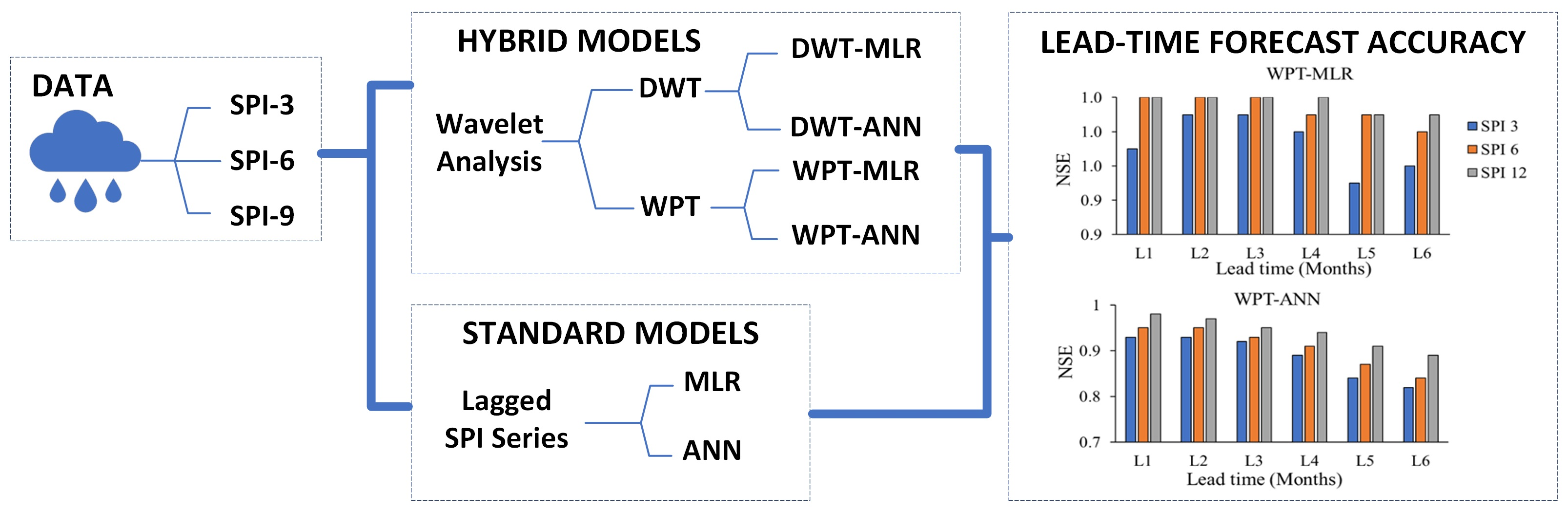
| Lead Time (Months) | Statistic | SPI-3 | SPI-6 | SPI-12 | |||||||||
|---|---|---|---|---|---|---|---|---|---|---|---|---|---|
| DWT-MLR | WPT-MLR | DWT-ANN | WPT-ANN | DWT-MLR | WPT-MLR | DWT-ANN | WPT-ANN | DWT-MLR | WPT-MLR | DWT-ANN | WPT-ANN | ||
| 1 | RMSE | 0.56 | 0.17 | 0.28 | 0.26 | 0.76 | 0.04 | 0.22 | 0.15 | 0.83 | 0.03 | 0.19 | 0.13 |
| NSE | 0.49 | 0.97 | 0.91 | 0.93 | 0.59 | 1 | 0.95 | 0.95 | 0.84 | 1 | 0.96 | 0.98 | |
| MAE | 0.21 | 0.07 | 0.18 | 0.15 | 0.19 | 0.05 | 0.13 | 0.13 | 0.17 | 0.03 | 0.10 | 0.12 | |
| 2 | RMSE | 0.58 | 0.09 | 0.49 | 0.25 | 0.54 | 0.03 | 0.46 | 0.23 | 0.77 | 0.03 | 0.3 | 0.17 |
| NSE | 0.44 | 0.99 | 0.7 | 0.93 | 0.58 | 1 | 0.78 | 0.95 | 0.81 | 1 | 0.9 | 0.97 | |
| MAE | 0.22 | 0.08 | 0.19 | 0.17 | 0.25 | 0.06 | 0.19 | 0.15 | 0.21 | 0.04 | 0.13 | 0.13 | |
| 3 | RMSE | 0.72 | 0.11 | 0.6 | 0.26 | 0.62 | 0.05 | 0.55 | 0.26 | 0.43 | 0.03 | 0.40 | 0.22 |
| NSE | −0.42 | 0.99 | 0.6 | 0.92 | 0.32 | 1 | 0.67 | 0.93 | 0.71 | 1 | 0.82 | 0.95 | |
| MAE | 0.25 | 0.08 | 0.23 | 0.18 | 0.27 | 0.07 | 0.23 | 0.16 | 0.23 | 0.05 | 0.18 | 0.14 | |
| 4 | RMSE | 0.73 | 0.13 | 0.70 | 0.31 | 0.70 | 0.07 | 0.64 | 0.3 | 0.48 | 0.04 | 0.40 | 0.23 |
| NSE | −0.47 | 0.98 | 0.5 | 0.89 | −0.16 | 0.99 | 0.57 | 0.91 | 0.67 | 1 | 0.8 | 0.94 | |
| MAE | 0.32 | 0.09 | 0.27 | 0.19 | 0.28 | 0.08 | 0.29 | 0.17 | 0.28 | 0.07 | 0.19 | 0.15 | |
| 5 | RMSE | 0.77 | 0.2 | 0.70 | 0.38 | 0.75 | 0.11 | 0.70 | 0.35 | 0.57 | 0.07 | 0.40 | 0.28 |
| NSE | −1.10 | 0.95 | 0.4 | 0.84 | −0.67 | 0.99 | 0.52 | 0.87 | 0.46 | 0.99 | 0.79 | 0.91 | |
| MAE | 0.36 | 0.10 | 0.28 | 0.19 | 0.29 | 0.09 | 0.30 | 0.18 | 0.28 | 0.08 | 0.20 | 0.17 | |
| 6 | RMSE | 0.78 | 0.2 | 0.80 | 0.4 | 0.74 | 0.14 | 0.76 | 0.39 | 0.63 | 0.09 | 0.50 | 0.32 |
| NSE | −1.21 | 0.96 | 0.30 | 0.82 | −0.71 | 0.98 | 0.41 | 0.84 | 0.25 | 0.99 | 0.70 | 0.89 | |
| MAE | 0.38 | 0.10 | 0.29 | 0.20 | 0.30 | 0.09 | 0.30 | 0.19 | 0.29 | 0.08 | 0.20 | 0.18 | |
Publisher’s Note: MDPI stays neutral with regard to jurisdictional claims in published maps and institutional affiliations. |
© 2022 by the authors. Licensee MDPI, Basel, Switzerland. This article is an open access article distributed under the terms and conditions of the Creative Commons Attribution (CC BY) license (https://creativecommons.org/licenses/by/4.0/).
Share and Cite
Hinge, G.; Piplodiya, J.; Sharma, A.; Hamouda, M.A.; Mohamed, M.M. Evaluation of Hybrid Wavelet Models for Regional Drought Forecasting. Remote Sens. 2022, 14, 6381. https://doi.org/10.3390/rs14246381
Hinge G, Piplodiya J, Sharma A, Hamouda MA, Mohamed MM. Evaluation of Hybrid Wavelet Models for Regional Drought Forecasting. Remote Sensing. 2022; 14(24):6381. https://doi.org/10.3390/rs14246381
Chicago/Turabian StyleHinge, Gilbert, Jay Piplodiya, Ashutosh Sharma, Mohamed A. Hamouda, and Mohamed M. Mohamed. 2022. "Evaluation of Hybrid Wavelet Models for Regional Drought Forecasting" Remote Sensing 14, no. 24: 6381. https://doi.org/10.3390/rs14246381