
Estimation of Urban Forest Characteristic Parameters Using UAV-Lidar Coupled with Canopy Volume


 , ,
, ,
Abstract
:1. Introduction
2. Materials and Methods
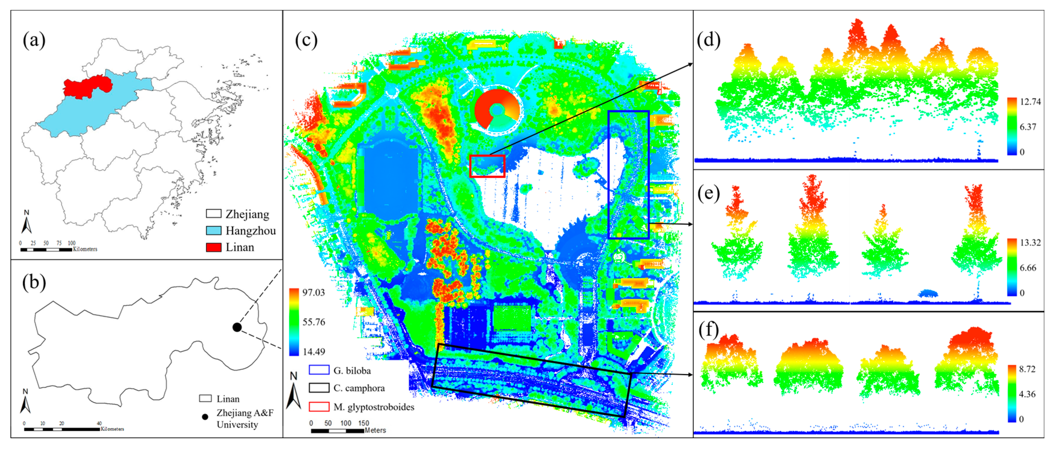
2.1. Study Area
2.2. Field Measurements
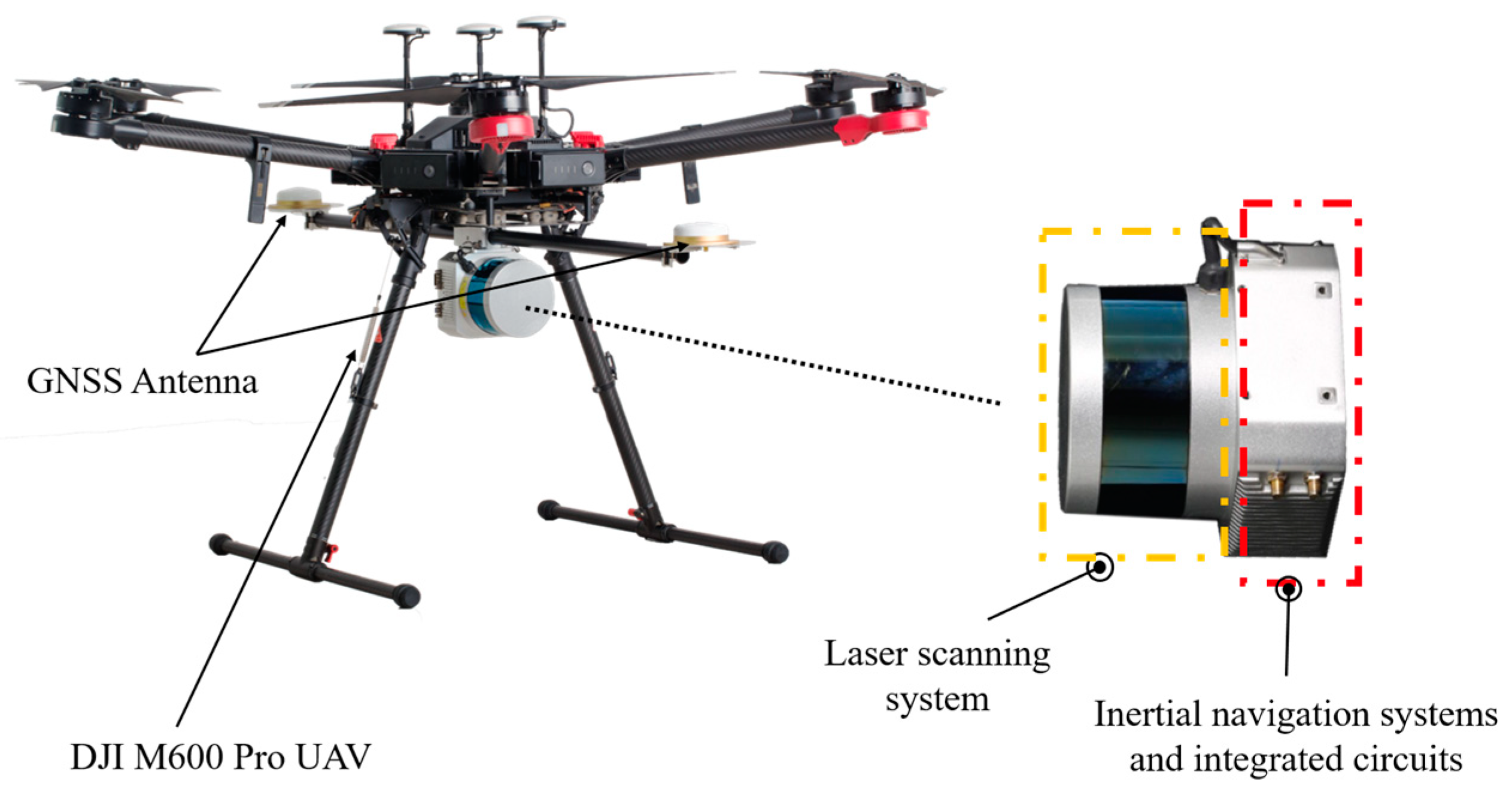
2.3. Lidar Data
2.3.1. Lidar Data Preprocessing
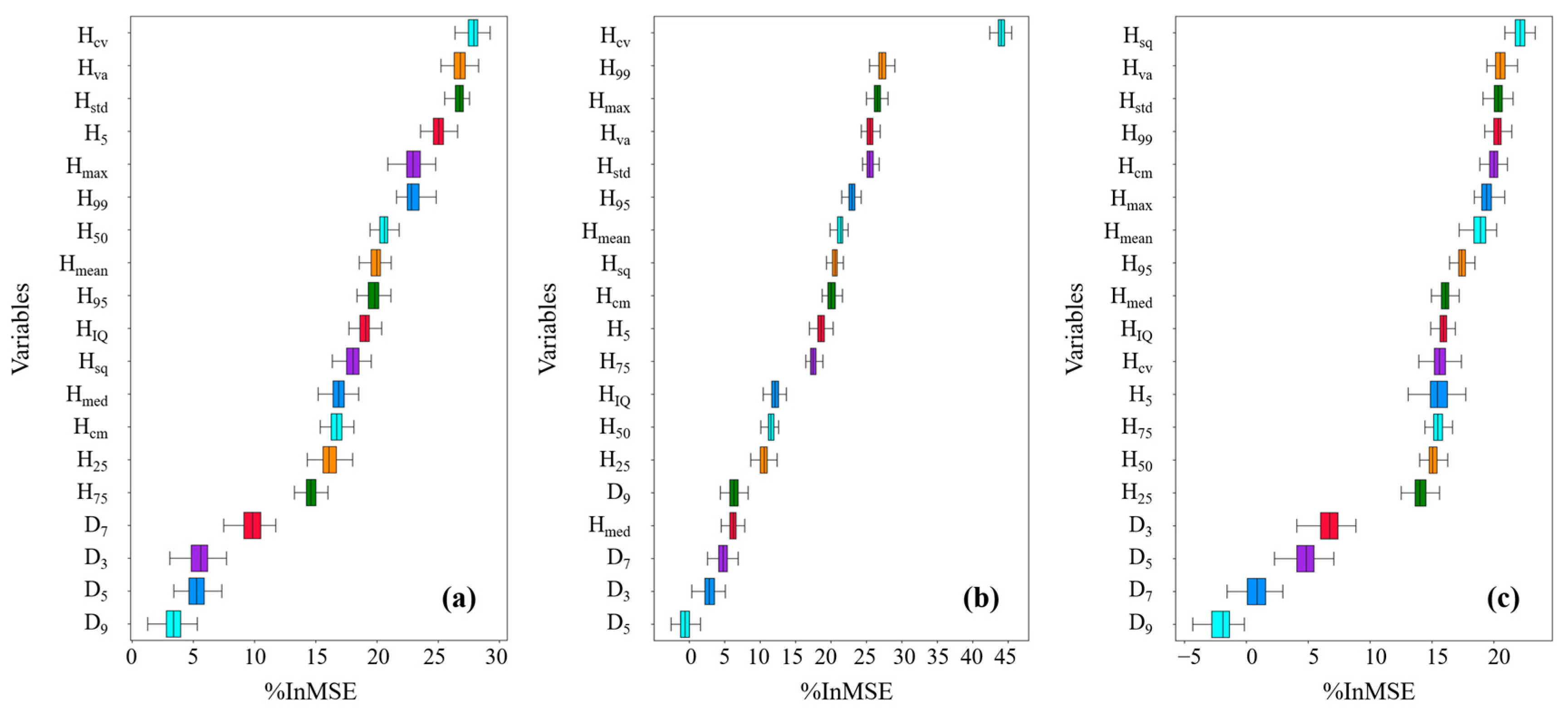
2.3.2. Lidar Metrics
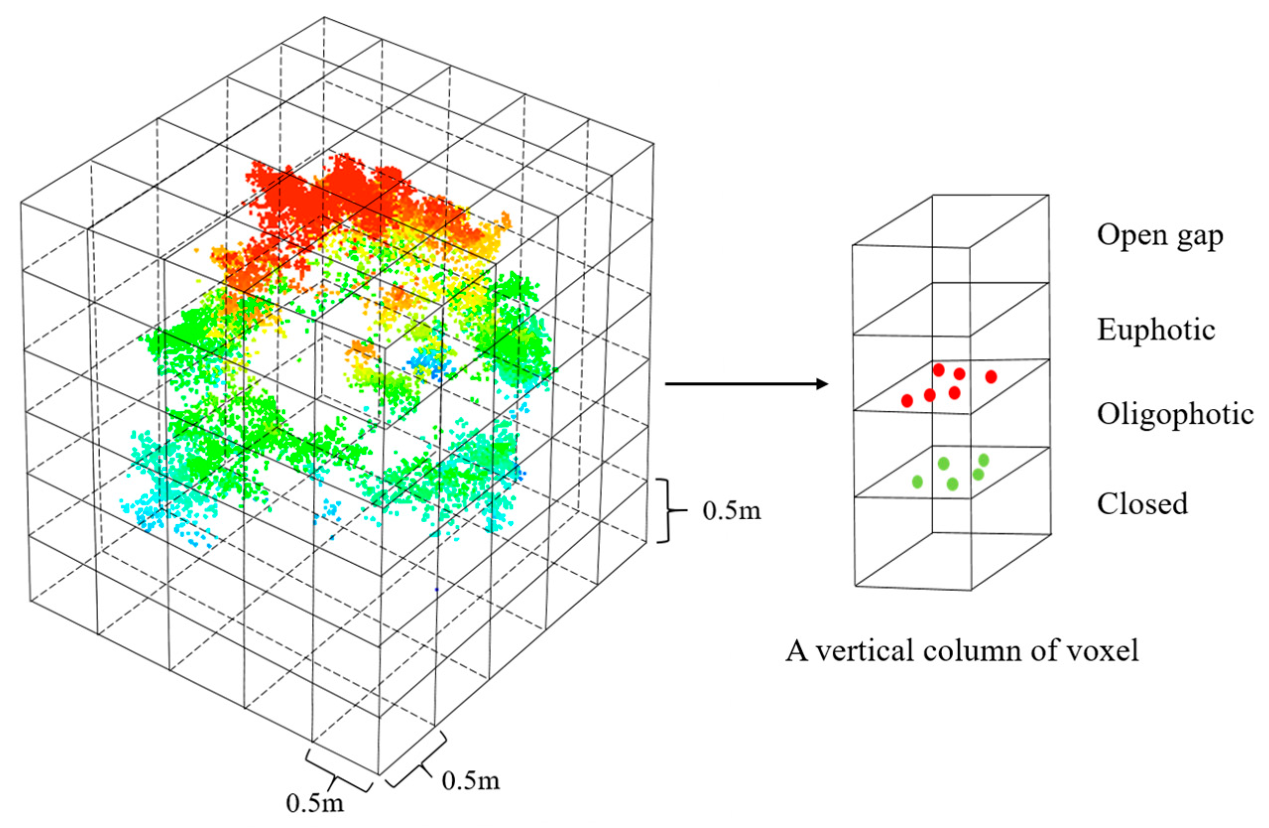
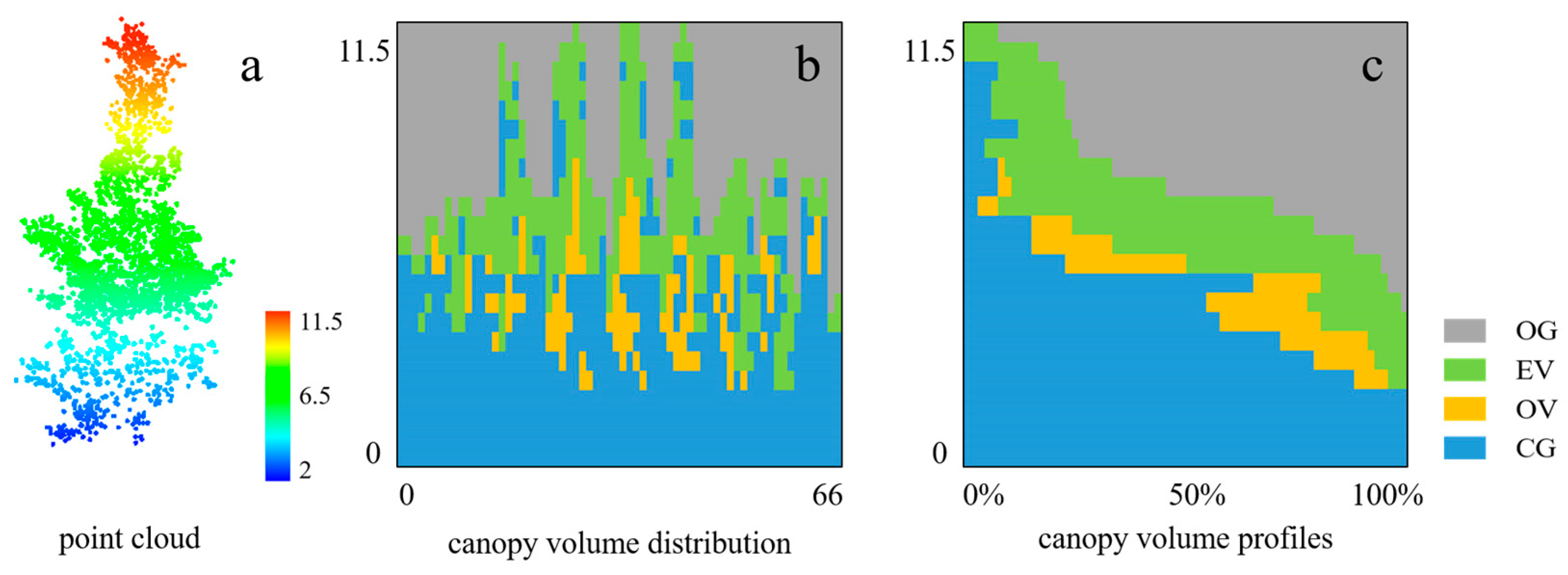
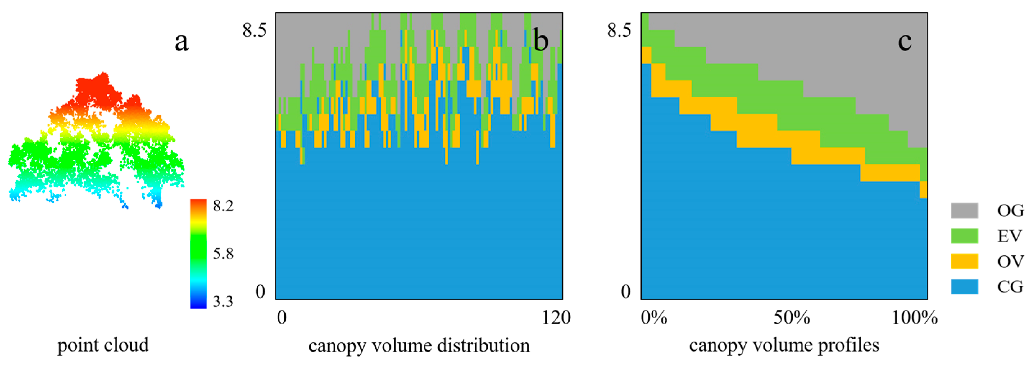
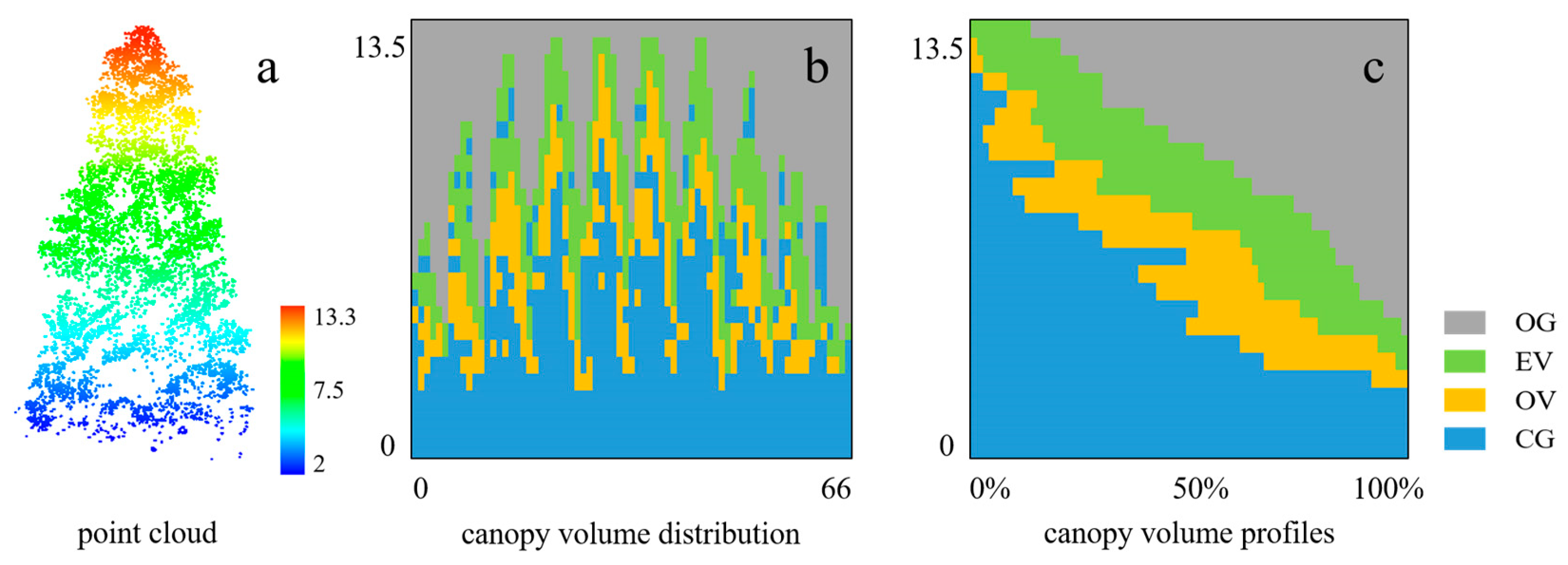
2.3.3. Calculation of the Volume of Single Tree Canopy

| Metrics | Description | Reference | |
|---|---|---|---|
| Height-based metrics(HB) | Height percentiles (H5, H25, H50, H75, H95, and H99) | The percentiles of the canopy height distribution (5th, 25th, 50th, 75th, 95th, and 99th) of first returns | [25,45,46] |
| The coefficient of variation of height (Hcv) | The coefficient of variation of heights of all first returns | ||
| Maximum height (Hmax) | Maximum height above ground of all first returns | ||
| Variance of height (Hva) | The variation in heights of all first returns | ||
| Standard deviation of height (Hstd) | The standard deviation of heights of all first returns | ||
| Median height (Hmed) | Median height above ground of all first returns | ||
| Mean height (Hmean) | Mean height above ground of all first returns | ||
| Interquartile distance of height (HIQ) | The interquartile distance of height of all first returns | ||
| Root mean square of height (Hsq) | The root mean square of height of all first returns | ||
| Cube mean of height (Hcm) | The cube mean of height of all first returns | ||
| Density-based metrics(DB) | Canopy return density (D3, D5, D7, D9) | The proportion of points above the quantiles (30th, 50th, 70th and 90th) to total number of points | [47] |
| Canopy structure metrics(CS) | Canopy projection area (S) | Canopy projection area calculated using two-dimensional convex hull algorithm | [21] |
| Crown diameter (CD) | Average diameter of crown point cloud | ||
| Open gap volume (OG) and closed gap volume (CG) of CVM | The volume of empty voxels located above and below the filled canopy, respectively | [32] | |
| Euphotic volume (EV) and oligophotic volume (OV) of CVM | The volume of filled voxels located 65% above and 35% below of all filled grid cells of that column |
2.4. Model Construction Methods and Scheme
2.4.1. MLR Model
2.4.2. SVR Model
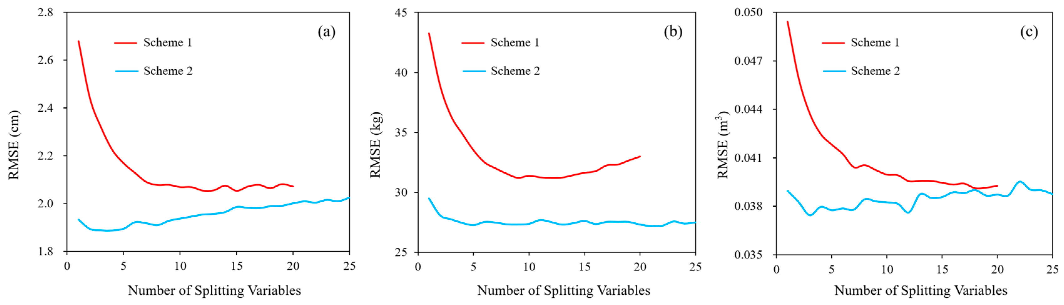
2.4.3. RF Model
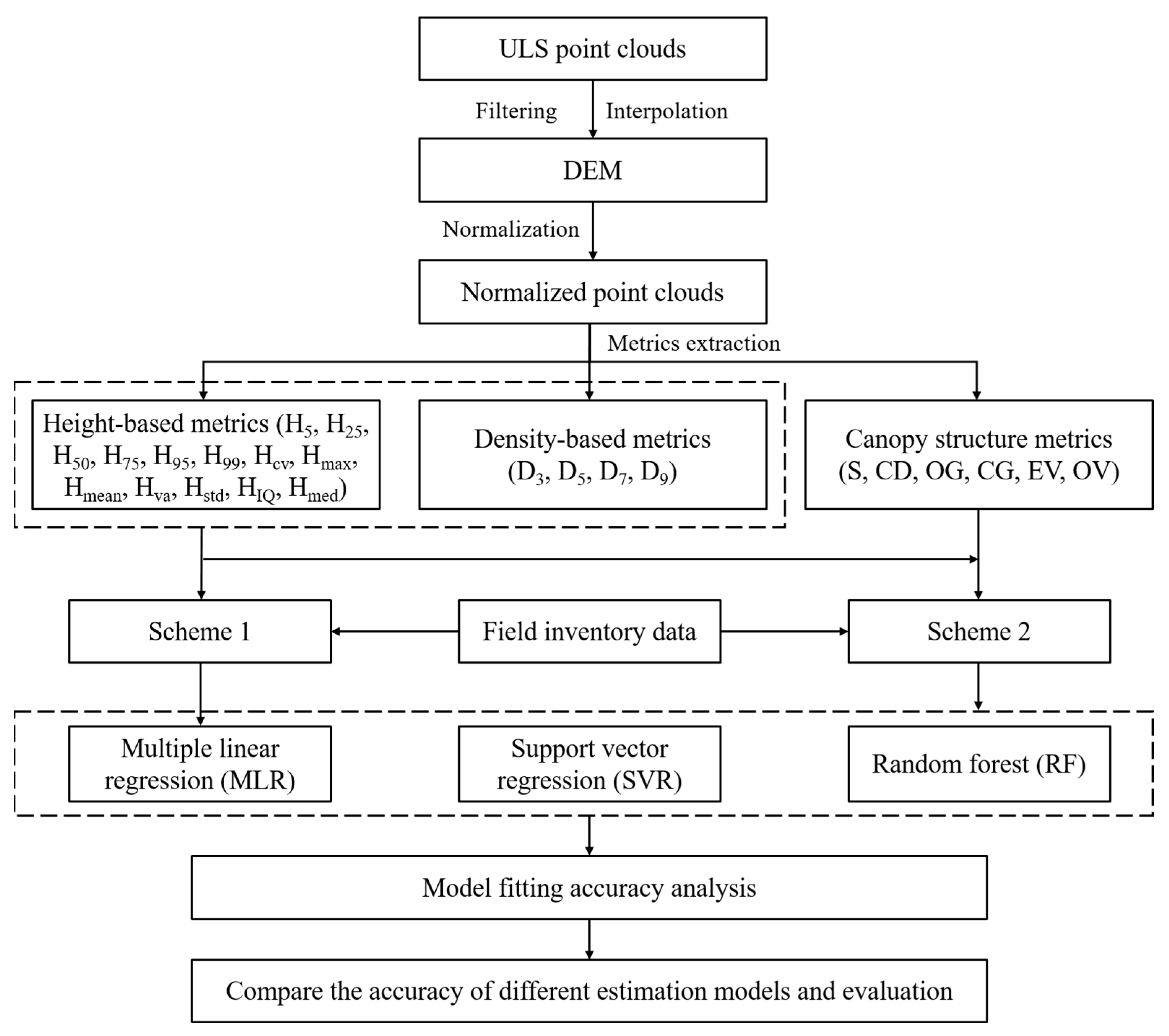
2.5. The Flow Chart and Accuracy Validation
3. Results
3.1. Canopy Volume and Profile Analysis
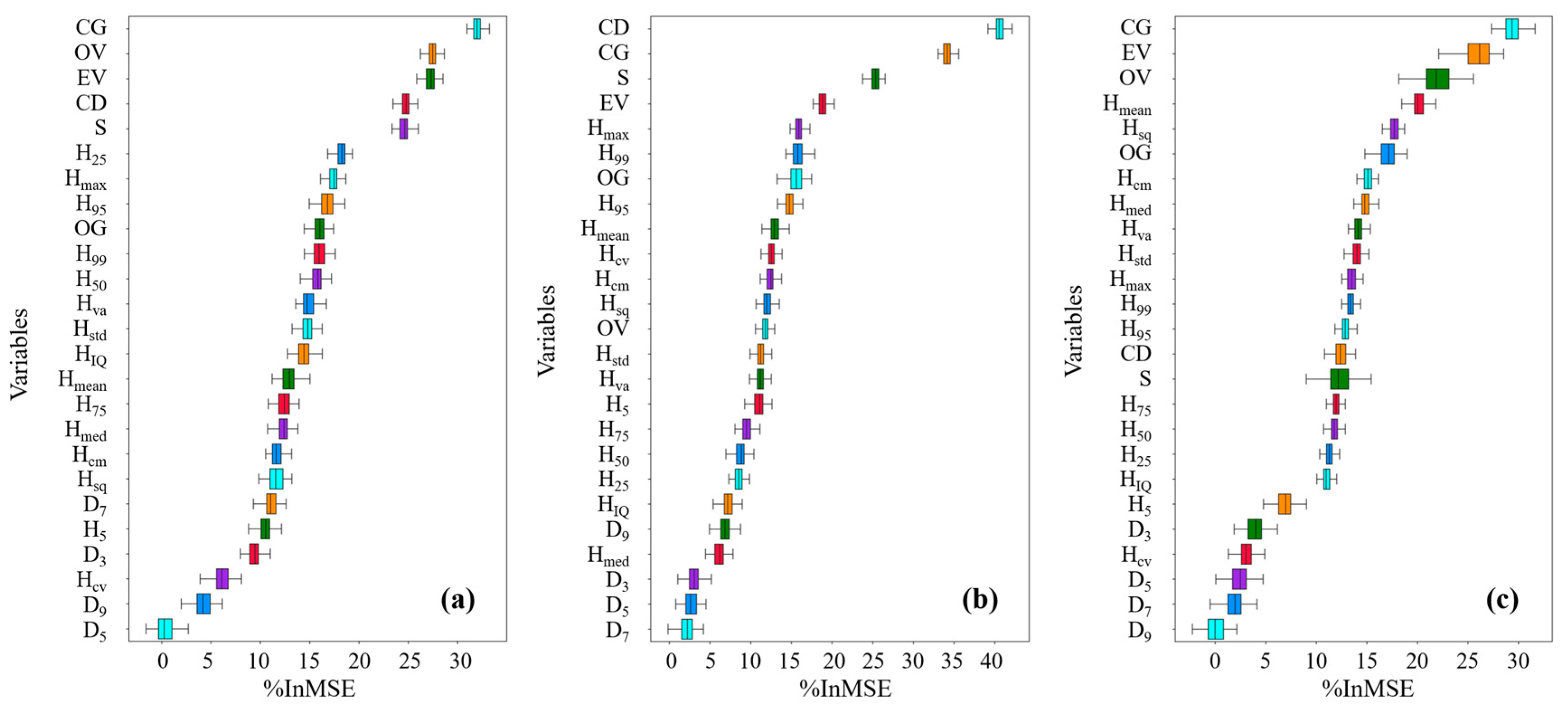
3.2. Variable Importance Analysis
3.3. Model Construction and Evaluation
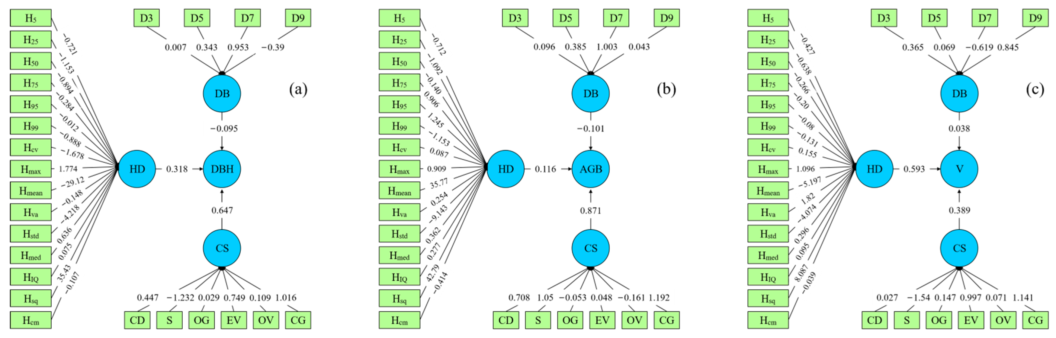
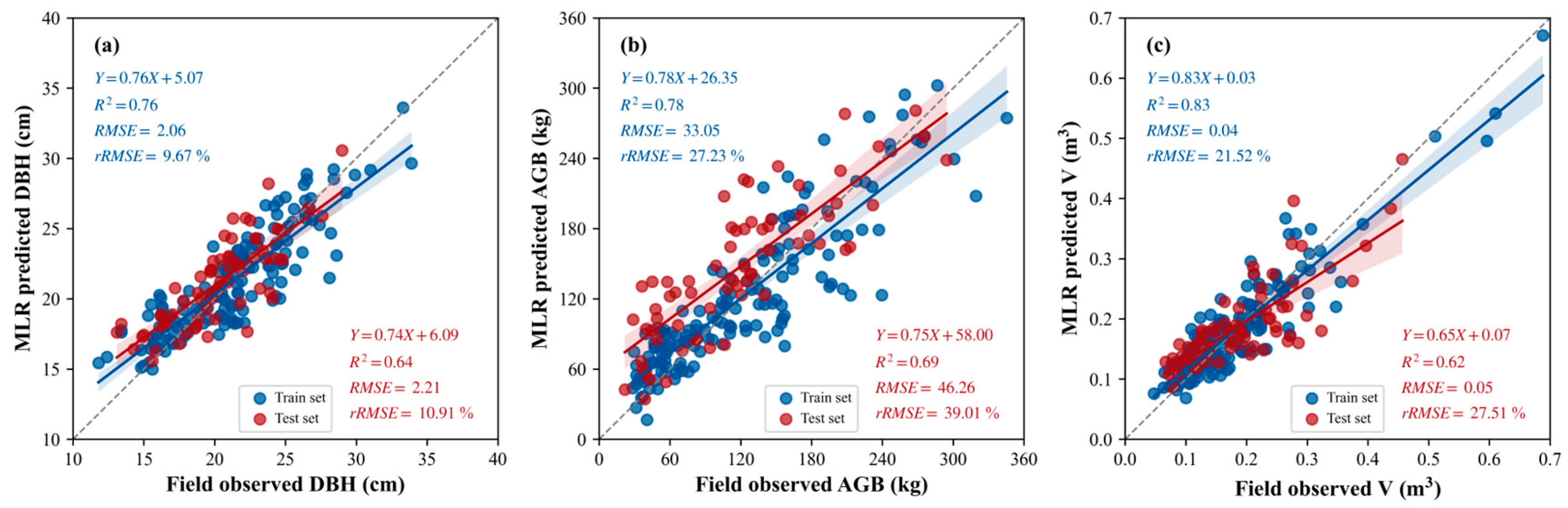
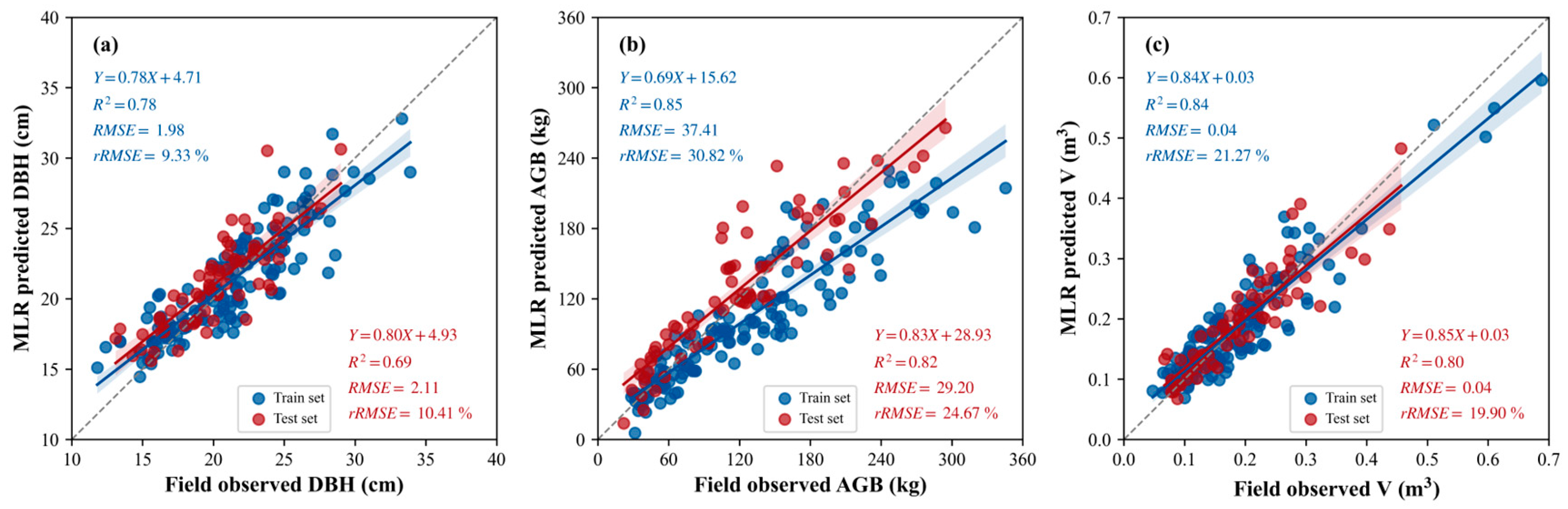
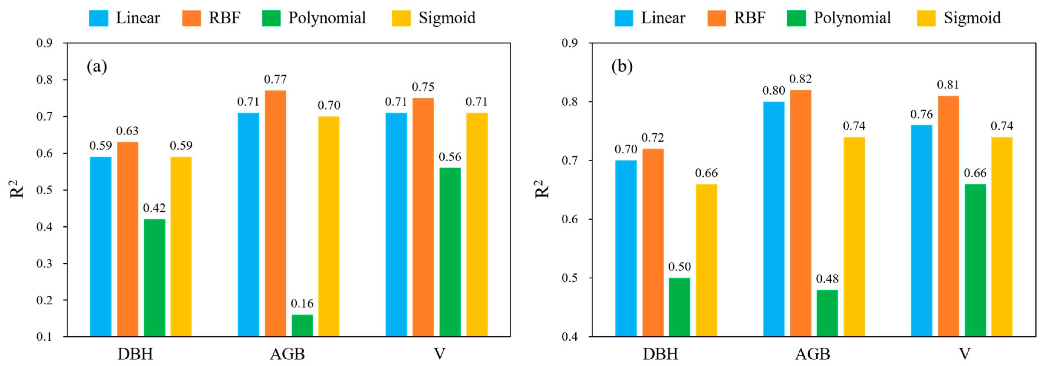
3.3.1. MLR Estimation Results
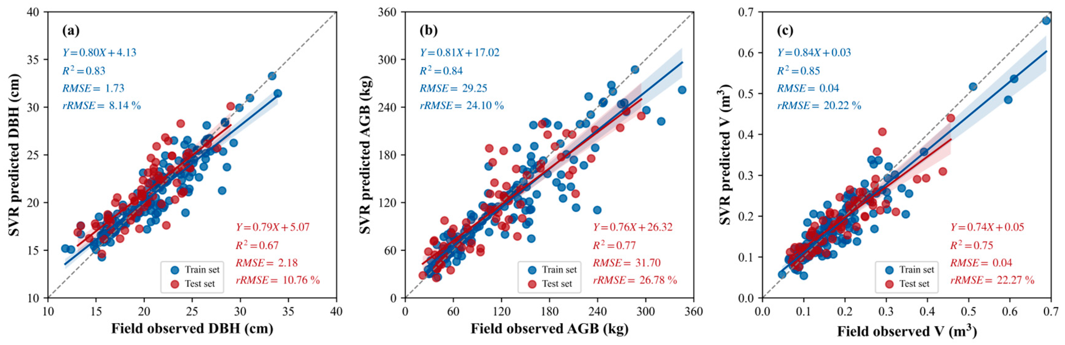
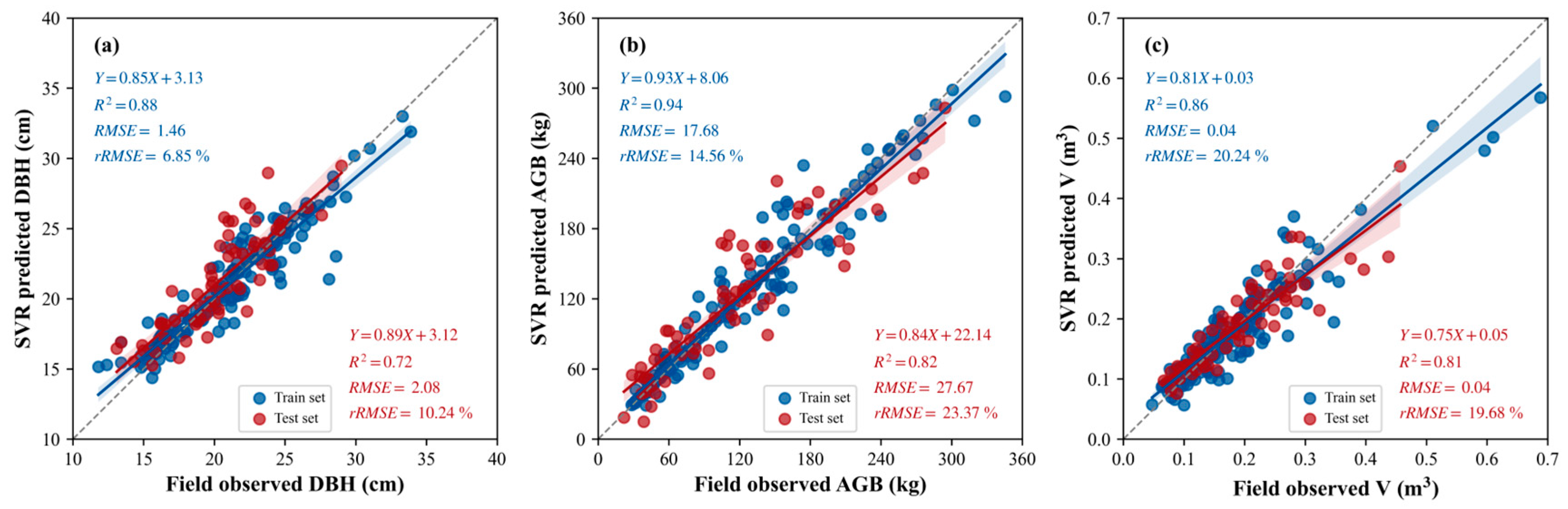
3.3.2. SVR Estimation Results
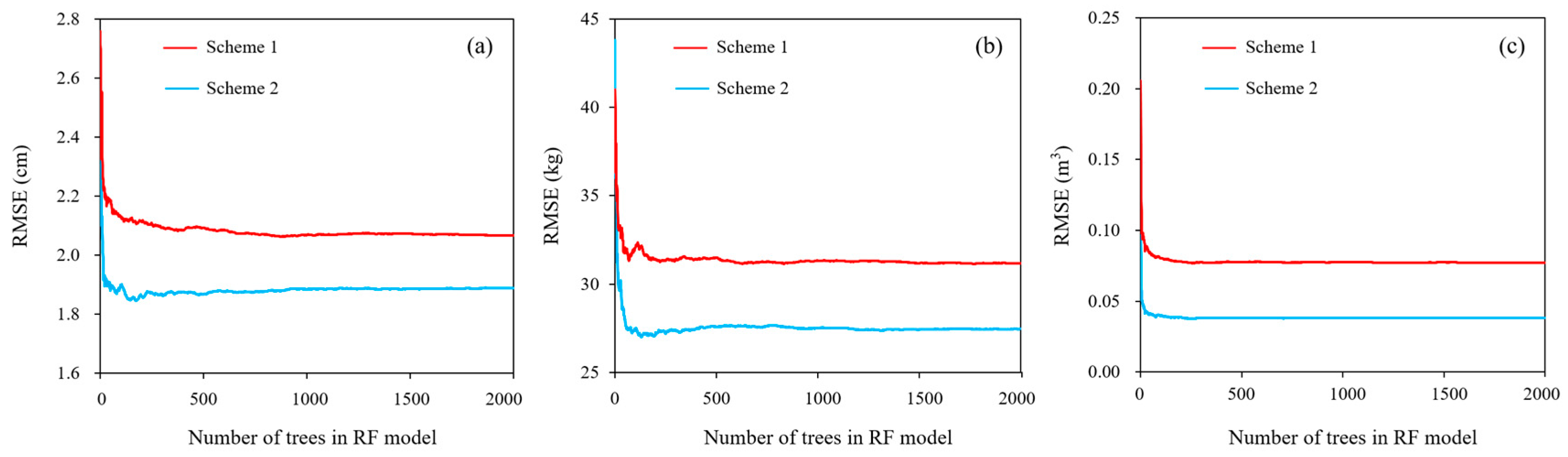
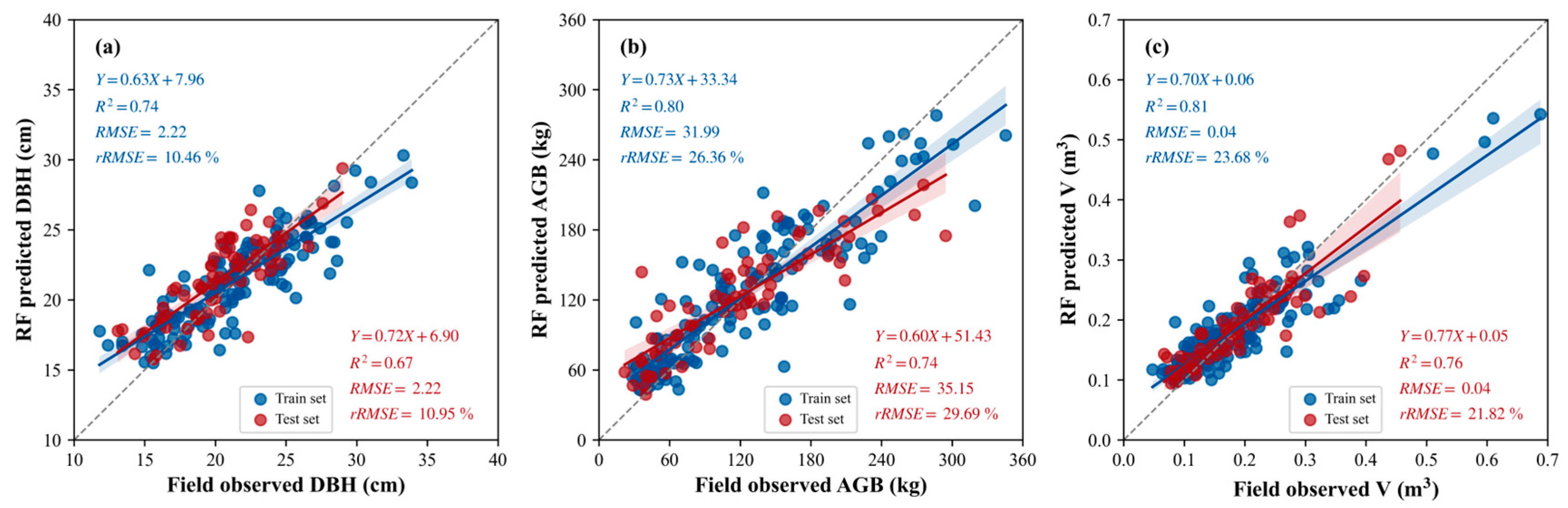
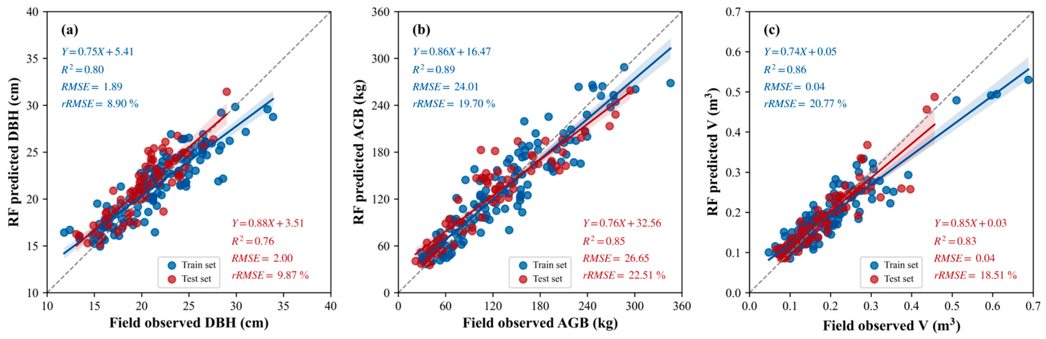
3.3.3. RF Estimation Results
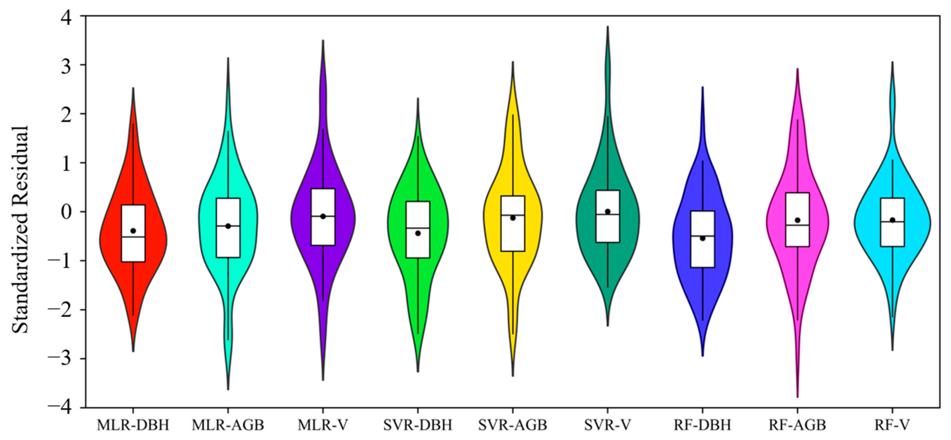
3.4. Comparison of Model Results
4. Discussion
5. Conclusions
Author Contributions
Funding
Data Availability Statement
Acknowledgments
Conflicts of Interest
Appendix A
| Model | Scheme | DBH | AGB | V | |||||||
|---|---|---|---|---|---|---|---|---|---|---|---|
| R2 | RMSE | rRMSE (%) | R2 | RMSE | rRMSE (%) | R2 | RMSE | rRMSE (%) | |||
| Train | MLR | Scheme 1 | 0.76 | 2.06 | 9.67 | 0.78 | 33.05 | 27.23 | 0.83 | 0.04 | 21.52 |
| Scheme 2 | 0.78 | 1.98 | 9.33 | 0.85 | 37.41 | 30.82 | 0.84 | 0.04 | 21.27 | ||
| SVR | Scheme 1 | 0.83 | 1.73 | 8.14 | 0.84 | 29.25 | 24.10 | 0.85 | 0.04 | 20.22 | |
| Scheme 2 | 0.88 | 1.46 | 6.85 | 0.94 | 17.68 | 14.56 | 0.86 | 0.04 | 20.24 | ||
| RF | Scheme 1 | 0.74 | 2.22 | 10.46 | 0.80 | 31.99 | 26.36 | 0.81 | 0.04 | 23.68 | |
| Scheme 2 | 0.80 | 1.89 | 8.90 | 0.89 | 24.01 | 19.70 | 0.86 | 0.04 | 20.77 | ||
| Test | MLR | Scheme 1 | 0.64 | 2.21 | 10.91 | 0.69 | 46.26 | 39.01 | 0.62 | 0.05 | 27.51 |
| Scheme 2 | 0.69 | 2.11 | 10.41 | 0.82 | 29.20 | 24.67 | 0.80 | 0.04 | 19.90 | ||
| SVR | Scheme 1 | 0.67 | 2.18 | 10.76 | 0.77 | 31.70 | 26.78 | 0.75 | 0.04 | 22.27 | |
| Scheme 2 | 0.72 | 2.08 | 10.24 | 0.82 | 27.67 | 23.37 | 0.81 | 0.04 | 19.68 | ||
| RF | Scheme 1 | 0.67 | 2.22 | 10.95 | 0.74 | 35.15 | 29.69 | 0.76 | 0.04 | 21.82 | |
| Scheme 2 | 0.76 | 2.00 | 9.87 | 0.85 | 26.65 | 22.51 | 0.83 | 0.04 | 18.51 | ||
References
- Baumeister, C.F.; Gerstenberg, T.; Plieninger, T.; Schraml, U. Exploring cultural ecosystem service hotspots: Linking multiple urban forest features with public participation mapping data. Urban For. Urban Green. 2020, 48, 126561. [Google Scholar] [CrossRef]
- Cheng, W.; Chunju, C.; Kanghua, T. The Concept, Range and Researh Area of Urban Forest. World For. Res. 2004, 17, 23–27. [Google Scholar] [CrossRef]
- Escobedo, F.J.; Nowak, D.J. Spatial heterogeneity and air pollution removal by an urban forest. Landsc. Urban Plan 2009, 90, 102–110. [Google Scholar] [CrossRef]
- Liu, L.; Coops, N.C.; Aven, N.W.; Pang, Y. Mapping urban tree species using integrated airborne hyperspectral and LiDAR remote sensing data. Remote Sens. Environ. 2017, 200, 170–182. [Google Scholar] [CrossRef]
- Zengyuan, L.; Qingwang, L.; Yong, P. Review on forest parameters inversion using LiDAR. Natl. Remote Sens. Bull. 2016, 20, 1138–1150. [Google Scholar]
- Jones, M.S.D. Characterizing forest ecological structure using pulse types and heights of airborne laser scanning. Remote Sens. Environ. 2010, 114, 1069–1076. [Google Scholar]
- Li, X.; Liu, J.; Jiang, S.; Jia, B. Analysis of the urban tree canopy and community structure of hospitals in urban areas of Beijing. Acta Ecol. Sin. 2019, 39, 12. [Google Scholar]
- Wang, C.; Peng, Z.; Tao, K. Characteristics and development of urban forest in China. Chin. J. Ecol. 2004, 23, 5. [Google Scholar]
- Gao, L.; Chai, G.; Zhang, X. Above-Ground Biomass Estimation of Plantation with Different Tree Species Using Airborne LiDAR and Hyperspectral Data. Remote Sens. 2022, 14, 2568. [Google Scholar] [CrossRef]
- Wulder, M.A.; White, J.C.; Nelson, R.F.; Nsset, E.; Gobakken, T. LiDAR sampling for large-area forest characterization: A review. Remote Sens. Environ. 2012, 121, 196–209. [Google Scholar] [CrossRef] [Green Version]
- Hirata, Y.; Furuya, N.; Saito, H.; Pak, C.; Leng, C.; Sokh, H.; Ma, V.; Kajisa, T.; Ota, T.; Mizoue, N. Object-Based Mapping of Aboveground Biomass in Tropical Forests Using LiDAR and Very-High-Spatial-Resolution Satellite Data. Remote Sens. 2018, 10, 438. [Google Scholar] [CrossRef] [Green Version]
- Torres de Almeida, C.; Gerente, J.; Rodrigo dos Prazeres Campos, J.; Caruso Gomes Junior, F.; Providelo, L.A.; Marchiori, G.; Chen, X. Canopy Height Mapping by Sentinel 1 and 2 Satellite Images, Airborne LiDAR Data, and Machine Learning. Remote Sens. 2022, 14, 4112. [Google Scholar] [CrossRef]
- Cao, L.; Coops, N.C.; Sun, Y.; Ruan, H.; Wang, G.; Dai, J.; She, G. Estimating canopy structure and biomass in bamboo forests using airborne LiDAR data. ISPRS J. Photogramm. Remote Sens. 2019, 148, 114–129. [Google Scholar] [CrossRef]
- Yin, T.; Cook, B.D.; Morton, D.C. Three-dimensional estimation of deciduous forest canopy structure and leaf area using multi-directional, leaf-on and leaf-off airborne lidar data. Agric. For. Meteorol. 2022, 314, 108781. [Google Scholar] [CrossRef]
- Zhao, Y.; Liu, X.; Wang, Y.; Zheng, Z.; Zheng, S.; Zhao, D.; Bai, Y. UAV-based individual shrub aboveground biomass estimation calibrated against terrestrial LiDAR in a shrub-encroached grassland. Int. J. Appl. Earth Obs. Geoinf. 2021, 101, 102358. [Google Scholar] [CrossRef]
- Jiang, X.; Li, G.; Lu, D.; Chen, E.; Wei, X. Stratification-Based Forest Aboveground Biomass Estimation in a Subtropical Region Using Airborne Lidar Data. Remote Sens. 2020, 12, 1101. [Google Scholar] [CrossRef] [Green Version]
- Lin, W.; Lu, Y.; Li, G.; Jiang, X.; Lu, D. A comparative analysis of modeling approaches and canopy height-based data sources for mapping forest growing stock volume in a northern subtropical ecosystem of China. GIScience Remote Sens. 2022, 59, 568–589. [Google Scholar] [CrossRef]
- Nguyen, T.H.; Jones, S.D.; Soto-Berelov, M.; Haywood, A.; Hislop, S. Monitoring aboveground forest biomass dynamics over three decades using Landsat time-series and single-date inventory data. Int. J. Appl. Earth Obs. Geoinf. 2020, 84, 101952. [Google Scholar] [CrossRef]
- Zhao, K.; Suarez, J.C.; Garcia, M.; Hu, T.; Wang, C.; Londo, A. Utility of multitemporal lidar for forest and carbon monitoring: Tree growth, biomass dynamics, and carbon flux. Remote Sens. Environ. 2018, 204, 883–897. [Google Scholar] [CrossRef]
- Cao, L.; Gao, S.; Li, P.; Yun, T.; Shen, X.; Ruan, H. Aboveground Biomass Estimation of Individual Trees in a Coastal Planted Forest Using Full-Waveform Airborne Laser Scanning Data. Remote Sens. 2016, 8, 729. [Google Scholar] [CrossRef] [Green Version]
- Liu, H.; Fan, W.; Xu, Y.; Lin, W. Single tree biomass estimation based on UAV LiDAR point cloud. J. Cent. South Univ. For. Technol. 2021, 41, 8. [Google Scholar]
- Qin, H.; Zhou, W.; Yao, Y.; Wang, W. Estimating Aboveground Carbon Stock at the Scale of Individual Trees in Subtropical Forests Using UAV LiDAR and Hyperspectral Data. Remote Sens. 2021, 13, 4969. [Google Scholar] [CrossRef]
- Hao, L.; Zhengnan, Z.; Lin, C. Estimating forest stand characteristics in a coastal plain forest plantation based on vertical structure profile parameters derived from ALS data. Natl. Remote Sens. Bull. 2018, 22, 17. [Google Scholar]
- McElhinny, C.; Gibbons, P.; Brack, C.; Bauhus, J. Forest and woodland stand structural complexity: Its definition and measurement. For. Ecol. Manag. 2005, 218, 1–24. [Google Scholar] [CrossRef]
- Camarretta, N.; Ehbrecht, M.; Seidel, D.; Wenzel, A.; Zuhdi, M.; Merk, M.S.; Schlund, M.; Erasmi, S.; Knohl, A. Using Airborne Laser Scanning to Characterize Land-Use Systems in a Tropical Landscape Based on Vegetation Structural Metrics. Remote Sens. 2021, 13, 4794. [Google Scholar] [CrossRef]
- Zhao, J.; Li, J.; Liu, Q. Review of forest vertical structure parameter inversion based on remote sensing technology. Natl. Remote Sens. Bull. 2013, 17, 20. [Google Scholar]
- Zheng, J.; Zhang, C.; Zhou, J.; Zhao, X.; Yu, X.; Qin, Y. Study on Vertical Structue of Forest Communities in Yunmengshan. For. Res. 2007, 20, 7. [Google Scholar]
- Lefsky, M.A.; Cohen, W.B.; Acker, S.A.; Parker, G.G.; Spies, T.A.; Harding, D. Lidar Remote Sensing of the Canopy Structure and Biophysical Properties of Douglas-Fir Western Hemlock Forests. Remote Sens. Environ. 1999, 70, 339–361. [Google Scholar] [CrossRef]
- Coops, N.C.; Hilker, T.; Wulder, M.A.; St-Onge, B.; Newnham, G.; Siggins, A.; Trofymow, J.A. Estimating canopy structure of Douglas-fir forest stands from discrete-return LiDAR. Trees 2007, 21, 295–310. [Google Scholar] [CrossRef] [Green Version]
- Fu, X.; Zhang, Z.; Cao, L.; Coops, N.C.; Wu, X. Assessment of approaches for monitoring forest structure dynamics using bi-temporal digital aerial photogrammetry point clouds. Remote Sens. Environ. 2021, 255, 112300. [Google Scholar] [CrossRef]
- Hilker, T.; Leeuwen, M.V.; Coops, N.C.; Wulder, M.A.; Newnham, G.J.; Jupp, D.; Culvenor, D.S. Comparing canopy metrics derived from terrestrial and airborne laser scanning in a Douglas-fir dominated forest stand. Trees 2010, 24, 819–832. [Google Scholar] [CrossRef]
- Zhang, Z.; Cao, L.; She, G. Estimating Forest Structural Parameters Using Canopy Metrics Derived from Airborne LiDAR Data in Subtropical Forests. Remote Sens. 2017, 9, 940. [Google Scholar] [CrossRef] [Green Version]
- Cao, Z. Biomass and Distribution Pattern of Cinnamomum camphora in Yangzhou. For. Sci. Technol. 2020, 10, 69–71. [Google Scholar]
- Liu, K.; Cao, L.; Wang, G.; Cao, F. Biomass allocation patterns and allometric models of Ginkgo biloba. J. Beijing For. Univ. 2017, 39, 12–20. [Google Scholar] [CrossRef]
- Zhuang, H.; Becuwe, X.; Xiao, C.; Wang, Y.; Wang, H.; Yin, S.; Liu, C. Alometric Equation-Based Estimation of Biomass Carbon Sequestration in Metasequoia glyptostroboides Plantations in Chongming lsland, Shanghai. J. Shanghai Jiaotong Univ. (Agric. Sci.) 2012, 30, 8. [Google Scholar]
- Xingan, L. Mathematical Model of Tree Volume Table in Zhejiang Province. J. Zhejiang For. Sci. Technol. 1986, 4, 25–30. [Google Scholar]
- Zhao, X.q.; Guo, Q.h.; Su, Y.j.; Xue, B.l. Improved progressive TIN densification filtering algorithm for airborne LiDAR data in forested areas. ISPRS J. Photogramm. Remote Sens. 2016, 117, 79–91. [Google Scholar] [CrossRef] [Green Version]
- Chen, Q.; Gao, T.; Zhu, J.; Wu, F.; Li, X.; Lu, D.; Yu, F. Individual Tree Segmentation and Tree Height Estimation Using Leaf-Off and Leaf-On UAV-LiDAR Data in Dense Deciduous Forests. Remote Sens. 2022, 14, 2787. [Google Scholar] [CrossRef]
- Li, W.; Guo, Q.; Jakubowski, M.K.; Kelly, M. A New Method for Segmenting Individual Trees from the Lidar Point Cloud. Photogramm. Eng. Remote Sens. 2012, 78, 75–84. [Google Scholar] [CrossRef] [Green Version]
- Kim, Y.; Yang, Z.; Cohen, W.B.; Pflugmacher, D.; Lauver, C.L.; Vankat, J.L. Distinguishing between live and dead standing tree biomass on the North Rim of Grand Canyon National Park, USA using small-footprint lidar data. Remote Sens. Environ. 2009, 113, 2499–2510. [Google Scholar] [CrossRef]
- Liu, H.; Cao, F.; She, G.; Cao, L. Extrapolation Assessment for Forest Structural Parameters in Planted Forests of Southern China by UAV-LiDAR Samples and Multispectral Satellite Imagery. Remote Sens. 2022, 14, 2677. [Google Scholar] [CrossRef]
- Pang, Y.; Li, Z. Inversion of biomass components of the temperate forest using airborne Lidar technology in Xiaoxing’ an Mountains, Northeastern of China. Chin. J. Plant Ecol. 2012, 36, 1095–1105. [Google Scholar] [CrossRef]
- Dong, Y.H.; Li, Y.Q.; Sun, D.; Li, P.P.; Fan, H.L. Street Tree Information Extraction and Dynamic Analysis Based on Vehicle-Borne LiDAR Data. Geogr. Geo-Inf. Sci. 2018, 34, 46–51+82. [Google Scholar]
- Zięba-Kulawik, K.; Skoczylas, K.; Węzyk, P.; Teller, J.; Mustafa, A.; Omrani, H. Monitoring of urban forests using 3D spatial indices based on a LiDAR point clouds and voxel approach. Urban For. Urban Green. 2021, 65, 127324. [Google Scholar] [CrossRef]
- Liu, K.; Shen, X.; Cao, L.; Wang, G.; Cao, F. Estimating forest structural attributes using UAV-LiDAR data in Ginkgo plantations. ISPRS J. Photogramm. Remote Sens. 2018, 146, 465–482. [Google Scholar] [CrossRef]
- Estornell, J.; Hadas, E.; Martí, J.; López-Cortés, I. Tree extraction and estimation of walnut structure parameters using airborne LiDAR data. Int. J. Appl. Earth Obs. Geoinf. 2021, 96, 102273. [Google Scholar] [CrossRef]
- Michałowska, M.; Rapiński, J. A Review of Tree Species Classification Based on Airborne LiDAR Data and Applied Classifiers. Remote Sens. 2021, 13, 353. [Google Scholar] [CrossRef]
- Lumley, T.; Miller, A. Leaps: Regression Subset Selection. EMBO J. 2009, 12, 4657–4666. [Google Scholar]
- Ding, J.; Huang, W.; Liu, Y.; Hu, Y. Estimation of Forest Aboveground Biomass in Northwest Hunan Province Based on Machine Learning and Multi-Source Data. Sci. Silvae Sin. 2021, 57, 36–48. [Google Scholar]
- Poorazimy, M.; Shataee, S.; McRoberts, R.E.; Mohammadi, J. Integrating airborne laser scanning data, space-borne radar data and digital aerial imagery to estimate aboveground carbon stock in Hyrcanian forests, Iran. Remote Sens. Environ. 2020, 240, 111669. [Google Scholar] [CrossRef]
- Zhao, X. Research on Forest Aboveground Biomass Estimation Based on Airborne LiDAR Data; Xi’an University of Science and Technology: Xi’an, China, 2020. [Google Scholar]
- Xiao, Y. Research on Estimation Method of Forest Volume Wangyedian Forest Farm Based on Multi-Source Remote Sensing Data; Central South University of Forestry and Technology: Changsha, China, 2021. [Google Scholar]
- Breiman, L. Random forests. Mach. Learn. 2001, 45, 5–32. [Google Scholar] [CrossRef] [Green Version]
- Dong, L.; Du, H.; Han, N.; Li, X.; He, S. Application of Convolutional Neural Network on Lei Bamboo Above-Ground-Biomass (AGB) Estimation Using Worldview-2. Remote Sens. 2020, 12, 958. [Google Scholar] [CrossRef] [Green Version]
- Li, X.; Du, H.; Mao, F.; Zhou, G.; Chen, L.; Xing, L.; Fan, W.; Xu, X.; Liu, Y.; Cui, L. Estimating bamboo forest aboveground biomass using EnKF-assimilated MODIS LAI spatiotemporal data and machine learning algorithms—ScienceDirect. Agric. For. Meteorol. 2018, 256, 445–457. [Google Scholar] [CrossRef]
- Leiterer, R.; Torabzadeh, H.; Furrer, R.; Schaepman, M.E.; Morsdorf, F. Towards Automated Characterization of Canopy Layering in Mixed Temperate Forests Using Airborne Laser Scanning. Forests 2015, 6, 4146–4167. [Google Scholar] [CrossRef]
- Ishii, H. The role of crown architecture in promoting complementary use of light among coexisting species in temperate forests. Ecol. Res. 2010, 25, 715–722. [Google Scholar] [CrossRef]
- Almeida, C.; Galvo, L.S.; Sato, Y.; Lopes, A.P.; Longo, M. Combining LiDAR and hyperspectral data for aboveground biomass modeling in the Brazilian Amazon using different regression algorithms. Remote Sens. Environ. 2019, 232, 111323. [Google Scholar] [CrossRef]
- Giannico, V.; Lafortezza, R.; John, R.; Sanesi, G.; Chen, J. Estimating Stand Volume and Above-Ground Biomass of Urban Forests Using LiDAR. Remote Sens. 2016, 8, 339. [Google Scholar] [CrossRef] [Green Version]
- Gao, Y.; Dengsheng, L.; Guiying, L.; Guangxing, W.; Qi, C.; Lijuan, L.; Dengqiu, L. Comparative Analysis of Modeling Algorithms for Forest Aboveground Biomass Estimation in a Subtropical Region. Remote Sens. 2018, 10, 627. [Google Scholar] [CrossRef] [Green Version]
- Shen, B.; Ding, L.; Ma, L.; Li, Z.; Pulatov, A.; Kulenbekov, Z.; Chen, J.; Mambetova, S.; Hou, L.; Xu, D.; et al. Modeling the Leaf Area Index of Inner Mongolia Grassland Based on Machine Learning Regression Algorithms Incorporating Empirical Knowledge. Remote Sens. 2022, 14, 4196. [Google Scholar] [CrossRef]
- Chen, M.; Qiu, X.; Zeng, W.; Peng, D. Combining Sample Plot Stratification and Machine Learning Algorithms to Improve Forest Aboveground Carbon Density Estimation in Northeast China Using Airborne LiDAR Data. Remote Sens. 2022, 14, 1477. [Google Scholar] [CrossRef]
- Cao, L.; Pan, J.; Li, R.; Li, J.; Li, Z. Integrating Airborne LiDAR and Optical Data to Estimate Forest Aboveground Biomass in Arid and Semi-Arid Regions of China. Remote Sens. 2018, 10, 532. [Google Scholar] [CrossRef] [Green Version]
- Zhou, L.; Li, X.; Zhang, B.; Xuan, J.; Gong, Y.; Tan, C.; Huang, H.; Du, H. Estimating 3D Green Volume and Aboveground Biomass of Urban Forest Trees by UAV-Lidar. Remote Sens. 2022, 14, 5211. [Google Scholar] [CrossRef]
- Zhang, Y.; Shao, Z. Assessing of Urban Vegetation Biomass in Combination with LiDAR and High-resolution Remote Sensing Images. Int. J. Remote Sens. 2021, 42, 964–985. [Google Scholar] [CrossRef]
- Peng, X.; Zhao, A.; Chen, Y.; Chen, Q.; Liu, H.; Wang, J.; Li, H. Comparison of Modeling Algorithms for Forest Canopy Structures Based on UAV-LiDAR: A Case Study in Tropical China. Forests 2020, 11, 1324. [Google Scholar] [CrossRef]


| Tree Species | Biomass Components | Biomass Allometric Equations | Reference |
|---|---|---|---|
| G. biloba | Stem biomass (WS) | ln(WS) = −3.84 + 0.95 × ln(DBH2H) | [34] |
| Branch biomass (WB) | ln(WB) = −9.38 + 1.46 × ln(DBH2H) | ||
| Foliage biomass (WF) | ln(WF) = −6.95 + 1.03 × ln(DBH2H) | ||
| C. camphora | Stem biomass (WS) | ln(WS) = −3.175 + 0.948 × ln(DBH2H) | [33] |
| Branch biomass (WB) | ln(WB) = −6.690 + 1.195 × ln(DBH2H) | ||
| Foliage biomass (WF) | ln(WF) = −7.601 + 1.287 × ln(DBH2H) | ||
| M. glyptostroboides | Stem biomass (WS) | WS = 0.01749 × (DBH2H)0.9608 | [35] |
| Branch biomass (WB) | WB = 0.03037 × (DBH2H)0.7082 | ||
| Foliage biomass (WF) | WF = 0.11079 × (DBH2H)0.4607 |
| Parameters | G. biloba (n = 64) | C. camphora (n = 74) | M. glyptostroboides (n = 55) | ||||||
|---|---|---|---|---|---|---|---|---|---|
| Range | Mean | SD | Range | Mean | SD | Range | Mean | SD | |
| H/m | 8–14.3 | 11.01 | 1.78 | 6.9–11 | 8.58 | 0.84 | 7.8–18.8 | 11.63 | 2.70 |
| DBH/cm | 14.8–23.9 | 18.76 | 2.29 | 16.3–29.3 | 22.88 | 2.65 | 11.8–33.9 | 19.94 | 5.60 |
| AGB/kg | 31.4–154.6 | 75.26 | 29.31 | 73.72–345.43 | 186.84 | 59.54 | 21.87–231.29 | 77.51 | 50.77 |
| V/m3 | 0.074–0.25 | 0.138 | 0.041 | 0.077–0.355 | 0.183 | 0.054 | 0.047–0.688 | 0.206 | 0.154 |
| Scheme | Parameters | Equations | R2 |
|---|---|---|---|
| Scheme 1 | DBH | 36.2 − 108.85 × Hcv − 56.78 × Hmean − 56.65 × Hsq | 0.76 |
| AGB | −63.11 − 183.5 × Hmean + 193 × Hsq − 56.92 × Hstd | 0.78 | |
| V | 0.11 + 0.04 × H99 − 0.36 × Hstd + 0.08 × Hvar | 0.83 | |
| Scheme 2 | DBH | 5.18 + 1.32 × Hcm + 0.09 × EV + 0.61 × CD | 0.78 |
| AGB | −101.75 + 10.44 × H95 + 0.201 × CG + 22.71 × CD | 0.85 | |
| V | 0.11 − 0.51 × Hcv + 0.04 × Hvar + 5.7 × 10 − 5 × CG | 0.84 |
| Scheme | Parameters | Nodesize | Mtry | Ntree | Number of Variables |
|---|---|---|---|---|---|
| Scheme 1 | DBH | 5 | 15 | 1500 | 19 |
| AGB | 5 | 12 | 1500 | 19 | |
| V | 5 | 18 | 1500 | 19 | |
| Scheme 2 | DBH | 5 | 4 | 1500 | 25 |
| AGB | 5 | 21 | 1500 | 25 | |
| V | 5 | 3 | 1500 | 25 |
| Method | DBH | AGB | V | |||||||||
|---|---|---|---|---|---|---|---|---|---|---|---|---|
| Min | Max | Mean | CV(%) | Min | Max | Mean | CV(%) | Min | Max | Mean | CV(%) | |
| Measured | 11.80 | 33.90 | 20.97 | 19.00 | 21.87 | 345.43 | 120.46 | 57.49 | 0.047 | 0.688 | 0.189 | 50.79 |
| MLR | 14.46 | 32.79 | 21.31 | 16.86 | 10.08 | 283.90 | 123.09 | 51.85 | 0.067 | 0.590 | 0.190 | 46.22 |
| SVR | 13.82 | 33.54 | 21.13 | 18.11 | 16.20 | 297.22 | 121.77 | 54.22 | 0.078 | 0.613 | 0.188 | 46.55 |
| RF | 14.73 | 30.39 | 21.28 | 16.60 | 36.99 | 286.66 | 121.73 | 49.15 | 0.08 | 0.536 | 0.190 | 44.67 |
Publisher’s Note: MDPI stays neutral with regard to jurisdictional claims in published maps and institutional affiliations. |
© 2022 by the authors. Licensee MDPI, Basel, Switzerland. This article is an open access article distributed under the terms and conditions of the Creative Commons Attribution (CC BY) license (https://creativecommons.org/licenses/by/4.0/).
Share and Cite
Zhang, B.; Li, X.; Du, H.; Zhou, G.; Mao, F.; Huang, Z.; Zhou, L.; Xuan, J.; Gong, Y.; Chen, C. Estimation of Urban Forest Characteristic Parameters Using UAV-Lidar Coupled with Canopy Volume. Remote Sens. 2022, 14, 6375. https://doi.org/10.3390/rs14246375
Zhang B, Li X, Du H, Zhou G, Mao F, Huang Z, Zhou L, Xuan J, Gong Y, Chen C. Estimation of Urban Forest Characteristic Parameters Using UAV-Lidar Coupled with Canopy Volume. Remote Sensing. 2022; 14(24):6375. https://doi.org/10.3390/rs14246375
Chicago/Turabian StyleZhang, Bo, Xuejian Li, Huaqiang Du, Guomo Zhou, Fangjie Mao, Zihao Huang, Lv Zhou, Jie Xuan, Yulin Gong, and Chao Chen. 2022. "Estimation of Urban Forest Characteristic Parameters Using UAV-Lidar Coupled with Canopy Volume" Remote Sensing 14, no. 24: 6375. https://doi.org/10.3390/rs14246375