Deep Learning-Based Flood Area Extraction for Fully Automated and Persistent Flood Monitoring Using Cloud Computing

Abstract

Satellite-based flood monitoring for providing visual information on the targeted areas is crucial in responding to and recovering from river floods. However, such monitoring for practical purposes has been constrained mainly by obtaining and analyzing satellite data, and linking and optimizing the required processes. For these purposes, we present a deep learning-based flood area extraction model for a fully automated flood monitoring system, which is designed to continuously operate on a cloud-based computing platform for regularly extracting flooded area from Sentinel-1 data, and providing visual information on flood situations with better image segmentation accuracy. To develop the new flood area extraction model using deep learning, initial model tests were performed more than 500 times to determine optimal hyperparameters, water ratio, and best band combination. The results of this research showed that at ‘waterbody ratio 30%’, which yielded higher segmentation accuracies and lower loss, precision, overall accuracy, IOU, recall, and F1 score of ‘VV, aspect, topographic wetness index, and buffer input bands’ were 0.976, 0.956, 0.894, 0.964, and 0.970, respectively, and averaged inference time was 744.3941 s, which demonstrate improved image segmentation accuracy and reduced processing time. The operation and robustness of the fully automated flood monitoring system were demonstrated by automatically segmenting 12 Sentinel-1 images for the two major flood events in Republic of Korea during 2020 and 2022 in accordance with the hyperparameters, waterbody ratio, and band combinations determined through the intensive tests. Visual inspection of the outputs showed that misclassification of constructed facilities and mountain shadows were extremely reduced. It is anticipated that the fully automated flood monitoring system and the deep leaning-based waterbody extraction model presented in this research could be a valuable reference and benchmark for other countries trying to build a cloud-based flood monitoring system for rapid flood monitoring using deep learning.

1. Introduction

Floods are reported to be one of the major natural disasters that repetitively cause severe damage over wide regions. The frequency of floods is expected to continuously increase due to high intensity rainstorms and sudden snowmelt as a result of climate change [1,2,3]. Human factors are also a major contributor that leads to flood disasters, including irrational deforestation and land use, and lack of flood control facilities [4,5]. Especially, with increased urbanization, the expansion of impervious surfaces changed natural drainage systems, leading to an increased risk of flooding in urban areas [6]. Many countries suffer from floods caused by localized heavy rains or rains during rainy seasons, and their impact to such countries tends to be more severe. Although floods have been successfully managed in some regions by flood storage and water resource management [7], it is still limited to specific hydrological and environmental conditions [8].

Among different types of floods, including flash floods, urban floods, sewer floods, glacial lake outburst floods, and coastal floods [9], river floods frequently leave devastating damage over wide areas adjacent to the rivers, and cause enormous economic losses [10,11]. Traditionally, flood risk has been evaluated for real-time flood management, long-term planning for flood adaptation, and hydrological modeling [12,13]. For real-time flood management, early response information is needed on the flood situation for flood warning and decision-making, and such information has been provided through simulation methods relying on existing data. The use of such traditional methods has been, however, limited by a lack of empirical data [13]. Thus, to respond to such flood events at their early stage, regular flood monitoring is required to provide data on the extent of floods, which information is expected to be persistent and automated.

Owing to the extent of waterbodies and their geospatial features, satellite data have been used for such purposes. Of various types of sensors, spaceborne synthetic aperture radar (SAR) is considered to be suitable for flood monitoring [14,15], as it can acquire images through cloud cover, and regardless of light and weather conditions [16,17]. An essential prerequisite for satellite-based flood monitoring is obtaining satellite data for targeted areas for analysis. Although normalized C-band radar datasets at global scale were presented for the mapping of permanent waterbodies [18], timely flood monitoring requires analyzing newly acquired satellite data on a regular basis. For this reason, attempts were made to accurately map waterbodies using latest SAR data.

Accurately extracting the shape and extent of waterbody is important in many academic and practical domains, especially disaster management, including flood monitoring. For extracting waterbodies from SAR data, a few fully automatic processing chains have been proposed for near-real-time flood monitoring [19,20,21,22,23]. The analytic methods of such research include thresholding methods [24,25], change detection [26], tree-based approaches [27], and machine learning [28,29]. Considering the results of previous research, deep learning-based flood area extraction has shown relatively better performance, compared to tradition approaches for flood monitoring [30].

In academic, scientific, and practical aspects, the previous studies, however, lack (1) the accuracy of classification results, (2) frequency of analyses, (3) operation of presented models, and (4) continuity of flood monitoring systems, in addition to (5) spatial scale. As building fully automated flood monitoring systems has been constrained by obtaining, analyzing, and visualizing satellite data for this purpose, most existing flood monitoring systems have been developed mainly for experimental purposes at the laboratory level, and thus the operation of most of them are limited. In addition, although deep learning networks have shown great performance in image segmentation, they are not widely applied to flood monitoring using SAR data [31]. It is because developing deep learning-based waterbody extraction models is limited by difficulties in producing input data for training [32], labeling of ground-truth data, optimization of network layers, and determining hyperparameters for producing an optimal model, in addition to determining the size of input image patches.

In this paper, we present a deep learning-based flood monitoring system using cloud computing, which is fully automated, persistent, and operational, relying on customizing deep neural networks, producing optimal input data, and optimally linking required procedures through intensive initial tests. The system overcomes the obstacles on building near-real-time flood monitoring systems, and outperforms existing flood monitoring models in terms of the accuracy of output results and processing time.

This paper consists of six sections. Detailed explanation on the development of a fully automated flood monitoring system is presented in Section 2, and the procedures for producing and processing input data for the flood monitoring system are explained in Section 3. In Section 4, the accuracy of the flood monitoring outputs and processing time for model training are presented, and visual interpretation results, contribution, implication, and limitations of this research are discussed in Section 5, which is followed by the conclusions.

2. Development of a Fully Automated Flood Monitoring System

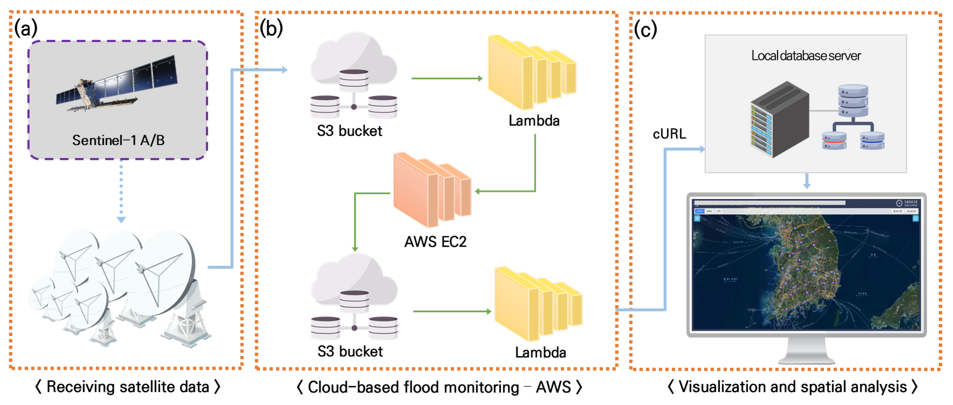
2.1. Overview of the Cloud-Based Flood Monitoring System Using Deep Learning with Land Cover Maps

For this research, a cloud-based flood monitoring system was developed as shown in Figure 1, which is fully automated, persistent, and operational. The processing chain of the deep learning-based system consists of three parts, including (a) receiving satellite data and preprocessing, (b) deep learning-based waterbody extraction through Amazon Web Services (AWS), and (c) visualization and spatial analysis.

For the fully automated flood monitoring system, the AWS cloud computing platform was adopted because the size of storage and memory provided by the platform is selectable, and the performance of the CPU and GPU is elastic and stable. The services are optimized to machine learning algorithms as computing resources are managed by automatically adjusting to the amount of required computation and the volume of input data. Newly acquired Sentinel-1 data, which are sensed and ingested regularly, is also directly available through the platform within a few hours as Sentinel-1 Ground Range Detected (GRD) products are regularly downloaded and added to the AWS S3 bucket through Copernicus OpenHub. At this stage, the data have already been converted to the cloud-optimized GeoTIFF format for deep learning-based image segmentation. For preprocessing and further analysis, the availability of satellite data is automatically checked every 10 min.

All of the necessary steps for near-real-time flood monitoring are programmed to automatically trigger next steps in turn in the platform. When the received Sentinel-1 data, which are available at the AWS open data bucket, are saved in Amazon Simple Storage Service (Amazon S3), event-based Lambda is automatically triggered to run the deep learning module for flooded area monitoring, by which the satellite data are segmented for waterbody extraction analysis. Satellite data are received and provided through its ground stations, and then the received Sentinel-1 data are immediately preprocessed using SNAP, which is provided by European Space Agency (ESA) for satellite data processing. SNAP is installed in the server and starts to run automatically by Lambda for satellite data preprocessing. In the Amazon Elastic Compute Cloud (Amazon EC2), the satellite data are stacked and cropped automatically for following image segmentation. It reduces time for reading and writing input data and output results.

The output results (e.g., segmented images) are transferred to a local database server via Client URL (cURL) for visualization and further spatial analysis. The procedure is completed with minimum time delay for publishing analysis results, which includes tiling of the output results for fast loading and visualization at various scales, taking a few minutes. Detailed explanation on deep learning-based image segmentation procedures in the cloud server is presented in the following section.

2.2. Deep Learning-Based Waterbody Extraction Using Land Cover Maps

In the cloud-based flood monitoring system shown in Figure 1, the deep learning-based waterbody extraction (i.e., part b in Figure 1) is the main step that determines the accuracy of image classification, and the usefulness of the flood monitoring system. The substeps of the step include preprocessing of satellite data, producing geospatial layers, and producing training data using land cover maps, and deep learning model training and inference, in addition to accuracy assessment (Figure 2). To realize and operationalize the substeps on the cloud platform, and to improve the accuracy of image segmentation using deep leaning, new algorithms were developed, and deep neural networks for image segmentation were customized and optimized in this research. Detailed explanation of the steps is presented in the following section.

3. Development of the Deep Learning-Based Waterbody Extraction Model

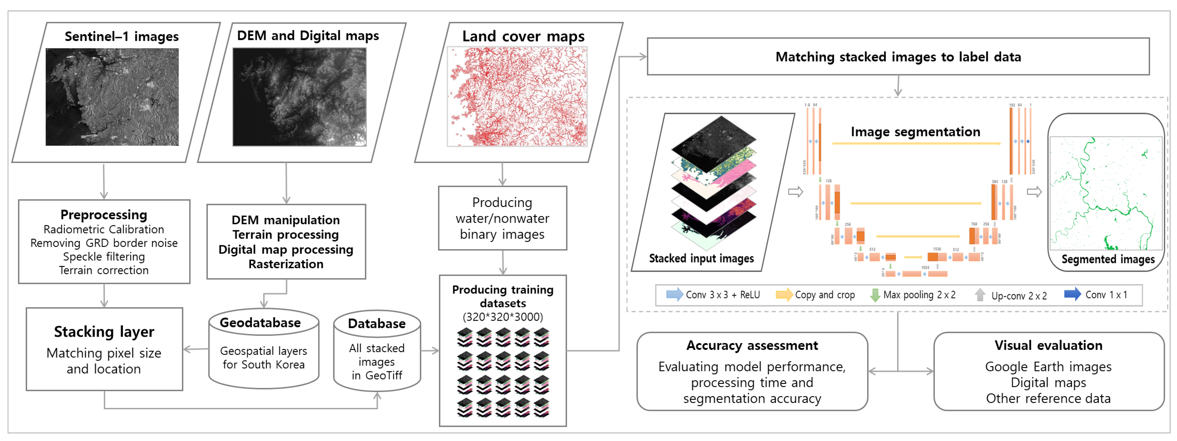
3.1. Producing Input Data

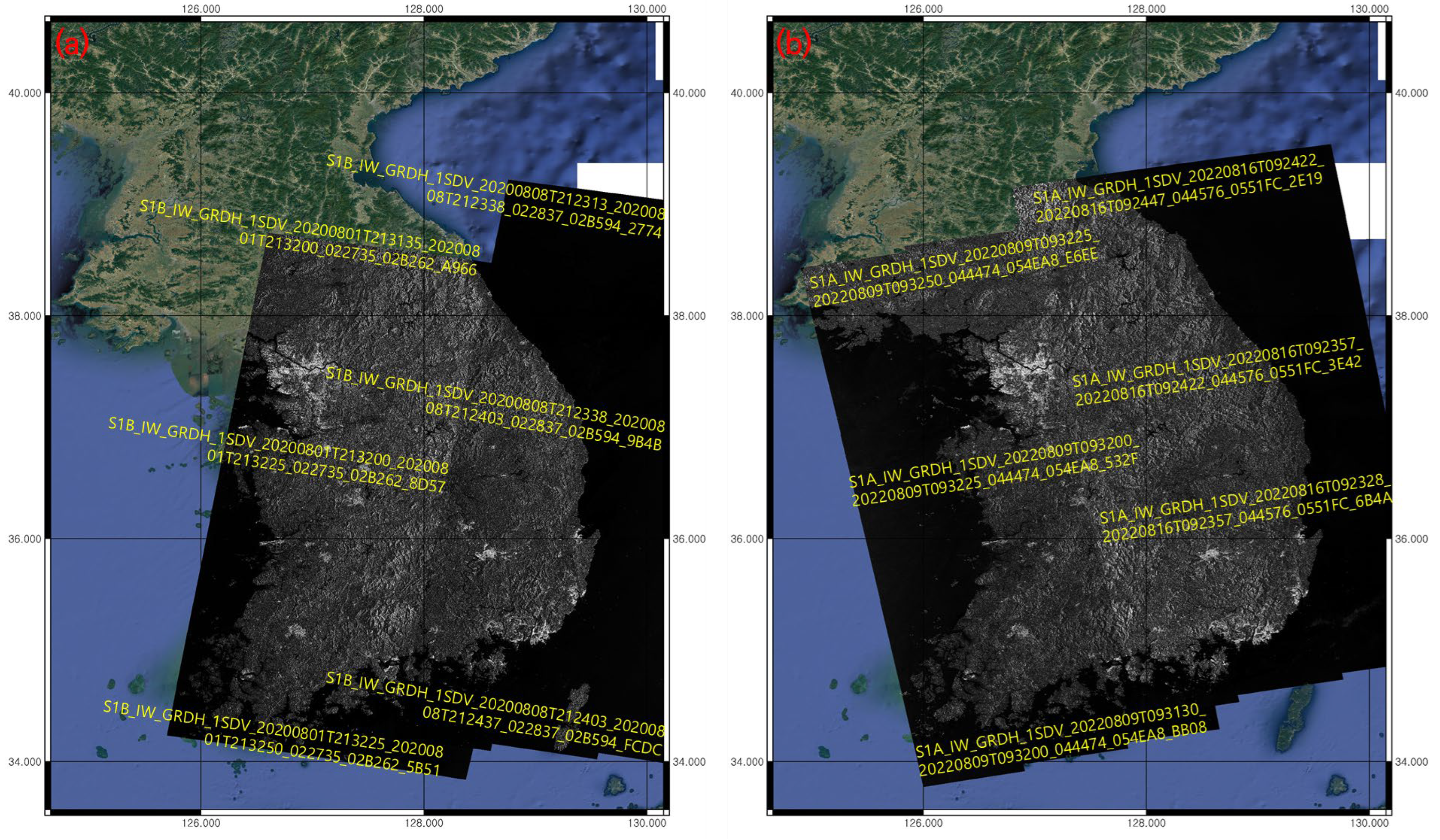
3.1.1. Preprocessing of Sentinel-1 Data and Producing Label Data

Two main input datasets for producing an initial deep leaning-based waterbody extraction model are Sentinel-1 images and land cover maps. To generate label data for deep learning model training and verification, detailed land cover maps of Republic of Korea were used, which were produced by the Ministry of Environment of Republic of Korea. The maps were produced using aerial photographs and satellite data including KOMPSAT-2, Landsat 7/8, and SPOT-5, after preprocessing and mosaicking of the satellite data. The accuracy of classification has been verified using reference data, such as digital maps, land registration maps, land use zoning maps, and forest-type maps, and through field survey. The final product maps, which have 41 land cover classes, are provided in shapefile format at 1:5000 scale. Of the classes, fresh water-related classes (i.e., rivers and lakes/reservoirs) were extracted and merged to produce label data, and verified through visual inspection for pixelwise class labeling (Figure 3a).

Sentinel-1 Ground Range Detected (GRD) images, which were obtained by a C-band Synthetic Aperture Radar (SAR) antenna launched by the European Space Agency (ESA), were downloaded from the Copernicus Open Access Hub (https://scihub.copernicus.eu/dhus/#/home, accessed on 15 February 2021), on the basis of locations and acquisition times that match those of the images for the detailed land cover maps. To generate input satellite images for flood monitoring, the original images were preprocessed through ‘Remove GRD border noise’, ‘Radiometric Calibration’, ‘Speckle Filtering’, and ‘Terrain Correction’ [33]. The preprocessed Sentinel-1 images, which are VV bands in linear scale at 10 m spatial resolution, were matched to the land cover maps for visual inspection (Figure 3b). After the inspection, the shapefiles (i.e., land cover maps) were converted to binary raster files to produce final label data (Figure 3c). The label data have two classes, i.e., water (0) and nonwater (1) in the GeoTiff file format, which have been rasterized to have the same spatial resolution with that of Sentinel-1 images.

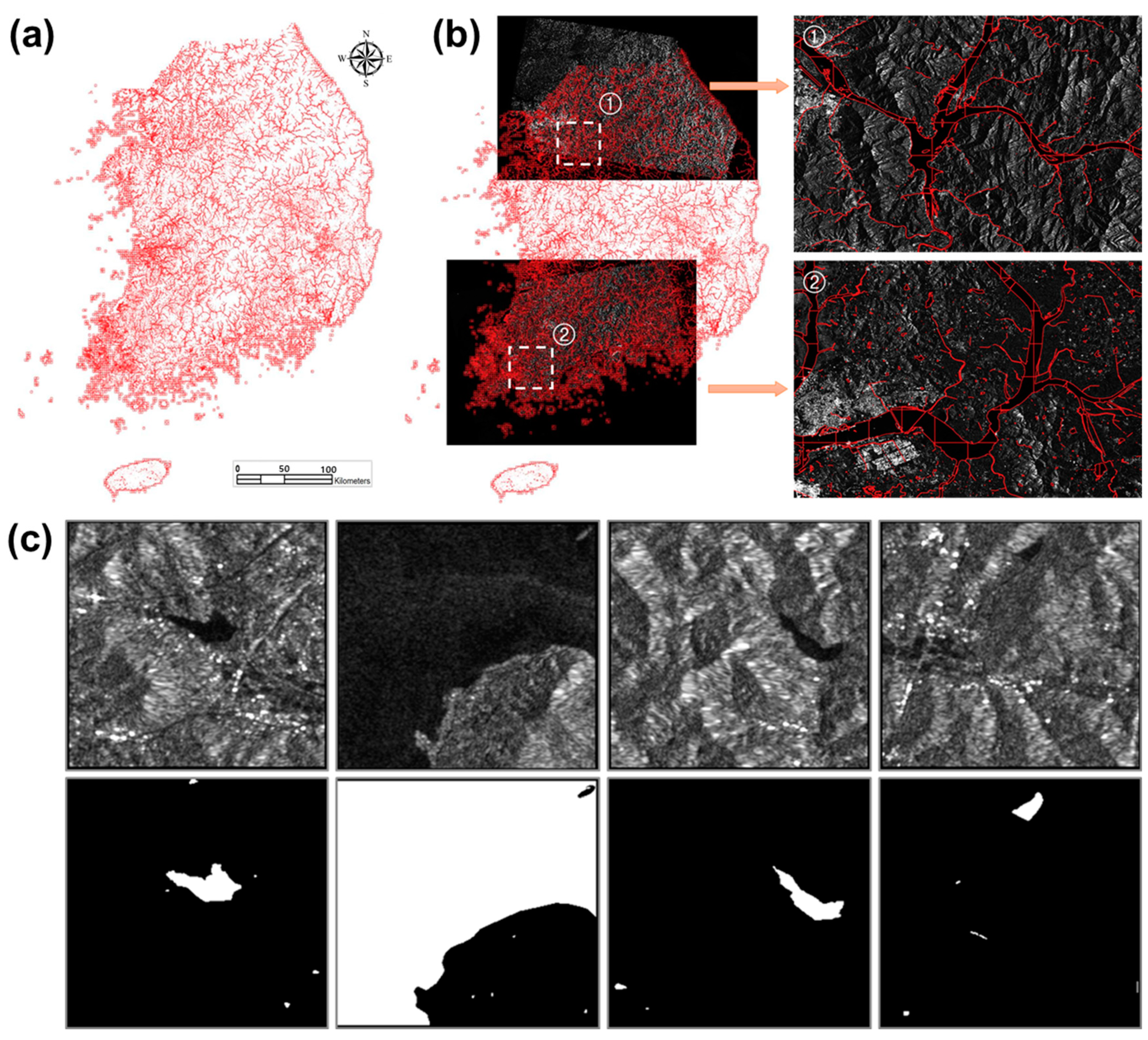
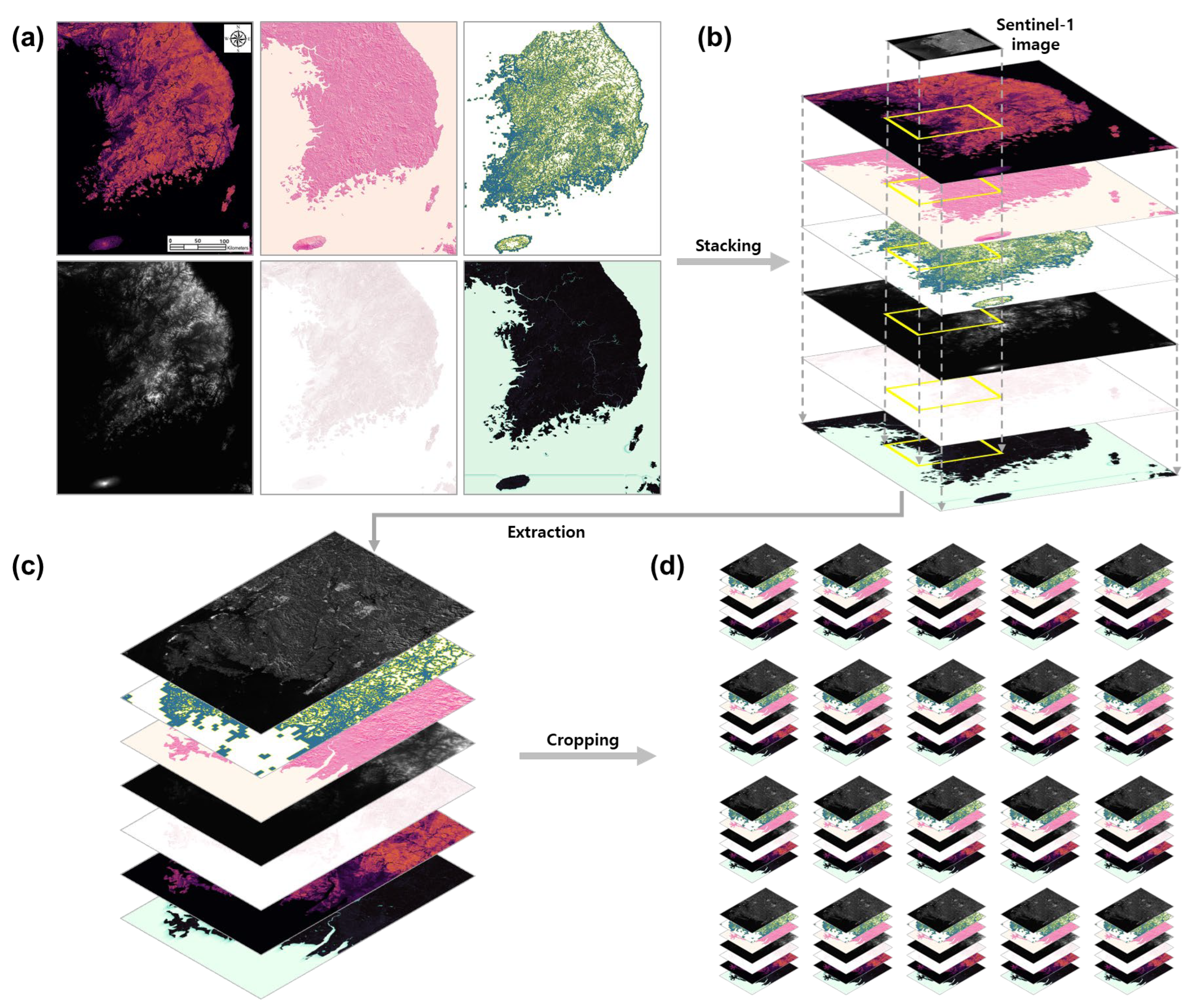
3.1.2. Producing Geospatial Layers and Stacking Input Layers

To improve the accuracy of deep learning-based image segmentation by combining geospatial data as input layers, seven geospatial layers were produced (Figure 4a). The layers include: (a) Digital Elevation Model (DEM) for Republic of Korea, (b) Terrain Ruggedness Index (TRI), (c) Topographic Wetness Index (TWI), (d) Profile Curvature (PC), (e) Aspect (AS), (f) Slope (SL), and (g) Buffer (BF). The layers were selected and produced in accordance with the principle and procedures presented in [34], which were expected to provide topohydrographic information during training and inference of the deep learning model. The geographical and spatial features contained in the layers improve the performance of classifying land cover classes and terrain effects as they represent the features of waterbodies and the surrounding environment, which are learned during the training of deep neural networks [34]. The DEM for Republic of Korea was mosaicked, inspected, and gap-filled for further processing, which has 10 m spatial resolution that matches with the spatial resolution of preprocessed Sentinel-1 images and label data. Using the DEM, the TRI, TWI, PC, AS, and SL inputs were produced based on the principles described in [35,36,37,38]. BF was produced using digital maps for Republic of Korea, which were produced in 2018 at 1:5000 scale. All the layers were produced and exported to a geospatial database in GeoTiff file format to determine the best combination of final input data and to optimize the deep learning model for automated flood monitoring.

All the input layers, including Sentinel-1 images, were overlaid and stacked by using the same spatial resolution and coordinate system, i.e., EPSG:4326 (WGS 84 latitude/longitude) coordinate, to be a multiband single image for model training. The values in the layers were normalized to have values between 0 and 1. The stacked images were extracted from the geospatial layers produced for the entire Republic of Korea region in accordance with the extent of Sentinel-1 images, and then the extracted layers were cropped out at the size optimal for model training. The procedures were conducted with new Python codes developed for this research. The size of the final image patches stacked for training was eight-layered 256 × 256 images, which was determined through repetitive experiments (Figure 4b–d), and the number of image patches produced for this research was 4110.

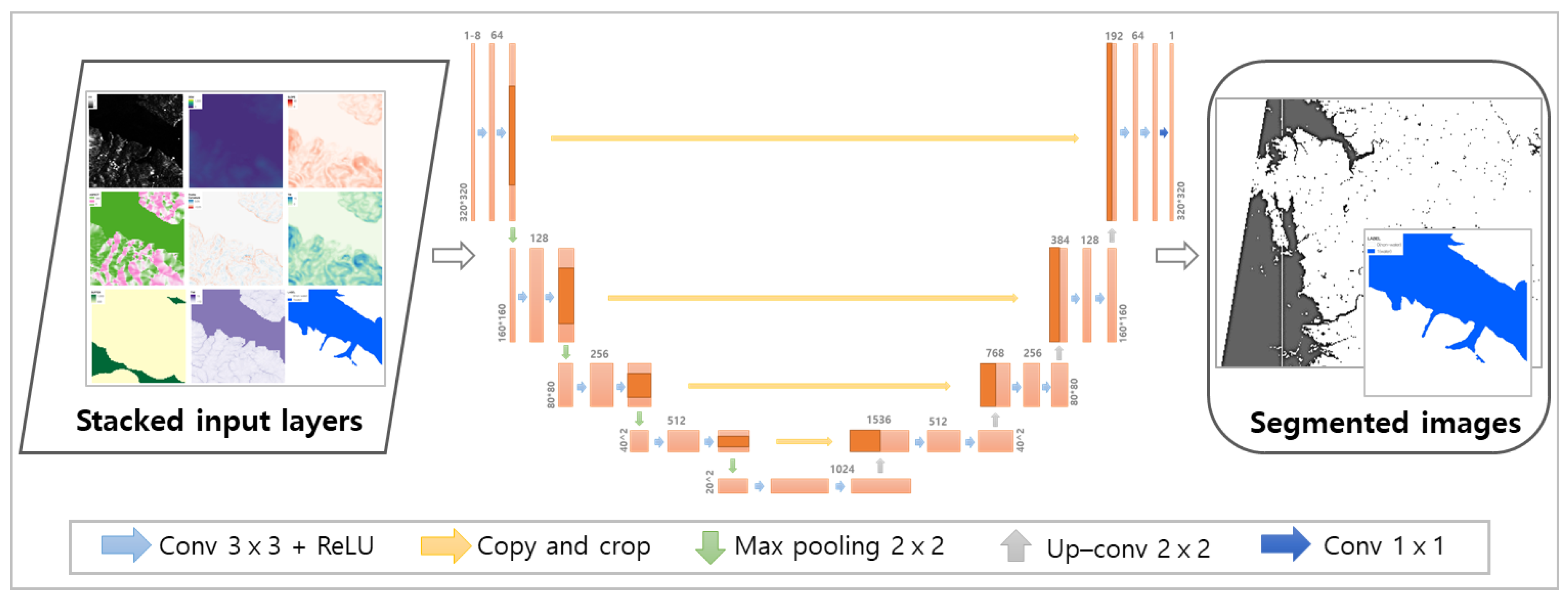
3.2. Developing Deep Learning-Based Image Segmentation Algorithm

3.2.1. Customization and Optimization of the Deep Neural Networks

For operational purposes, it is well known that the usefulness of outputs from satellite-based flood monitoring is often hampered by the spatial resolution of satellite data, and comparing to input satellite data, the spatial resolution of output feature maps become coarser due to convolution by kernel and downsampling with pooling layers in convolutional neural network (CNN)-based deep learning architectures, which are for extracting higher-level feature maps [39]. Considering such factors, pixel-based image segmentation was selected as the base of deep neural networks for the fully automated flood monitoring system to prevent losing spatial feature information contained in the original input data. To exploit the geospatial layers for improving image segmentation accuracy, the U-Net architecture was customized and optimized, which was presented by [40]. The architecture has shown good performance in semantic segmentation with minimum training data while retaining feature information of input data [41,42]. The deep neural network presented in this research was optimized for analyzing geolocated satellite and geospatial data, which were stacked as multilayered GeoTiff images.

As shown in Figure 5, the deep neural networks for multilayered image segmentation for this research extract higher-level feature maps with 18 3 × 3 2D convolution layers and four 2 × 2 2D max pooling layers during downsampling, and restore spatial resolution through four 2 × 2 upsampling layers in the expanding path and concatenation. Through the convolution and pooling layers, the deep neural network performs repeated downsampling and upsampling and interpolation to determine trainable parameters. Batch normalization layers are included in the deep learning architecture for image segmentation to exploit multilayered/big-sized data for wide areas. Through the customized and optimized network architecture, pixels and contextual information of input layers are learned for deep learning model generation and for waterbody extraction by image segmentation using the generated model.

3.2.2. Model Training and Inference

To derive the best deep learning model for this research, i.e., achieving best segmentation accuracy of satellite data using deep neural networks with highest spatial resolution and minimum processing time, we relied on both mathematical and empirical experiments. Using the training data produced for this research, the deep learning models were tested more than 500 times as preliminary analysis to test the effect of determining hyperparameters, spatial resolution of the dataset, optimal image patch size, water ratio, and the combination of input data layers. To evaluate the effectiveness of training, the training data were split into training, validation, and test datasets in the ratio of 3:1:1 [34]. Hyperparameters were tested and determined by repetitive experiments to achieve best segmentation accuracy with minimum loss (

Table 1. Hyperparameters for producing deep learning models for the flood monitoring system.

Hyperparameters for Producing Deep Learning Models
Kernel size (upsampling/output)	2 × 2/1 × 1
Stride/Padding	1 × 1/zero padding
Activation function	ReLU/sigmoid (output layer)
Learning rate/Decay rate	Adam optimizer 0.001/beta1 = 0.9, beta2 = 0.999
Max epoch/Iteration	1000/30 per epoch
Early stopping	No improvement of loss for ten epochs
Batch size	32
Patch size/Input channels	256 × 256/1–8
Training data/Water ratio	4110/0.1 and 0.3

), which was determined through focal Tversky loss. It was performed by changing input parameters in turn to identify best parameters of possible combinations using image patches of Sentinel-1 VV bands and corresponding label data. The kernel sizes of convolution layers were 2 × 2 and 1 × 1 for upsampling and output convolution layers, respectively, with a fixed stride of 1 × 1. RELU and sigmoid were used as the activation function for each layer and output layer, and zero padding was added to prevent losing spatial resolution of input data. Adam was employed as an optimizer, with a learning rate of 0.001 and decay rate set as 0.9 and 0.99 for beta1 and beta 2. For efficient training, input data were normalized through batch normalization with a batch size of 32, and maximum epoch was set as 1000 and iteration was 30 per epoch. Early stopping was used to minimize training time.

For inference, new satellite data were automatically matched and stacked with geospatial layers, and then cropped at the image size of 256 × 256 pixels. Inference was performed using trained models and parameters that were saved for image segmentation. After inference by image patches using trained models, the segmented image patches were mosaicked as a form of a georeferenced full-scene GeoTiff file for display, which is a 1 (water) and 2 (nonwater) valued binary image.

All the subprocesses for the fully automated flood monitoring, including preprocessing of satellite data and deep learning-based waterbody extraction, are operating with the AWS p2.xlarge instance that has four vCPUs, 61 GiB memory, and one Nvidia Telsa GPU, which has 12 Gb memories. The number of parallel processing cores is 2496, and network performance for the process is maintained as high.

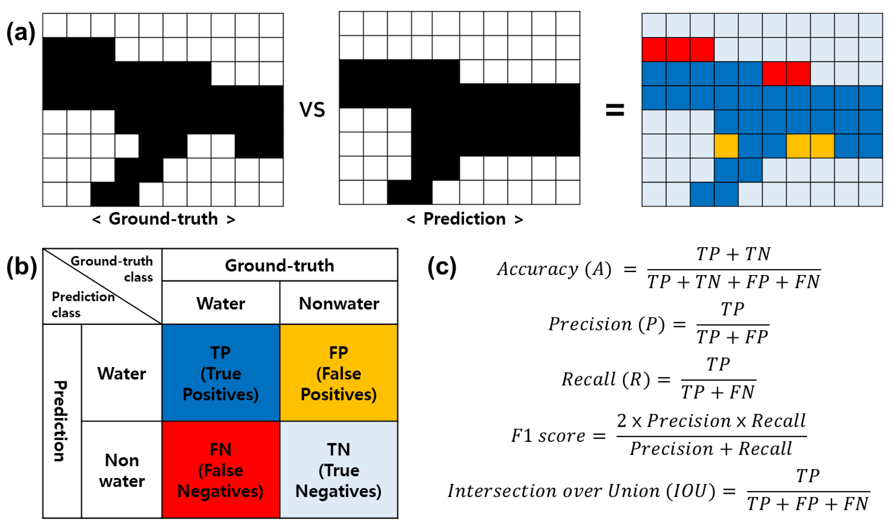
3.3. Evaluation of the Accuracy of Output Results

While the fully automated flood monitoring system operates regularly, the analysis results are evaluated for validating the quality of outputs. To evaluate the quality of output results, criteria for evaluating the accuracy of image segmentation have been applied to two flood events. The two cases are the major flood events that affected the entire territory of Republic of Korea, which occurred in August in 2020 and 2022. The cases can also demonstrate the operation of the fully automated flood monitoring system as the system operates automatically. For the flood events in 2020 and 2022, 12 Sentinel-1 images were downloaded as input data (Figure 6). Of the 12 images, the first six images in

Table 2. Selected Sentinel-1 images for evaluating deep learning-based image segmentation for the fully automated flood monitoring system.

No.	Satellite	Type/Mode	Acquisition Time (UTC)	Product ID	Usage
I-1	Sentinel-1A	GRDH/IW	2020/08/01 21:31:35–21:32:00	02B262_A966	Inference
I-2	Sentinel-1A	GRDH/IW	2020/08/01 21:32:00–21:32:25	02B262_8D57	Inference
I-3	Sentinel-1A	GRDH/IW	2020/08/01 21:32:25–21:32:50	02B262_5B51	Inference
I-4	Sentinel-1A	GRDH/IW	2020/08/08 21:23:13–21:23:38	02B594_2774	Inference
I-5	Sentinel-1A	GRDH/IW	2020/08/08 21:23:38–21:24:03	02B594_9B4B	Inference
I-6	Sentinel-1A	GRDH/IW	2020/08/08 21:24:03–21:24:37	02B594_FCDC	Inference
I-7	Sentinel-1B	GRDH/IW	2022/08/09 09:31:30–09:32:00	054EA8_BB08	Inference
I-8	Sentinel-1B	GRDH/IW	2022/08/09 09:32:00–09:32:25	054EA8_532F	Inference
I-9	Sentinel-1B	GRDH/IW	2022/08/09 09:32:25–09:32:50	054EA8_E6EE	Inference
I-10	Sentinel-1B	GRDH/IW	2022/08/16 09:23:28–09:23:57	0551FC_6B4A	Inference
I-11	Sentinel-1B	GRDH/IW	2022/08/16 09:23:57–09:24:22	0551FC_3E42	Inference
I-12	Sentinel-1B	GRDH/IW	2022/08/16 09:24:22–09:24:47	0551FC_2E19	Inference

are for the 2020 flood event (i.e., I-1 to I-6 in Table 2) and the other six images (i.e., I-7 to I-12 in Table 2) are for the 2022 flood events, which cover the entire Republic of Korea region.

The accuracy of deep learning-based image segmentation was evaluated in accordance with the confusion matrix and equations [43,44,45] shown in Figure 7. As training data were split into training, validation, and test datasets in the ratio of 3:1:1, validation and test datasets were used to evaluate training and inference accuracies in addition to model and system performance. Confusion matrices were produced by comparing actual vales of ground-truth data and predicted values of inferred images (Figure 7a,b). To evaluate model training, loss was estimated using validation datasets, in addition to producing confusion matrices. The validation was performed every 20 iterations to check the improvement of deep learning models by training. Using confusion matrices that were produced using test dataset, overall accuracy of pixelwise image segmentation, precision, recall, mean intersection over union (IOU), and F1 score were estimated through random sampling to evaluate image segmentation accuracy (Figure 7c).

4. Results

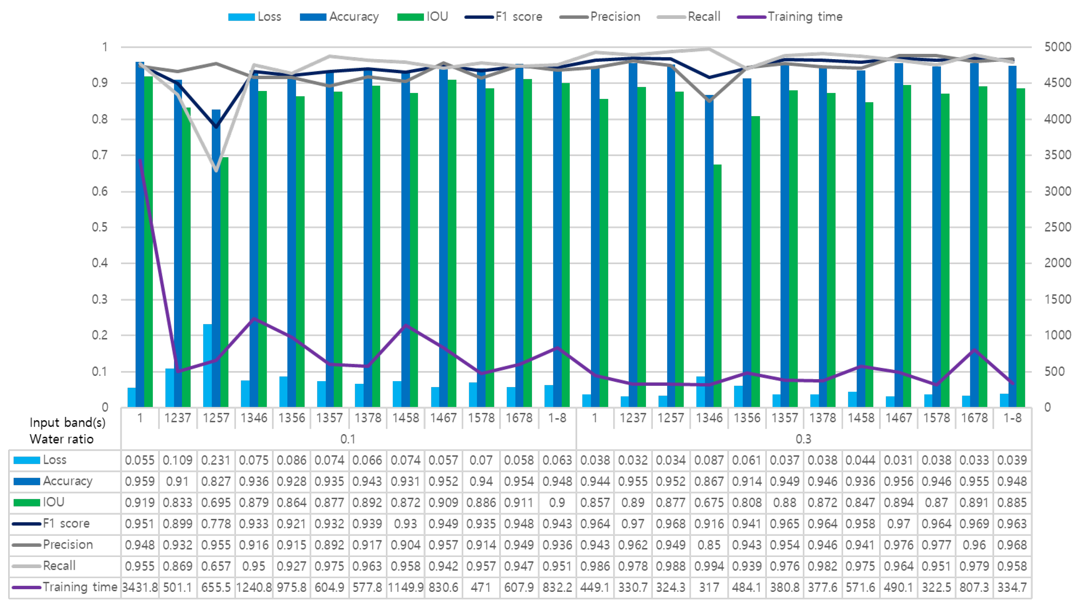
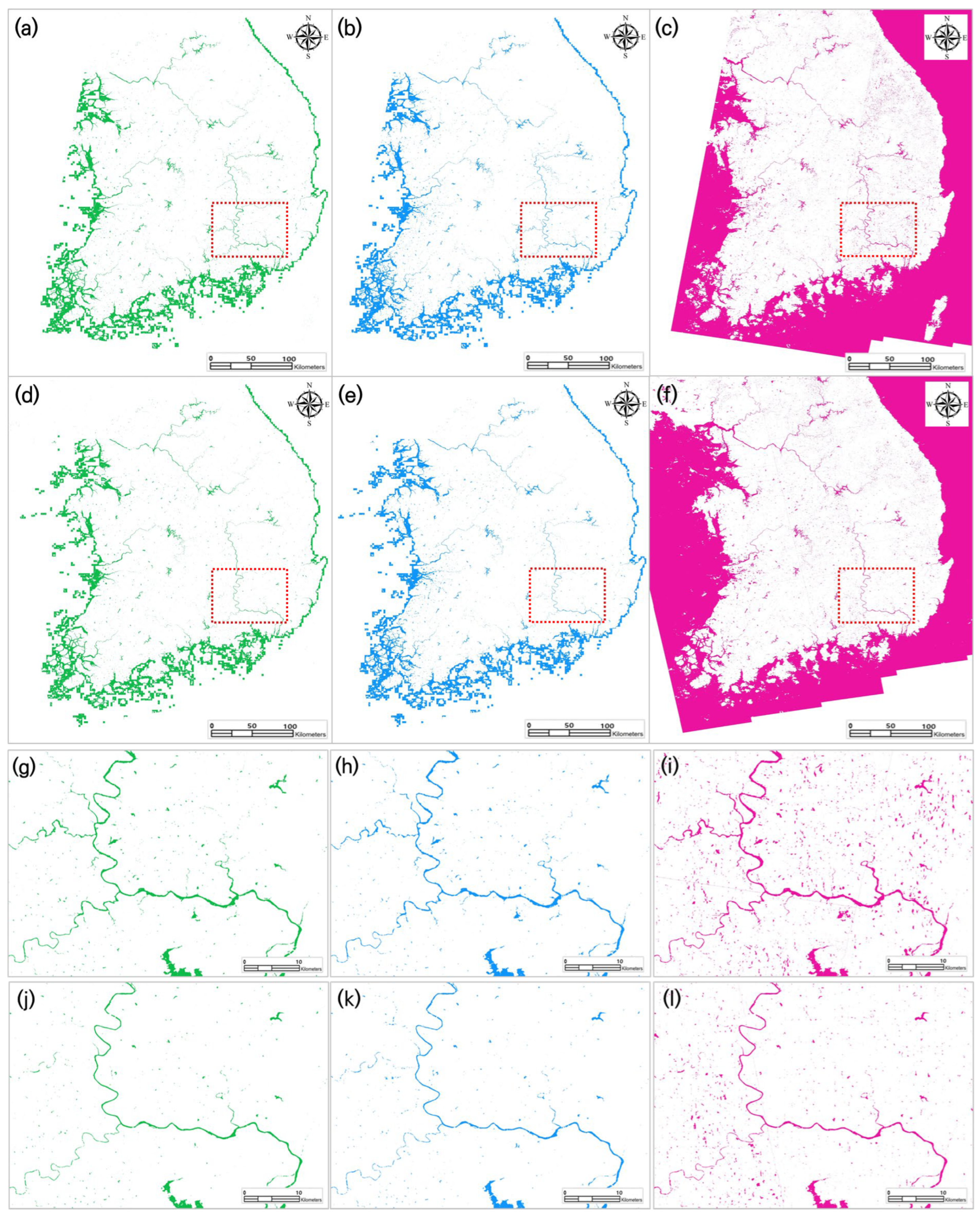
4.1. Image Segmentation by Waterbody Ratio

To develop the best deep learning model for fully automated flood monitoring, the accuracies of image segmentation were evaluated in accordance with the waterbody ratio of input image patches, after determining hyperparameters for training.

Table 3. Accuracy of image segmentation by waterbody ratio.

Water Ratio	No. of Patches	Training Time	Loss	Accuracy	Precision	Recall	IOU	F1 Score
5%	1038	512.1195 s	0.189	0.897	0.897	0.795	0.793	0.842
10%	745	705.3739 s	0.092	0.927	0.907	0.929	0.862	0.918
20%	511	418.7561 s	0.095	0.892	0.908	0.917	0.796	0.912
30%	370	373.3092 s	0.049	0.926	0.917	0.990	0.816	0.952

shows the results of estimated loss, overall accuracy, precision, recall, IOU, F1 score, and training time by waterbody ratio. The number of images patched for training decreased from 1038 to 370, as the waterbody ratio increased from 5% to 30%. The waterbody ratio 30% showed the lowest loss of 0.049 and highest F1 score of 0.952, whereas the waterbody ratio 10% showed the highest overall accuracy of 0.927 and IOU of 0.862. The waterbody ratio 30% also showed highest precision and recall, which were 0.917 and 0.990, respectively. Training time for 5%, 10%, 20%, and 30% of waterbody ratio were 512.1195, 705.3739, 418.7561, and 373.3092 s, respectively, showing the shortest training time for the 30% waterbody ratio.

4.2. Image Segmentation by Input Layers

In addition to the image segmentation by waterbody ratio of input image patches, the accuracies of image segmentation by different band combinations of the eight input bands were evaluated to present the best deep learning model for the fully automated flood monitoring system. The analysis results of more 300 tests on optimal band combinations show that some band combinations yielded higher precision, recall, and F1 score than those of the VV input bands. The band combinations also showed lower loss than the VV bands. The 30% waterbody ratio showed relatively higher segmentation accuracies and lower loss than those of the 10% waterbody ratio. The precision, overall accuracy, IOU, recall, and F1 score of ‘VV, AS, TWI, and BF input bands’ (1467-0.3 in Figure 8) were 0.976, 0.956, 0.894, 0.964, and 0.970, and those of ‘VV, DEM, SL, BF input bands’ (1237-0.3 in Figure 8) were 0.962, 0.955, 0.890, 0.978, and 0.970, whereas those of the VV input bands were 0.943, 0.944, 0.857, 0.986, and 0.964, respectively. Training time for this result was between 317.0 and 3431.8 s, showing that the training time for some band combinations was faster than that for the VV input bands.

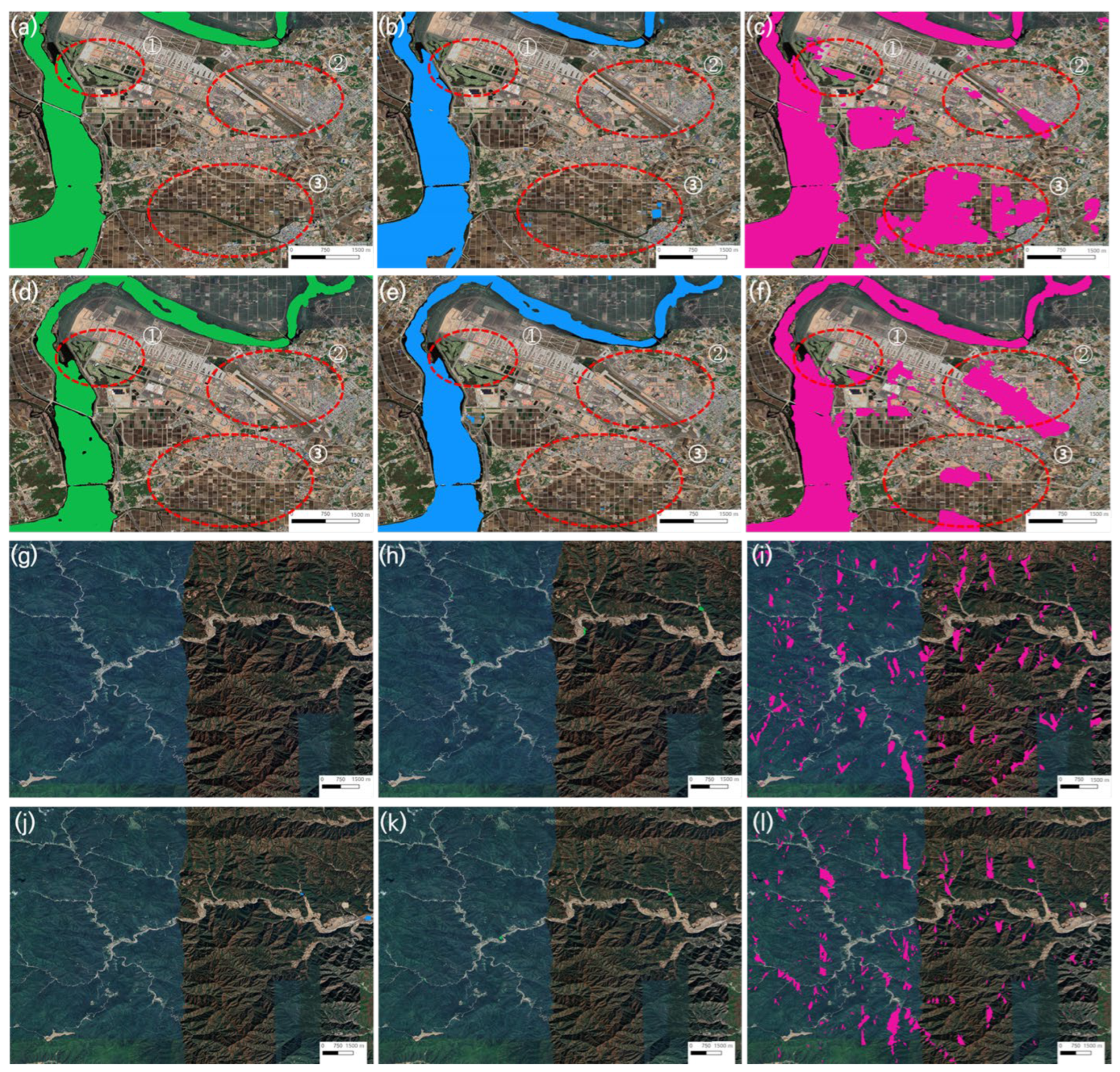
4.3. Image Segmentation for the Two Major Flood Events in 2020 and 2022

Using the deep learning models, which were produced by applying the testing procedures more than 500 times, 12 Sentinel-1 images for the entire Republic of Korea region were segmented in accordance with the hyperparameters presented in Table 1, waterbody ratio 30%, and different band combinations of the eight input bands. The automatically segmented Sentinel-1 images for the 2020 and 2022 flood events are presented in Figure 9, which are mosaicked results of six full-scene Sentinel images that cover the entire Republic of Korea region. Maps in Figure 9a–c show the output images for 2020 that were segmented using Figure 9a VV, AS, TWI, and BF input bands; Figure 9b VV, DEM, SL, BF input bands; and Figure 9c VV input band, while Figure 9d–f show segmented images for 2022 using Figure 9d VV, AS, TWI, BF input bands; Figure 9e VV, DEM, SL, BF input bands; and Figure 9f VV input band. Maps Figure 9g–l are enlarged images of the red boxes in Figure 9a–f, respectively, presented for visual comparison. As shown in Figure 9g–l, Figure 9c,f showed more misclassification than Figure 9a,b,de, which used four bands as input data, demonstrating the effectiveness of using geospatial layers in deep learning-based satellite image segmentation. This is explained in detail in the discussion section.

5. Discussion

5.1. Accuracy of Image Segmentation

The cloud-based flood monitoring system we developed advances the accuracy, frequency, and practicality of flood monitoring systems, or more generally waterbody extraction models that were presented by previous research. By presenting a customized deep neural network for satellite image segmentation, and by determining optimal hyperparameters, waterbody ratio, and band combination, the fully automated flood monitoring system showed 0.943, 0.944, 0.857, 0.986, and 0.964 of precision, overall accuracy, IOU, recall, and F1 score, when VV, AS, TWI, and BF input bands were used at 30% waterbody ratio for input training data. The results were verified by evaluating model performance and segmentation accuracy using the confusion matrix and equations explained in Section 3.3, which have been widely used in the remote sensing and computing science societies for evaluating the performance of deep learning-based image segmentation. The results demonstrate better, or comparable, performance of deep learning-based image segmentation for the fully automated flood monitoring system, compared to previous research. Fully automated waterbody extraction systems presented in [27,29] showed overall accuracies of 79 to 93% and 93%, respectively. Using thresholding-based classification for single-polarized data from Sentinel-1 images, [46] presented a fully automated processing chain for flood area mapping. The research showed overall accuracies between 94.0% and 96.1% and kappa coefficients between 0.879 and 0.910, but the experiment was confined to specific areas.

Based on intensive visual inspection, we assume that the improvement of segmentation accuracy is because of the effects of model training optimization procedures and geospatial layers. Misclassification of golf courses, airport runways, paddy fields, and terrain effects (such as mountain shadows) were extremely reduced, as shown in Figure 10. In SAR images, such constructed facilities and topographical features have been frequently misclassified due to the similarity of reflected signals [47]. During our experiments, it was also observed that objects in urban areas and paddy fields were sometimes misclassified, and we tried to minimize this misclassification through the procedures mentioned in the previous sections. Although we show segmentation accuracy was improved by the method presented in this research, the misclassification could not be completely removed because of the information contained in the input layers, which is still insufficient, and spatial and physical features of objects. Considering the assessment, the results of this research suggest that misclassification in SAR image classification or segmentation can be reduced by optimizing hyperparameters and training data, and employing the best combination of geospatial layers.

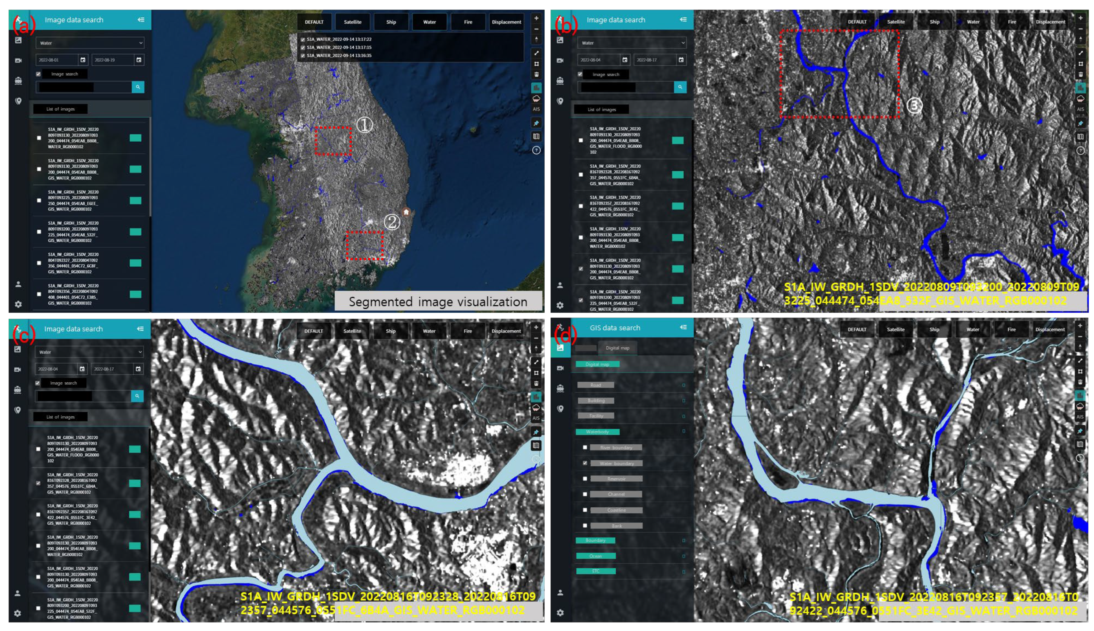
5.2. Processing Time, Memory Use, and Visualization

Once new satellite images are downloaded for flood monitoring, the images are automatically segmented using the optimal deep learning model installed in AWS. For image segmentation, only time for inference is needed for analyzing new satellite data, after preprocessing of the new satellite data. When one Nvidia Telsa GPU, which has 12 Gb memories, was used for inference, the time required for segmenting one full Sentinel-1 scene was between 648.5044 and 1144.7612 s (

Table 4. Inference time per scene by input band combinations.

Scene ID	Inference Time (Sec)
	VV AS TWI BF	VV DEM SL BF	VV
I-1 (02B262_A966)	854.4969	873.7666	857.9928
I-2 (02B262_8D57)	786.7988	795.0846	810.4651
I-3 (02B262_5B51)	695.3087	793.2391	751.3581
I-4 (02B594_2774)	871.7646	930.5432	905.7588
I-5 (02B594_9B4B)	744.1722	757.0344	762.0988
I-6 (02B594_FCDC)	724.4174	801.6264	807.6250
I-7 (054EA8_BB08)	711.2012	842.5217	839.9597
I-8 (054EA8_532F)	648.5044	827.2473	790.1158
I-9 (054EA8_E6EE)	678.2370	889.0405	830.3994
I-10 (0551FC_6B4A)	685.7259	916.4830	857.3961
I-11 (0551FC_3E42)	686.7059	896.8351	811.5082
I-12 (0551FC_2E19)	845.3665	1144.7612	1024.7044
Averaged time	744.3941	872.3501	837.4496

). As averaged inference time for the ‘VV, AS, TWI, and BF band combination’ was 744.3941 s, this was faster than the inference time of ‘VV bands’ or ‘VV, DEM, SL, and BF band combination’. For the inference and training of the deep neural network, around 11 Gb GPU memory was used out of 12 Gb, which is considered to be ‘not excessive’ and affordable for operating the fully automated flood monitoring system. As only one GPU is being used for inference, we think that the inference time is sufficient for rapid flood monitoring, and this is even faster than other fully automated image classification for rapid flood monitoring. The time for completing the processing chain presented by [46] was approximately 45 min for single-polarized data of a Sentinel-1 IW-GRD scene, which includes automatic thresholding, initial classification, and fuzzy logistic-based refinement. The approach proposed by [30] required 25 min for downloading satellite data, preprocessing, and inference. The time required for the same procedure in our system was approximately 15 min.

As explained in Section 2.1, after the analysis processes shown in the previous sections, the outputs produced on the cloud computing platform are sent to the local database server through cURL for visualization and further spatial analysis (Figure 11). The time required for visualization of outputs is negligible compared to the time for obtaining satellite data and image segmentation. The elastic cloud computing enabled stable analysis in part, reduced processing time, and shortened the time for obtaining satellite data. When river boundaries from digital maps (sky blue in Figure 11c,d) are overlaid on the segmentation outputs (blue in Figure 11a–d), the blue-colored areas outside the sky blue areas indicate flooded areas (see Figure 11c,d). Comparison between river boundaries and waterbody segmentation results is automatically performed without any human intervention to distinguish flooded areas. The visualization and spatial comparison provide information on flood situations at the time of satellite data acquisition, showing the operation of the fully automated flood monitoring system developed for this research. In this paper, although all available images are automatically downloaded and analyzed by the fully automated flood monitoring system, we present the segmentation results of 12 Sentinel-1 images in Figure 6 as examples. It was observed that all of the outputs of the fully automated flood monitoring system show similar segmentation accuracy, processing time, and stable performance, demonstrating robustness of the method presented in this research for flood monitoring.

5.3. Novelty and Contribution

As aforementioned, fully automated flood monitoring has been limited by developing processing systems, the accuracy of satellite image segmentation, and processing time, in addition to the operationalization of the automated processing systems. This is not the first research that presents a fully automated flood monitoring system, but we think that this research advances actual satellite-based flood monitoring practices and existing studies by demonstrating the fact that such practices can be achieved by presenting optimally trained deep learning models, cloud-based computing, and training data generation using land cover maps. The results of this research show that the improved accuracy and processing time of satellite image segmentation meet the need for practical flood monitoring, as shown in the previous sections. We think, therefore, that the results of this research and the flood monitoring system presented in this study provide both academic and technological advancement. To improve the accuracy of flood area extraction using deep learning, reduce processing time, and operationalize the fully automated flood monitoring, this research focused rather on optimization and customization of an existing deep learning architecture and hyperparameters for input data through intensive experiments, producing high-quality input datasets for training and inference, and adopting and linking cloud-based computing, rather than focusing on presenting new deep learning networks. As this research provides a technological contribution, in addition to its academic contribution, the results of this research can be used as a benchmark for building an operational flood monitoring system for rapid and stable flood monitoring using deep learning with higher image classification accuracy and faster processing time.

5.4. Implication, Limitations, and Future Work

The implication of this research lies not only in satellite image segmentation for flood monitoring and building a fully automated flood monitoring system, but also deep learning-based satellite image classification for other purposes and building satellite-based disaster monitoring systems. The findings of this research suggest that deep learning-based flood monitoring using satellite data can achieve higher image segmentation accuracy, compared to existing previous studies, and the fully automated flood monitoring system developed through this research can be operationalized for practical purposes.

However, by developing a processing chain for persistent flood monitoring using cloud computing and intensive tests of hyperparameters, waterbody ratio, and band combinations for flood area extraction, from which a fully automated flood monitoring system is presented in this research, the usability of the findings of this research need to be demonstrated for other regions. The results of this research showed higher image segmentation accuracy and processing time for flood monitoring, but they were developed and tested for the Republic of Korea region. Although the flood monitoring system presented in this research can be implemented for both rural and urban areas, the development of the system is focused more on monitoring floods in rural areas and during rainy seasons; these areas are more frequently affected by river floods than flush floods in urban areas due to the flood drainage system. For urban areas in Republic of Korea, there are other means for flood monitoring, for example CCTV, but such means and accessibility are limited in rural areas. In addition, as the flood monitoring system presented in this research focuses on estimating the extent of floods by exploiting Sentinel-1 data, the magnitude of floods that includes velocity and depth of water need to be evaluated by combining other ancillary data. To enhance the frequency, spatial resolution, and accuracy of flood monitoring, the possibility of adapting other satellite data, such as ICEYE and Spacety SAR constellations, to the system needs to be tested.

6. Conclusions

Developing a fully automated flood monitoring system using satellite data has been limited by present processing systems, processing time and accuracy of image segmentation, and the operationalization of the automated processing system. To overcome these obstacles, a deep learning-based flood area extraction model for a fully automated flood monitoring system is presented in this research, which is designed to operate persistently on a cloud-based computing platform. The system regularly extracts flooded areas from Sentinel-1 data, and thus provides visual information on flood situations. As the results of this research showed that deep learning-based flood monitoring using satellite data can achieve higher image segmentation accuracy, and the fully automated flood monitoring system developed through this research can be operationalized for practical purposes, the system was presented by developing a processing chain for persistent flood monitoring using cloud computing, and presenting optimal deep learning models and input data. Intensive tests of hyperparameters, waterbody ratio, and band combinations for flood area extraction were conducted to improve image segmentation accuracy. Since this research showed improved accuracy for flood area extraction using deep learning, reduced processing time, and operationalization of a fully automated flood monitoring system, the results of this research can be a reference to satellite image segmentation for flood monitoring, building a fully automated flood monitoring system, and deep learning-based satellite image classification for other purposes, such as building satellite-based disaster monitoring systems.

References

1. Mikkelsen, P.S.; Adeler, O.F.; Albrechtsen, H.J.; Henze, M. Collected Rainfall as a Water Source in Danish Households–What Is the Potential and What Are the Costs? Water Sci. Technol. 1999, 39, 49–56. [Google Scholar] [CrossRef]
2. Westra, S.; Fowler, H.J.; Evans, J.P.; Alexander, L.V.; Berg, P.; Johnson, F.; Kendon, E.J.; Lenderink, G.; Roberts, N. Future Changes to the Intensity and Frequency of Short-duration Extreme Rainfall. Rev. Geophys. 2014, 52, 522–555. [Google Scholar] [CrossRef] [Green Version]
3. Matgen, P.; Martinis, S.; Wagner, W.; Freeman, V.; Zeil, P.; McCormick, N. Feasibility Assessment of an Automated, Global, Satellite-Based Flood-Monitoring Product for the Copernicus Emergency Management Service; EUR 30073 EN; Publications Office of the European Union: Luxembourg, 2020; pp. 1–47. ISBN 978-92-76-10254-0. [Google Scholar] [CrossRef]
4. Ives, J.D.; Messerli, B. Mountain Hazards Mapping in Nepal Introduction to an Applied Mountain Research Project. Mt. Res. Dev. 1981, 1, 223–230. [Google Scholar] [CrossRef]
5. Rimal, B.; Zhang, L.; Keshtkar, H.; Sun, X.; Rijal, S. Quantifying the Spatiotemporal Pattern of Urban Expansion and Hazard and Risk Area Identification in the Kaski District of Nepal. Land 2018, 7, 37. [Google Scholar] [CrossRef] [Green Version]
6. Munawar, H.S. Flood Disaster Management: Risks, Technologies, and Future Directions. Mach. Vis. Insp. Syst. Image Process. Concepts Methodol. Appl. 2020, 1, 115–146. [Google Scholar]
7. Cao, S.; Zheng, H. Climate Change Adaptation to Escape the Poverty Trap: Role of the Private Sector. Ecosyst. Health Sustain. 2016, 2, e01244. [Google Scholar] [CrossRef] [Green Version]
8. Sharma, T.P.P.; Zhang, J.; Koju, U.A.; Zhang, S.; Bai, Y.; Suwal, M.K. Review of Flood Disaster Studies in Nepal: A Remote Sensing Perspective. Int. J. Disaster Risk Reduct. 2019, 34, 18–27. [Google Scholar] [CrossRef]
9. Kundzewicz, Z.W.; Kanae, S.; Seneviratne, S.I.; Handmer, J.; Nicholls, N.; Peduzzi, P.; Mechler, R.; Bouwer, L.M.; Arnell, N.; Mach, K.; et al. Flood Risk and Climate Change: Global and Regional Perspectives. Hydrol. Sci. J. 2013, 59, 1–28. [Google Scholar] [CrossRef] [Green Version]
10. Komori, D.; Nakamura, S.; Kiguchi, M.; Nishijima, A.; Yamazaki, D.; Suzuki, S.; Kawasaki, A.; Oki, K.; Oki, T. Characteristics of the 2011 Chao Phraya River flood in Central Thailand. Hydrol. Res. Lett. 2012, 6, 41–46. [Google Scholar] [CrossRef]
11. Kundu, S.; Aggarwal, S.P.; Kingma, N.; Mondal, A.; Khare, D. Flood Monitoring Using Microwave Remote Sensing in a Part of Nuna River Basin, Odisha, India. Nat. Hazards 2015, 76, 123–138. [Google Scholar] [CrossRef]
12. Bilali, A.E.; Taleb, I.; Nafii, A.; Taleb, A. A practical probabilistic approach for simulating life loss in an urban area associated with a dam-break flood. Int. J. Disaster Risk Reduct. 2022, 76, 103011. [Google Scholar] [CrossRef]
13. Zhuo, L.; Han, D. Agent-based modelling and flood risk management: A compendious literature review. J. Hydrol. 2020, 591, 125600. [Google Scholar] [CrossRef]
14. Long, S.; Fatoyinbo, T.E.; Policelli, F. Flood Extent Mapping for Namibia Using Change Detection and Thresholding with SAR. Environ. Res. Lett. 2014, 9, 035002. [Google Scholar] [CrossRef]
15. Rahman, M.R.; Thakur, P.K. Detecting, Mapping and Analysing of Flood Water Propagation Using Synthetic Aperture Radar (SAR) Satellite Data and GIS: A Case Study from the Kendrapara District of Orissa State of India. Egypt. J. Remote. Sens. Space Sci. 2018, 21, S37–S41. [Google Scholar] [CrossRef]
16. Tsyganskaya, V.; Martinis, S.; Marzahn, P.; Ludwig, R. SAR-based Detection of Flooded Vegetation–a Review of Characteristics and Approaches. Int. J. Remote Sens. 2018, 39, 2255–2293. [Google Scholar] [CrossRef]
17. Shen, X.; Wang, D.; Mao, K.; Anagnostou, E.; Hong, Y. Inundation Extent Mapping by Synthetic Aperture Radar: A Review. Remote Sens. 2019, 11, 879. [Google Scholar] [CrossRef] [Green Version]
18. Bauer-Marschallinger, B.; Cao, S.; Navacchi, C.; Freeman, V.; Reuß, F.; Geudtner, D.; Rommen, B.; Vega, F.C.; Snoeij, P.; Attema, E.; et al. The Normalised Sentinel-1 Global Backscatter Model, Mapping Earth’s Land Surface with C-band Microwaves. Sci. Data 2021, 8, 277. [Google Scholar] [CrossRef]
19. Matgen, P.; Hostache, R.; Schumann, G.; Pfister, L.; Hoffmann, L.; Savenije, H.H.G. Towards an Automated SAR-based Flood Monitoring System: Lessons Learned from Two Case Studies. Phys. Chem. Earth, Parts A/B/C 2011, 36, 241–252. [Google Scholar] [CrossRef]
20. Lu, J.; Giustarini, L.; Xiong, B.; Zhao, L.; Jiang, Y.; Kuang, G. Automated Flood Detection with Improved Robustness and Efficiency Using Multi-temporal SAR Data. Remote Sens. Lett. 2014, 5, 240–248. [Google Scholar] [CrossRef]
21. Martinis, S.; Kersten, J.; Twele, A. A Fully Automated TerraSAR-X based Flood Service. ISPRS J. Photogramm. Remote Sens. 2015, 104, 203–212. [Google Scholar] [CrossRef]
22. Cian, F.; Marconcini, M.; Ceccato, P. Normalized Difference Flood Index for Rapid Flood Mapping: Taking Advantage of EO Big Data. Remote Sens. Environ. 2018, 209, 712–730. [Google Scholar] [CrossRef]
23. Cerrai, D.; Yang, Q.; Shen, X.; Koukoula, M.; Anagnostou, E.N. Brief communication: Hurricane Dorian: Automated Near-real-time Mapping of the “Unprecedented” Flooding in the Bahamas Using Synthetic Aperture Radar. Nat. Hazards Earth Syst. Sci. 2020, 20, 1463–1468. [Google Scholar] [CrossRef]
24. Martinis, S.; Twele, A.; Voigt, S. Towards Operational Near Real-time Flood Detection Using a Split-based Automatic Thresholding Procedure on High Resolution TerraSAR-X Data. Nat. Hazards Earth Syst. Sci. 2009, 9, 303–314. [Google Scholar] [CrossRef]
25. Chini, M.; Hostache, R.; Giustarini, L.; Matgen, P. A Hierarchical Split-based Approach for Parametric Thresholding of SAR Images: Flood Inundation as a Test Case. IEEE T. Geosci. Remote Sens. 2017, 55, 6975–6988. [Google Scholar] [CrossRef]
26. Giustarini, L.; Hostache, R.; Matgen, P.; Schumann, G.J.P.; Bates, P.D.; Mason, D.C. A Change Detection Approach to Flood Mapping in Urban Areas Using TerraSAR-X. IEEE T. Geosci. Remote Sens. 2012, 51, 2417–2430. [Google Scholar] [CrossRef] [Green Version]
27. Huang, W.; DeVries, B.; Huang, C.; Lang, M.W.; Jones, J.W.; Creed, I.F.; Carroll, M.L. Automated Extraction of Surface Water Extent from Sentinel-1 Data. Remote Sens. 2018, 10, 797. [Google Scholar] [CrossRef] [Green Version]
28. Ireland, G.; Volpi, M.; Petropoulos, G.P. Examining the Capability of Supervised Machine Learning Cassifiers in Extracting Flooded Areas from Landsat TM Imagery: A Case Study from a Mediterranean Flood. Remote Sens. 2015, 7, 3372–3399. [Google Scholar] [CrossRef] [Green Version]
29. Shen, X.; Anagnostou, E.N.; Allen, G.H.; Brakenridge, G.R.; Kettner, A.J. Near-real-time Non-obstructed Flood Inundation Mapping Using Synthetic Aperture Radar. Remote Sens. Environ. 2019, 221, 302–315. [Google Scholar] [CrossRef]
30. Nemni, E.; Bullock, J.; Belabbes, S.; Bromley, L. Fully Convolutional Neural Network for Rapid Flood Segmentation in Synthetic Aperture Radar Imagery. Remote Sens. 2020, 12, 2532. [Google Scholar] [CrossRef]
31. Kang, W.; Xiang, Y.; Wang, F.; Wan, L.; You, H. Flood Detection in Gaofen-3 SAR Images via Fully Convolutional Networks. Sensors 2018, 18, 2915. [Google Scholar] [CrossRef]
32. Zhu, X.X.; Tuia, D.; Mou, L.; Xia, G.S.; Zhang, L.; Xu, F.; Fraundorfer, F. Deep Learning in Remote Sensing: A Comprehensive Review and List of Resources. IEEE Geosci. Remote Sens. Mag. 2017, 5, 8–36. [Google Scholar] [CrossRef] [Green Version]
33. Scarpa, G.; Gargiulo, M.; Mazza, A.; Gaetano, R. A CNN-based Fusion Method for Feature Extraction from Sentinel Data. Remote Sens. 2018, 10, 236. [Google Scholar] [CrossRef] [Green Version]
34. Kim, J.; Kim, H.; Jeon, H.; Jeong, S.H.; Song, J.; Vadivel, S.K.P.; Kim, D.J. Synergistic Use of Geospatial Data for Water Body Extraction from Sentinel-1 Images for Operational Flood Monitoring across Southeast Asia Using Deep Neural Networks. Remote Sens. 2021, 13, 4759. [Google Scholar] [CrossRef]
35. Beven, K.J.; Kirkby, M.J. A Physically Based, Variable Contributing Area Model of Basin Hydrology. Hydrol. Sci. J. 1979, 24, 43–69. [Google Scholar] [CrossRef] [Green Version]
36. Tarboton, D.G. A New Method for the Determination of Flow Directions and Upslope Areas in Grid Digital Elevation Models. Water Resour. Res. 1997, 33, 309–319. [Google Scholar] [CrossRef] [Green Version]
37. Riley, S.J.; DeGloria, S.D.; Elliot, R. Index that Quantifies Topographic Heterogeneity. Intermt. J. Sci. 1999, 5, 23–27. [Google Scholar]
38. Sörensen, R.; Zinko, U.; Seibert, J. On the Calculation of the Topographic Wetness Index: Evaluation of Different Methods Based on Field Observations. Hydrol. Earth Syst. Sci. 2006, 10, 101–112. [Google Scholar] [CrossRef] [Green Version]
39. Bentivoglio, R.; Isufi, E.; Jonkman, S.N.; Taormina, R. Deep Learning Methods for Flood Mapping: A Review of Existing Applications and Future Research Directions. Hydrol. Earth Syst. Sci. 2022, 26, 4345–4378. [Google Scholar] [CrossRef]
40. Ronneberger, O.; Fischer, P.; Brox, T. U-net: Convolutional Networks for Biomedical Image Segmentation. In Proceedings of the International Conference on Medical Image Computing and Computer-Assisted Intervention, Munich, Germany, 5–9 October 2015; pp. 234–241. [Google Scholar]
41. Du, L.; McCarty, G.W.; Zhang, X.; Lang, M.W.; Vanderhoof, M.K.; Li, X.; Huang, C.; Lee, S.; Zou, Z. Mapping Forested Wetland Inundation in the Delmarva Peninsula, USA Using Deep Convolutional Neural Networks. Remote Sens. 2020, 12, 644. [Google Scholar] [CrossRef] [Green Version]
42. Wang, S.; Chen, W.; Xie, S.M.; Azzari, G.; Lobell, D.B. Weakly Supervised Deep Learning for Segmentation of Remote Sensing Imagery. Remote Sens. 2020, 12, 207. [Google Scholar] [CrossRef] [Green Version]
43. Zhang, P.; Gong, M.; Su, L.; Liu, J.; Li, Z. Change Detection Based on Deep Feature Representation and Mapping Transformation for Multi-spatial-resolution Remote Sensing Images. ISPRS J. Photogramm. Remote Sens. 2016, 116, 24–41. [Google Scholar] [CrossRef]
44. Buscombe, D.; Ritchie, A.C. Landscape Classification with Deep Neural Networks. Geosciences 2018, 8, 244. [Google Scholar] [CrossRef] [Green Version]
45. Ouled Sghaier, M.; Hammami, I.; Foucher, S.; Lepage, R. Flood Extent Mapping from Time-series SAR Images Based on Texture Analysis and Data Fusion. Remote Sens. 2018, 10, 237. [Google Scholar] [CrossRef] [Green Version]
46. Twele, A.; Cao, W.; Plank, S.; Martinis, S. Sentinel-1-based Flood Mapping: A Fully Automated Processing Chain. Int. J. Remote Sens. 2016, 37, 2990–3004. [Google Scholar] [CrossRef]
47. Manavalan, R. SAR Image Analysis Techniques for Flood Area Mapping-literature Survey. Earth Sci. Inform. 2017, 10, 1–14. [Google Scholar] [CrossRef]
Figure 1. Processing chain for fully automated waterbody extraction for regular flood monitoring: (a) receiving satellite data, (b) deep learning-based flood area extraction on Amazon Web Services (AWS), and (c) visualization and spatial analysis.
Remotesensing 14 06373 g001
Figure 2. Algorithm of the deep learning-based waterbody extraction in this research (These steps include preprocessing of satellite data, producing geospatial layers, and producing training data using land cover maps, deep learning model training and inference, and accuracy assessment.).
Remotesensing 14 06373 g002
Figure 3. Producing training data for the research: (a) mosaicked land cover maps for 2018; (b) land cover maps overlaid on Sentinel-1 images for matching and cropping layers, and enlarged images ① and ② for visual verification; (c) examples of paired satellite image patches (top) and label data (bottom) produced for training and inference.
Remotesensing 14 06373 g003
Figure 4. Geospatial layers produced for this research and stacking and cropping input layers: (a) produced geospatial layers for Republic of Korea, (b) stacked geospatial layers, (c) extracting stacked layers (around 30,000 × 20,000 pixels), and (d) cropping the stacked layers for deep learning model training (256 × 256 × 8 bands).
Remotesensing 14 06373 g004
Figure 5. Architecture of the optimized deep neural network for multilayered input image segmentation.
Remotesensing 14 06373 g005
Figure 6. Sentinel-1 images for the two major flood events in August in (a) 2020 and (b) 2022.
Remotesensing 14 06373 g006
Figure 7. Accuracy assessment of image-segmented output images: (a) ground-truth data and prediction result for comparison; (b) confusion matrix for accuracy assessment; and (c) equations for evaluating accuracy, precision, recall, F1 score, and IOU.
Remotesensing 14 06373 g007
Figure 8. Accuracy of image segmentation by water ratio and combinations of input layers (numbers in the input band(s) column indicate band combinations of 1-VV, 2-DEM, 3-SL, 4-AS, 5-PC, 6-TWI, 7-BF, and 8-TRI).
Remotesensing 14 06373 g008
Figure 9. Automatically segmented Sentinel-1 images for 2020 and 2022: (a) VV, AS, TWI, BF combination for 2020; (b) VV, DEM, SL, BF combination for 2020; (c) VV for 2020; (d) VV, AS, TWI, BF combination for 2022; (e) VV, DEM, SL, BF combination for 2022; (f) VV for 2022; and (gl) are zoom-in images of the red boxes shown in (af), respectively.
Remotesensing 14 06373 g009
Figure 10. Segmentation results overlaid on Google Earth images ((ac,gi) are for 2020, (df,jl) are for 2022; first column—VV, AS, TWI, BF combination, second column—VV, DEM, SL, BF, combination, and third column—VV images; first and second rows ① to ③ show differences in segmentation results for airport runways, golf courses, and paddy fields, respectively, and the third and fourth rows show differences in segmentation results for mountain shadows.
Remotesensing 14 06373 g010
Figure 11. Visualization and spatial analysis of output images: (a) visualization of fully automated flood monitoring for the 2022 flood event, (b) enlarged image of ① in (a)—automatically extracted waterbodies; (c) enlarged image of ② in (a)—river boundaries from digital maps (sky blue) overlaid on extracted waterbodies; (d) enlarged image of ③—blue color shows flooded areas.
Remotesensing 14 06373 g011