Article

Detecting Spatially Non-Stationary between Vegetation and Related Factors in the Yellow River Basin from 1986 to 2021 Using Multiscale Geographically Weighted Regression Based on Landsat

1
The School of Geoscience and Technology, Zhengzhou University, Zhengzhou 450052, China
2
Joint Laboratory of Eco-Meteorology, Chinese Academy of Meteorological Sciences, Zhengzhou University, Zhengzhou 450052, China
3
National Engineering Research Center for Geographic Information System, School of Geography and Infor-mation Engineering, China University of Geosciences (Wuhan), Wuhan 430074, China
*
Author to whom correspondence should be addressed.
Remote Sens. 2022, 14(24), 6276; https://doi.org/10.3390/rs14246276
Submission received: 24 October 2022 / Revised: 2 December 2022 / Accepted: 8 December 2022 / Published: 11 December 2022

Abstract

:
As an important ecological barrier in northern China, the ecological environment of the Yellow River Basin (YRB) has been greatly improved in recent decades. However, due to spatially non-stationarity, the contribution of human activities and natural factors to vegetation restoration may exhibit different coupling effects in various areas. In this paper, the Normalized Difference Vegetation Index (NDVI) of the YRB from 1986 to 2021 was used as the dependent variable, and terrain, meteorological, and socioeconomic factors were used as independent variables. With the help of Multiscale Geographically Weighted Regression (MGWR), which could handle the scale difference well, combined with Ordinary Least Squares (OLS) and traditional Geographically Weighted Regression (GWR), the spatial non-stationary relationship between vegetation and related factors was discussed. The results showed that: (1) The vegetation was subject to fluctuating changes from 1986 to 2021, mainly improving, with a growth rate of 0.0018/year; the spatial distribution pattern of vegetation in the basin was high in the southeast and low in the northwest. (2) Compared with the OLS and GWR, the MGWR could better explain the relationship between vegetation and various factors. (3) The response scale of vegetation and related factors was significantly variant, and this scale changed with time. The effect scale of terrain factor is lower than climate and social factors. (4) There was obvious spatial heterogeneity in the effects of various influencing factors on vegetation. The vegetation of the upstream was mainly positively affected by mean annual temperature (coefficients ∈ [1.507, 1.784]); while potential evapotranspiration was the dominant factor of vegetation in the middle and lower reaches of the basin (coefficients ∈ [−1.724, −1.704]); it was worth noting that the influence of social factors on vegetation was relatively small. This study deeply explores the spatial non-stationarity of vegetation and various related factors, thereby revealing the evolution law of vegetation pattern and providing scientific support for monitoring and improving the ecological environment quality of the YRB.

Graphical Abstract

1. Introduction

As one of the critical components of the terrestrial ecosystem [1], vegetation is easily disturbed by climate anomalies [2], social development [3] and terrain differences [4,5], resulting in complex spatial heterogeneity evolution of vegetation [6,7,8]. At the global scale, warming has accelerated the recovery rate of vegetation in high northern latitudes [6], while having a negative effect on vegetation in tropical regions [9]. At the basin scale, the vegetation of the upstream is significantly positively correlated with drought and precipitation; the vegetation of the midstream is negatively correlated with temperature; the vegetation in the downstream is negatively correlated with precipitation [10]. In addition, vegetation restoration shows obvious heterogeneity in different topographical units [11]. Compared with natural factors, urbanization plays a positive role in the restoration of vegetation in resource-based cities [12]. However, urbanization has exacerbated the vegetation degradation in developed coastal cities [13]. In conclusion, the spatial relationship of natural, social factors and vegetation varies with spatial location (spatial non-stationarity). Therefore, detecting the spatially non-stationary between vegetation and related factors may be able to offer a theoretical basis to cope with climate change and urban expansion and then improve the adaptive capacity of ecosystems [8,14].
China is a global leader in afforestation and has made considerable achievements in improving the environment through large-scale afforestation projects [15,16]. As China’s “Three North Shelter Forests” location, the YRB has seen a significant improvement in vegetation since the 21st century. Many scholars have conducted in-depth discussions on the vegetation change in the YRB and its relationship with external environmental factors. In particular: (1) Zhang et al. [17] used the multiple linear regression method to explore the linear relationship between NDVI and climate in the YRB; (2) Jiang et al. [18] used correlation analysis method and residual model to discuss the different influence of drought, human activities and climate on NDVI dynamics of the YRB; (3) Tian et al. [19] explored the global driving force of human activities and natural factors on vegetation improvement in the YRB with the help of the geo-detector method. The above studies have revealed the relationship between vegetation and natural and social environmental factors in the YRB from different aspects. However, previous studies have not adequately considered spatial non-stationarity and scale effects. It is difficult to explain the spatial non-stationary relationship between vegetation and related factors in the YRB from different scales. Therefore, the spatial analysis method for accurate local description of spatial non-stationarity needs to be solved urgently.
In 1996, Brunsdon et al. [20] proposed an intuitive and practical method for spatial non-stationarity analysis—Geographically Weighted Regression (GWR), which was developed into an important method that was widely used in local spatial statistical analysis. Yang et al. [1] discussed the non-stationary response relationship between climate change and vegetation in semi-arid areas with GWR. Jiao et al. [21] used GWR to find that rainfall led to the spatial differentiation of NDVI of the Qinghai-Tibet Plateau, and a large speed of warming might exacerbate drought on the plateau. Adugnaw Birhanu et al. [22] studied the spatial relationship of land use change and its driving factors in the Guna Mountains-Alpine Belt in Ethiopia, Africa. Although different scholars have conducted in-depth discussions on the spatial heterogeneity of the relationship between vegetation and external environmental factors, GWR assumes that the driving process of each factor for vegetation is at the same scale. This assumption clearly violates the laws of heterogeneity or non-stationarity of genuine geospatial relationships, and inevitably ignores the truth that various relationships may occur at various scales [23]. In order to solve the problems of multi-scale spatial non-stationarity and heterogeneity, Fotheringham et al. [24] proposed a Multiscale Geographically Weighted Regression (MGWR) taking into account multiple scales. The model can well simulate the geospatial response process of independent and dependent variables [24,25] to accurately identify the different scales, degrees, and directions of the effects of different factors on the dependent variable. MGWR was widely used in various disciplines, such as modeling of spatial relationship between geographic changes in housing prices and influencing factors [26,27]; quantification of spatial non-stationarity between ecosystem service and landscape structure [28]; and study of carbon emissions and the spatial heterogeneity of impact factors [29].
In summary, the scale effects of vegetation changes and related factors were not fully considered in previous studies. In addition, the study on the spatially non-stationarity between various factors and vegetation was insufficient. The relative effect degree of different factors (terrain, climate, social) on vegetation was unclear, and the spatial differentiation of each factor’s influence on vegetation was not fully discussed. This paper applied MGWR and other methods to study the spatially non-stationary relationship between NDVI and different types of factors (terrain, climate, social, etc.) in the YRB from 1986 to 2021. We also quantitatively analyzed the control effect of each element on vegetation activity and its distribution area, and explored the spatial pattern of vegetation activity dynamic response to changes in related factors.

2. Materials and Methods

2.1. Study Area

The Yellow River originates from the Bayankala Mountains on the Qinghai-Tibet Plateau. It flows from west to east through Qinghai, Sichuan, Gansu, Ningxia, Inner Mongolia, Shaanxi, Shanxi, Henan, and Shandong provinces (Figure 1). The YRB is located at 32–41°N, 95–119°E, with a total area of approximately 7.95 × 10⁵ km2. The majority of the basin’s regions are semi-arid or desert, with naturally limited water supplies and less than 450 mm of annual precipitation on average. The average temperature is 2.68 °C, and the temperature presents significant regional differences. It has significant inter-annual variability, is low in the northwest and high in the southeast, and has heavy evaporation. It spans four geomorphic units from west to east: the Qinghai-Tibet Plateau, the Hetao Plain, the Loess Plateau, and the North China Plain (Figure 1b). Grassland, woodland and agricultural land are the main land use types in the YRB (Figure 1c).

2.2. Data Source

The data in this study were divided into two categories, dependent variable data (NDVI) and independent variables (other related factors).
(1) The vegetation index NDVI was calculated using the Google Earth Engine (https://code.earthengine.google.com/, accessed on 24 October 2022), and the data source was from Landsat (Surface Reflectance, SR) of USGS (https://www.usgs.gov/, accessed on 24 October 2022). Landsat 5 (1986–2010), Landsat 7 (2011–2012), Landsat 8 (2013–2021) totaled 41,875 scenes (Figure 1a);
(2) The related factors included terrain, climate, and social related factors (Table 1).

2.3. Methods

2.3.1. Spatial Autocorrelation Analysis

(1)
Global Moran Index
An important prerequisite for the use of GWR and MGWR models in this study is significant spatial autocorrelation. The Moran index is used to detect the spatial differentiation of NDVI, and to determine whether vegetation is suitable for models such as geographically weighted regression. The global spatial autocorrelation generally uses the Global Moran’s I coefficient to reflect the overall vegetation coverage distribution effect [30]. The formula is as follows:
G l o b a l   M o r a n s   I = i = 1 n j i n w i j ( N D V I i N D V I ¯ ) ( N D V I j N D V I ¯ ) S 2 i = 1 n j i n w i j
In the formula: N D V I i and N D V I j represent the NDVI values of area i and area j, respectively, n is the number of spatial units in the study area. N D V I ¯ represents the average value of NDVI of the study object. S 2 is the variance value of NDVI; w i j is the spatial weight matrix. G l o b a l   M o r a n s   I ∈ [−1, 1], when the significance level is given, if I > 0, the spatial distribution of vegetation presents an agglomeration trend; otherwise, it means that the vegetation space is different. A larger absolute value of I indicates a stronger spatial correlation [30];
(2)
Local Moran Index
In order to explore the differences of NDVI among county-level units, this study used the Local Moran index to identify spatial aggregation and spatial heterogeneity [31]. Formula follows:
L o c a l   M o r a n s   I = ( N D V I i N D V I ¯ ) j i n w i j ( N D V I j N D V I ¯ ) S 2
Z ( I ) = [ I E ( I ) ] V a r ( I )
The Z score can describe the significance level of local Moran’s I. E(I) is the mathematical expectation value of the index value, and Var(I) is the variance of the index value. The significance level of P = 0.05 is used for testing. Spatial units that satisfy the significance level conditions can be divided into 4 aggregation types: I > 0 and Z(I) > 0, which is “High-High(H-H)”; I > 0 and Z(I) < 0, which is “Low-Low(L-L)” “; I < 0 and Z(I) > 0, which is “High-Low(H-L)”; I < 0 and Z(I) < 0, it is “Low-High(L-H)”.

2.3.2. Ordinary Least Squares

As a classical linear method, OLS is usually used to estimate the global regression coefficients between vegetation and related factors [32]. This coefficient is spatially constant (Equation (4)).
y = β 0 + j = 1 n ( β j x j ) + ε
where y is the dependent variable (NDVI), β 0 is the intercept, β j is the jth regression coefficient, x j is the jth independent variable (other factors), ε is the error term, and n is the number of factors. The matrix representation of OLS is:
  Y = β X + ε Y = [ y 1 y 2 y n ] X = [ 1 x 11 x 12 x 1 p 1 x 21 x 22 x 2 p 1 x n 1 x n 2 x n p ] β = [ β 1 β 2 β n ] ε = [ ε 1 ε 2 ε n ]
The regression coefficient vector β ^ can be obtained as:
β ^ = ( X T X ) 1 X T Y

2.3.3. Geographically Weighted Regression

GWR is a practical local spatial analysis method proposed by Brunsdon et al. [20], which contributes to explain heterogeneity in space relation. The GWR model is an extension of ordinary linear regression (such as OLS). The parameters of this method are functions of spatial location, the variability of the relation between the dependent variable and the independent variable on the space scale is evaluated by obtaining local parameters. The expression of this model is:
y i = β 0 ( u i , v i ) + j = 1 p β j ( u i , v i ) x i j + ε i
y i , x i j , ε i represent the dependent variable, independent variable and random error of point i on space, respectively; ( u i , v i ) represents the space coordinate of point i; j represents the number of independent variables; β j is the regression coefficient at point i, β 0 is the intercept. In this study, NDVI was used as the dependent variable, and other factors were used as the corresponding independent variables to analyze the effect of other factors on the spatial non-stationary of NDVI.
The GWR model uses a locally weighted least squares method, where the weight is a function of the spatial distance between the evaluation point and other observation points, with a distance decay effect. Formula follows:
β ^ ( u i , v i ) = ( X T W ( u i , v i ) X ) 1 X T W ( u i , v i ) Y
In the formula: β ^ ( u i , v i ) is the unbiased estimate of the regression coefficients; W ( u i , v i ) is the weight matrix. W ( u i , v i ) is a diagonal matrix, and its diagonal element value is the spatial weight value of each data point to the regression analysis point ( u i , v i ) :
W i = [ w i 1 0 0 0 w i 2 0 0 0 w i n ]
The GWR usually uses a Gaussian model as the weight function, where the bandwidth is a function describing the weight value and distance. The weight function is expressed as:
w i j = exp ( d i j 2 b 2 )
In the formula: w i j is the weight from point i to observation point j; d i j represents the Euclidean distance from i to j; b is the bandwidth. When the distance d i j between observation points is greater than the b value, the weight w i j is equal to 0; and when d i j is equal to 0, w i j is equal to 1. For the selection of the optimal bandwidth, this paper adopted a Gaussian model and used the corrected Akaike Information Criterion (AICc) to determine the optimal bandwidth. AICc was used as an index to evaluate the accuracy of the model. The lower the value was, the better the simulation effect of the model was. Usually, when the difference of AICc between the two models was greater than 3, the bandwidth b of the model with the smaller AICc value is the optimal bandwidth [33].

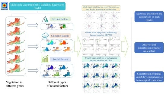
2.3.4. Multiscale Geographically Weighted Regression

GWR can effectively detect spatial non-stationarity by borrowing data from nearby sample points for parameter estimation. However, the bandwidth in the GWR model is the average of the different bandwidths of all independent variables, which leads to estimation bias [24,34]. As the latest improved version of the GWR model, the MGWR model simultaneously considers multiple bandwidths to address this shortcoming, thereby identifying the scale effects of different variables [24,35]. Therefore, this study intends to use the MGWR model to study the spatial non-stationarity and scale effects between the spatial distribution of vegetation in the YRB and other factors. The formula is as follows:
y i = j = 1 k β b w j ( u i , v i ) x i j + ε i  
In the formula: b w j   represents the bandwidth used by the jth variable regression coefficient. Each regression coefficient β b w j of MGWR is obtained based on local regression, and the bandwidth is specific, which is also the biggest difference from the classical GWR. In classical GWR, all variables of β b w j have the same bandwidth. The kernel function and bandwidth selection criteria of MGWR continue to use several classical kernel functions and bandwidth selection criteria of classic GWR. This paper used the most commonly used quadratic kernel function and AICc criterion.
MGWR can be equivalent to a generalized additive model (GAM) [25]. The formula is as follows:
y = j = 1 k f j + ε  
In the formula: f j represents the smoothing function of the jth independent variable. The smoothing function here used the Bi-square Kernel Function to calculate the optimal bandwidth [25,34,36]. The bandwidth can vary with the jth independent variable.
In this paper, the change ratio of the classical residual sum of squares (RSS) was used as the convergence criterion, and the formula was as follows:
S O C r s s = | R S S n e w + R S S o l d R S S n e w |  
In the formula: R S S o l d represented the residual sum of squares of the previous step; R S S n e w represented the residual sum of squares of this step.

3. Results

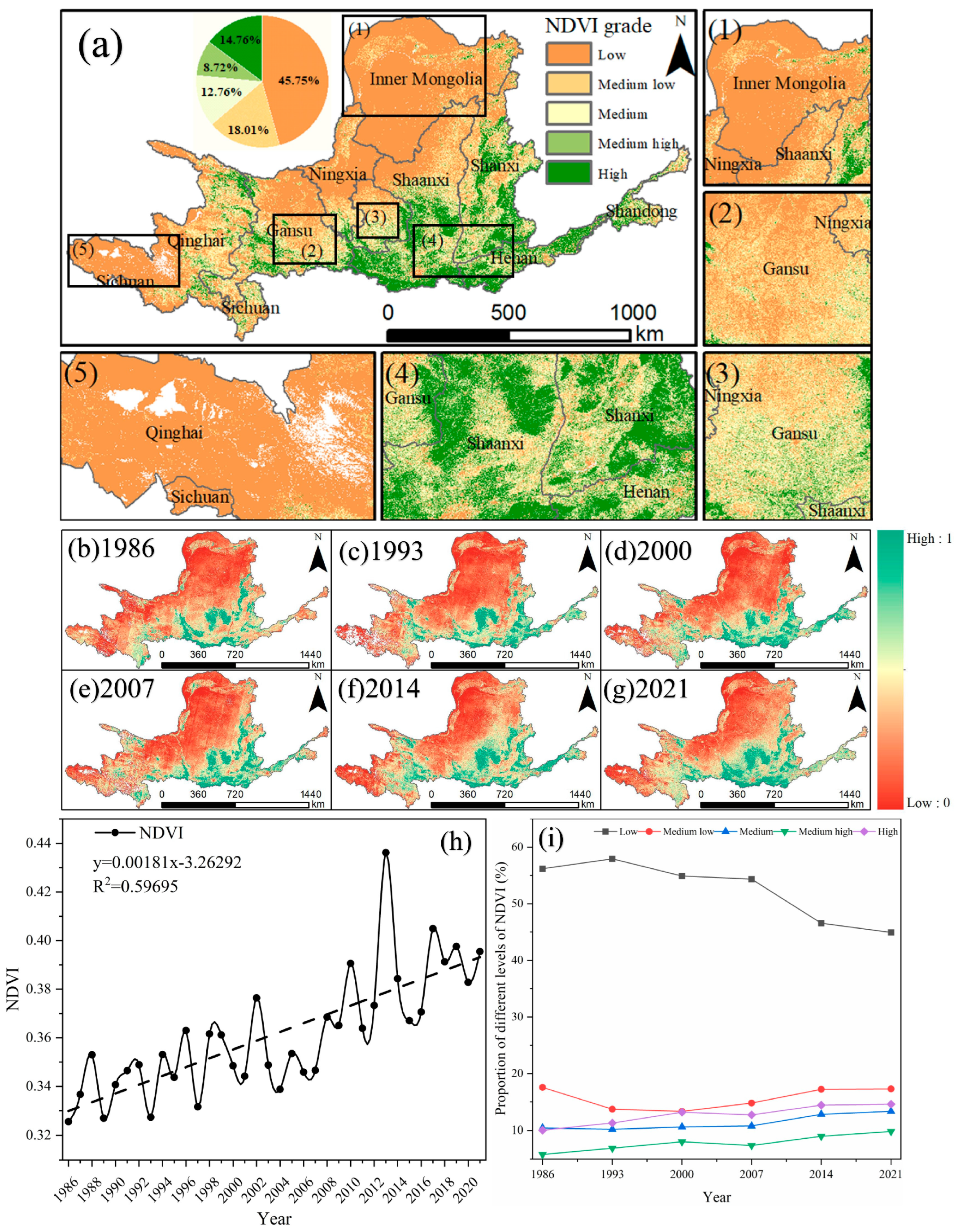
3.1. Spatial Distribution and Temporal Variation of Vegetation

(1) In general, vegetation in the YRB presented obvious spatial differentiation (Figure 2a). The proportion of low-grade NDVI was 45.75%, mainly located in the northwest of the YRB, such as Inner Mongolia, Ningxia, Gansu, Qinghai provinces. The high grades only accounted for 14.76%, distributed in the southeastern of YRB, such as Henan, Shaanxi, and Shanxi provinces;
(2) The vegetation of the YRB displayed an increased trend of fluctuation from 1986 to 2021 (Figure 2h), with a growth speed of 0.0018/year. The NDVI values in the past 36 years ranged from 0.3255 to 0.4049, indicating that the overall vegetation coverage was low. The NDVI in the southeastern part of the YRB gradually increased in six periods from the perspective of spatial distribution (Figure 2b–g), while the NDVI in the western part has been degrading. Vegetation in the middle of the basin showed a trend of degradation from 1986 to 2000, but improved from 2000 to 2007. These findings confirmed the vegetation existed large spatiotemporal heterogeneity in the YRB;
(3) As shown in Figure 2i, from 1986 to 2021, the area proportion of low-grade NDVI gradually decreased, from 56.18% to 44.93%. The area proportion of high-grade NDVI gradually increased from 10.03% to 14.60%. The area proportion of medium low NDVI showed a trend of decreasing first and then increasing, with the lowest proportion in 2000, only 13.32%.

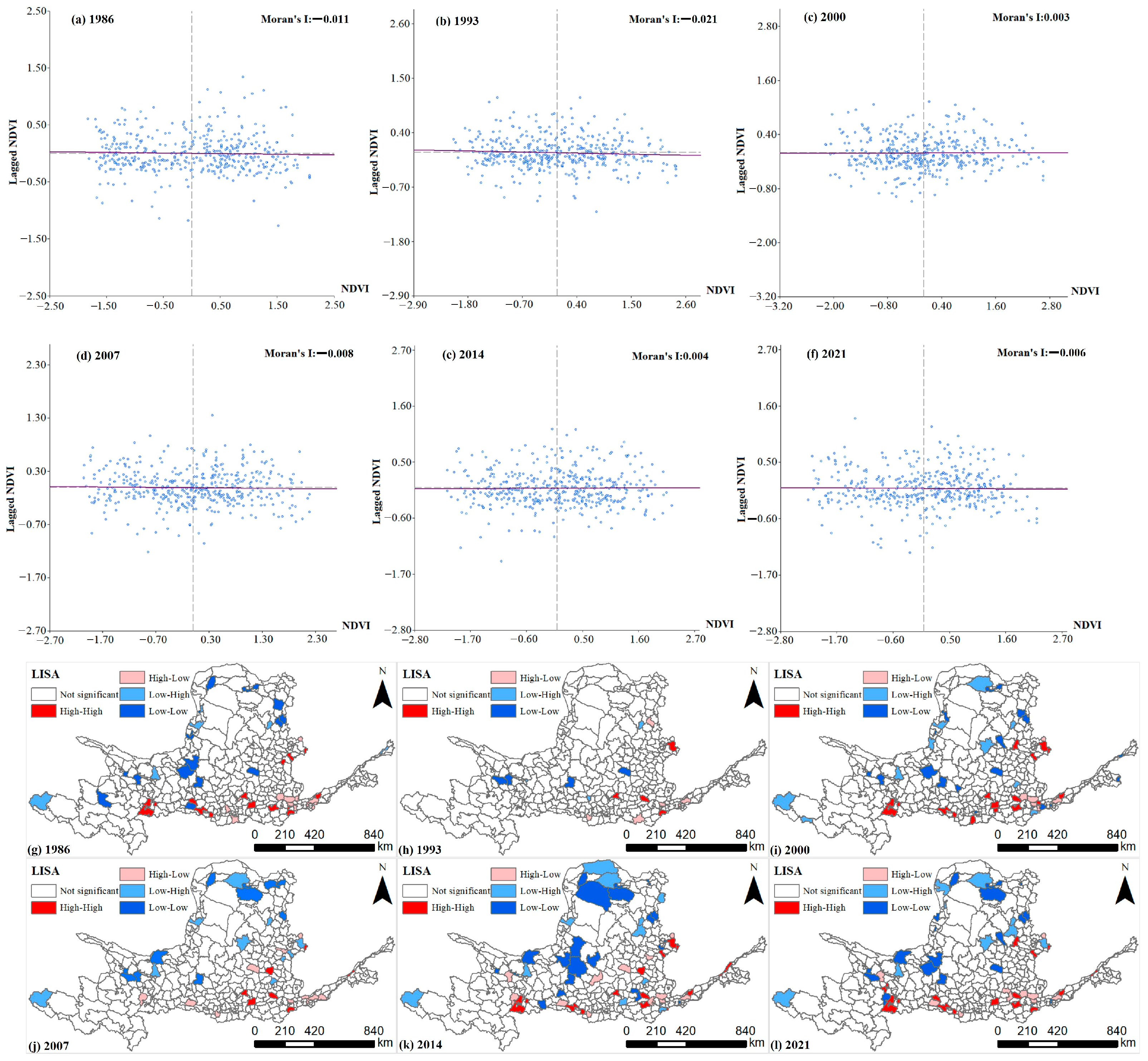
3.2. Spatial Autocorrelation of Vegetation

(1)
Global spatial autocorrelation of NDVI
The underlying idea behind the application of geographically weighted regression is that there is a spatial difference between the independent variable and the dependent variable connected to the geographic space, and as a result, the regression coefficient varies with the spatial location of the independent variable. Spatial autocorrelation analysis was done on NDVI in several years to see if the link between it and the outside environment was spatially stable. The findings demonstrated that the autocorrelation index of NDVI of YRB was not 0 (Figure 3a–f). NDVI in 1986, 1993, 2007, and 2021 exhibited negative spatial autocorrelation, as can be shown in Figure 3a–f. The geographical autocorrelation of the NDVI was positive between 2000 and 2014. The outcome demonstrated that the chosen parameters exhibited both positive and negative spatial autocorrelation, indicating that they were not stable in space. The quantitative effects of various environmental factors on NDVI in diverse geographic regions may thus be fully reflected by the geographical weighted regression technique;
(2)
Local spatial autocorrelation of NDVI
Utilizing regional Moran’ s I (LISA), the local spatial aggregation of NDVI in the YRB was further investigated (Figure 3g–l). The geographical clustering features of the NDVI from 1986 to 2021 indicated a considerable high-value spatial autocorrelation, which was high vegetation agglomeration, as can be observed from the LISA map of NDVI. Overall, each year’s vegetation aggregation is distributed spatially in a consistent manner. The northwest of the basin is where the “Low-Low” (LL) and “Low-High” (LH) cluster types are primarily found. The southwestern region of the basin is where the “High-High” (HH) and “High-Low” (HL) cluster types are found.

3.3. Model Comparison and Evaluation

Figure 4 compared the parameters of the MGWR and GWR. From the perspective of spatial distribution, the Local R2 value of MGWR (Figure 4b) was observably higher than the Local R2 value of GWR, while the Standard residual value of MGWR (Figure 4e) was comparable to that of GWR (Figure 4d). From a statistical point of view, there were significantly more cells with a Local R2 of 0.85–1.00 in MGWR than in GWR (Figure 4c), and the area of each interval value of the Standard residual of MGWR and GWR was equivalent (Figure 4f). In summary, although the Standard residual of GWR was comparable to that of MGWR, the Local R2 of MGWR was significantly better than that of GWR. This result indicated that MGWR had a stronger explanatory power for the spatial non-stationarity of vegetation and related factors. The MGWR model performed better data fitting than the GWR model because it took into consideration the varying effect scales of several influences on vegetation NDVI, which was supported by other research [24,37]. The scale disparities in each factor’s driving influence on vegetation must thus be taken into account in the future investigation.
Referring to previous studies [38], this paper selected R2, Adjusted R2, AIC, AICc, and RSS to compare the accuracy of OLS, GWR, MGWR models (Table 2). Comparative analysis revealed that the R2 (0.936) and Adjusted R2 (0.917) of the MGWR were significantly higher than the OLS’s (0.641, 0.631) and higher than those of the GWR (0.924, 0.895). The AICc (310.913) and RSS (28.389) of MGWR were much lower than the OLS model (838.250, 160.286) and lower than the GWR (483.333, 33.707). Therefore, it could be judged that the MGWR fared greater in terms of spatial elements’ goodness of fit. The result was also demonstrated by Sisman and Aydinoglu [26], Chang Chien et al. [39], Yang et al. [40] comparing the model superiority of OLS, GWR, and MGWR. Therefore, we chose to use the spatial regression results of MGWR to discuss the impact of various related factors on vegetation in the YRB and its spatial differences. Comparing the OLS, the results showed that the MGWR and GWR performed better than the OLS, considering the spatial scale and spatial non-stationarity, and possibly locate regional specifics that influence NDVI’s spatial variance. The use of variable bandwidth, which could reflect the varying degrees of effect of various factors on NDVI, gave the MGWR additional benefits [40].

3.4. The Global Scale of the Influencing Factors

The regression coefficients of each factor obtained by the MGWR were expressed in Figure 5. The positive and negative values indicated the direction of the effect, while the magnitude of the coefficient indicated the strength of the influence. Figure 5 not only showed the degree of effect of each factor on the vegetation in the Yellow River Basin, but also indicated the direction of the effect. In terms of influence degree, the overall influence degree of each factor on the YRB changed with time. For example, in 1986, SH had the greatest influence on vegetation, while in 1993, DEM was the strongest influence factor on vegetation. However, social factors had a very limited impact on vegetation at any time. In terms of impact direction, in general, the impact of PET on vegetation in the YRB was a single negative impact (except in 1986). The relationship between other factors and vegetation varied significantly over time. For example, NL had a single negative impact in 1986 and a single positive impact in 1993. GDP had a single negative effect in 1993 and 2007, and a single positive effect in 2014 and 2021.
It can be seen from the Table 3 that the p-values of each factor selected in this paper are close to 0.000. Only GDP and POP have relatively high p-values and relatively low significance.

3.5. Spatial Pattern of Regression Coefficients

The geographical variability of the interaction between variables and NDVI at various spatial locations was recognized by the MGWR model. The model’s output showed the geographical distribution of the regression coefficients for each component (Figure 6). The regression coefficient’s absolute value showed the factor’s level of effect over vegetation, and its positive and negative values indicated the direction of that influence. The geographical differentiation impact of vegetation and related elements in the counties of the YRB was explained in this section using the output coefficient of the MGWR model in 2021 as an example.
In terms of topography, the Slope had a little detrimental effect on the vegetation in the allied counties of Lanzhou, Xi’an, Zhengzhou, and Jinan. The vegetation of subordinate counties of Xining, Hohhot, and Taiyuan was positively affected by Slope (Figure 6a). DEM had a strong negative effect on vegetation in the YRB (except for four counties near Xining City). The maximum degree of influence of DEM could reach −2.301 (Figure 6b), and it was mainly distributed in thirteen counties near Ordos City.
In terms of meteorology, the spatial relationship between NDVI and PRE was mainly positive, and only the 30 counties in the lower reaches of the basin were negative (Figure 6c). Unlike PRE, TEM had a larger and single positive impact on NDVI (Figure 6d), and the high-altitude areas in the upstream of the basin were most affected by TEM. The impact of PET on vegetation in the YRB gradually decreased from west to east (Figure 6e), and the impact degree was below −1.600. RH only had a small positive influence on vegetation in 8 counties of Linfen City (Figure 6f), but had a negative effect on other counties in the YRB. The central zone of the YRB was negatively impacted by SH, and the districts and counties in the Guanzhong urban agglomeration and Hu-Bao and E-Yu urban agglomeration were most affected by SH, ranging from −1.077 to −0.691.
In terms of social impact, the effect of GDP on vegetation in the YRB decreased from west to east (Figure 6h), and the degree of impact was relatively small (≤0.026). Different from GDP, the impact of POP performed a declining tendency from north to south (Figure 6i), and the impact was relatively small. The effect of D-river on the counties of Shaanxi and Gansu in the central part of the basin and the counties of Xining and Yushu in Qinghai was a negative effect to a low degree (−0.137~0.000) (Figure 6j). Vegetation in the YRB was mainly negatively affected by D-residence (Figure 6k), and the effect intensity was low. Only the districts and counties under the Jinzhong urban agglomeration were positively affected. NL and the vegetation of the YRB showed a gradually decreasing spatial correlation from north to south (Figure 6l). Only the urban agglomeration of Hu-Bao and E-Yu was positively affected by NL.

4. Discussion

4.1. Contribution of Spatial Variability of Different Factors to Ecological Restoration of Vegetation

Global scale analysis found that the key variables influencing NDVI in the YRB were temperature and elevation (Figure 5), and previous studies also found the same conclusion [19,41]. This study also discovered that societal influences had a minimal overall impact on the vegetation in the YRB. This result may be due to the fact that the YRB was located in an underdeveloped area in central and western China, and the level and rate of socioeconomic development were relatively low. Different from the OLS global regression model, the MGWR model could intuitively reflect the regression coefficients of various factors and vegetation in space [38]. From the analysis of the MGWR output results, it was known that the vegetation in various areas of the YRB (county-level unit scale) varied spatially in the strength of the effects of various causes (Figure 6). The factor with the largest absolute value of the regression coefficient was considered as the decisive factor for the location. Figure 7 showed the spatiotemporal heterogeneity of the determinants of vegetation in the YRB, with different colors representing different factors. This study also provided different vegetation ecological restoration policy support for different regions (districts and counties) in the YRB at different time periods. Therefore, the ecological engineering measures must be adjusted taking into account the geographical variations in the key elements of plant restoration. The ecological engineering measures must be adjusted taking into account the geographical variations in the key elements of plant restoration.
(1)
The influence of terrain factors on vegetation
The study discovered that topography had a major effect on the vegetation of the YRB. (Figure 6a,b). The degree of effect increases with the regression coefficient’s absolute magnitude. DEM had a substantially bigger impact on NDVI than slope [42]. As a critical condition factor of vegetation change, altitude indirectly affected the growth and change of vegetation by regulating the hydrothermal conditions and nutrient organic matter required by plants [4,43,44]. In addition, altitude also indirectly affects vegetation changes by affecting human activities. Figure 6b showed that vegetation in low-altitude areas such as the Hetao Plain, the Guanzhong Plain, and the North China Plain was strongly affected. This result was mainly due to the low altitude, which was suitable for human social development [45] and agricultural reclamation [46], resulting in relatively low vegetation cover.
Therefore, in the formulation of vegetation ecological restoration policies in the future, we should focus on the lower-elevation plain areas of which the Hetao Plain was the most critical (Figure 7). The north bank of the Yellow River in this plain had flat terrain and fertile soil and was an important grain-producing area [47]. However, the south bank of the Yellow River had a greater elevation than the north bank, had major soil erosion, had virtually little plant cover, and was mostly used for desert (Figure 1c). Therefore, for the south bank, afforestation should be the main focus, and grazing and agricultural reclamation should be reduced [48]. Although the north bank was a food-producing area, the vegetation cover was also relatively low and at risk of further degradation;
(2)
The influence of climate factors on vegetation
In terms of the degree of influence, PET had the largest impact on NDVI, the absolute values of the regression coefficients clustered in the range of 1.588–1.724 in the YRB (Figure 6e and Figure 5f). The finding was in line with the research done by Yang et al. [1]. In arid and semi-arid regions, Evapotranspiration was the main route of water consumption in the water cycle [49]. The increase in evaporation caused a significant loss of soil moisture, which exacerbated the drought and gradually reduced the amount of water available for plant development [50]. In addition, with the increase of PET, the surface dryness increased, and strong wind, precipitation, and high sun radiation all damaged the exposed soil. The root grip of vegetation decreased, which further led to the increase of PET in the deep soil layer [51]. Therefore, vegetation in the YRB, which was mainly arid and semi-arid, gradually degenerated with the increase of evapotranspiration.
Unlike PET, TEM showed a strong one-way positive effect on vegetation in the YRB, that was, NDVI increased with temperature (Figure 6d), which was also supported by previous studies [19,48]. The effect of TEM on vegetation was seen as a regional distinction that gradually dwindled from west to east from the standpoint of spatial dispersion. The study results showed that the Qinghai-Tibet Plateau regions in the west were most affected by temperature, which may be due to the increased photosynthesis of forest vegetation in high-altitude areas [1,52]. On the other hand, the permafrost in this region was deteriorated, the freezing and thawing times were decreased, and the soil moisture was replenished by the temperature increase. The vegetation’s germination period was brought forward and the deciduous period was delayed, which increased the vegetation’s growth period and promoted the prosperity of the vegetation [53,54].
As another necessary condition for the photosynthesis of plants (SH) [48], its impact on vegetation in the YRB was second only to PET and TEM. The study found that the areas, where the vegetation was positively affected by SH were mainly high-altitude areas, such as the southern foot of the Qilian Mountains and the eastern Qinghai-Tibet Plateau (Figure 6g). This outcome was mostly caused by the fact that plant absorbs more solar energy in colder climates, particularly in the Qilian Mountains region, where the yearly average temperature was below 7 °C. Reduced surface albedo had a favorable impact on the NDVI greening [1,55].
Previous studies mostly believed that precipitation was largely considered to be a major component influencing plant development [47]. However, we found that the influence of precipitation relative to other climatic factors was lower, which may be related to the YRB’s predominant grassland vegetation type. Therefore, the sensitivity to precipitation was not as strong as other vegetation types [43]. In terms of the direction of influence, the vegetation in the lower reaches of the basin was negatively affected by precipitation (Figure 6c), which may be due to the fact that the region was in a humid or semi-humid area, and excessive precipitation inhibited the growth of vegetation [48]. Different from precipitation, the study found that the impact of RH on vegetation was mainly negative (Figure 5f and Figure 6f), and previous studies also found similar conclusions [56].
Low tree survival rates are the outcome of the predilection for exotic species throughout the afforestation process, which frequently overlooked the real local natural circumstances [11]. Given the variations in how various climate elements affect the vegetation in the YRB, vegetation ecological restoration policies should be formulated to deal with different climate changes. Figure 7 demonstrated that at the middle and lower portions of the YRB, PET had the greatest influence on the vegetation. Different plant varieties were shown to have varying levels of resistance to evapotranspiration in earlier research [1]. Therefore, the selection of plants adapted to high evapotranspiration was crucial for the ecological restoration of the YRB. For example, shrubs with lower plants may be able to withstand the impacts of increased evapotranspiration by thinning stems and petioles, dwarfing the structure, and rolling up leaves to minimize leaf area. TEM was a key influencing factor of NDVI on the QTP, the relationship between TEM and vegetation in this area was positively correlated (Figure 6d). Therefore, in the face of the global warming environment, the vegetation in this area will gradually develop for the better [6]. Reducing excessive external intervention, allowing it to develop freely or establishing a natural ecological reserve may be the best solution for the continuous increase of vegetation coverage;
(3)
The influence of social factors on vegetation
This study found significant differences in the ways in which social and natural factors affected NDVI (Figure 6). Previous studies generally believed that vegetation was impacted more by social than by natural reasons. However, this paper found that human socioeconomic variables had a substantially less influence on vegetation than did natural causes, which was also consistent with the global impact analysis results derived from OLS (Figure 5). In terms of the influence direction, social and economic factors had positive and negative spatial non-stationarity on the vegetation in the YRB. For example, NL had an advantageous effect on the NDVI of the Ordos-Hohhot urban agglomeration in the northwest of the YRB (Figure 6l), while it had a detrimental effect on the plants in other areas. This result may be due to the YRB’s uneven degree of regional economic development. The higher the Northwest NL in the less developed regions, the more adequate the funds available for revegetation policies. However, the Guanzhong Plain urban agglomeration, which was relatively developed, has a detrimental impact on vegetation because of the continuous development of cities [56].
The regression coefficients of NL and POP had the similar geographic distribution pattern (Figure 6i,l), which may be due to the fact that the spatial trends of POP and NL were related to the spatial pattern of urbanization development. Previous studies suggested that GDP and NL also had comparable spatial distribution patterns [38]. However, this paper obtained different results (Figure 6h), that was, the vegetation in the YRB was affected by a single positive effect of GDP. This result may be due to the fact that the economic development level of most areas in the YRB was not as good as that of coastal cities. The investment funds available for ecological restoration of vegetation were relatively limited. With the growth of GDP, the funds for vegetation restoration projects had increased relatively, which in turn led to the improvement of vegetation. Therefore, the regression coefficient between vegetation and GDP presented a single positive.
The findings indicated that D-residence had a largely negative effect on vegetation, that was, with the increase of distance from residential areas, NDVI gradually decreased. This conclusion may be due to the reduction of human accessibility and the reduction of policy implementation for vegetation restoration. Therefore, the vegetation cover gradually decreased with D-residence. Previous studies generally believed that proximity to water sources could promote vegetation growth [45]. However, this study found the opposite conclusion, that was, the NDVI was lower for vegetation close to the water source. This result might be attributed to the YRB’s distribution of human activity regions around water supplies, including metropolitan centers, cities, villages, and industry. The closer humans were to water sources, the greater the impact on vegetation. Therefore, D-river and NDVI had a positive correlation.
Although vegetation was less affected by social factors than natural factors in the YRB, economic and social development provided financial support for the implementation of vegetation ecological restoration policies. Therefore, when carrying out ecological restoration, it was vital to fully consider the geographical variances in the influence of factors such as the socio-economic development of the YRB on vegetation growth. For example, the northwest of the basin with low economic development level was also the area with the lowest vegetation coverage in the YRB (Figure 2b–g), and ecological restoration was imminent. Although the northwest has been returning farmland to forest and grassland for many years, the vegetation improvement here was not significant (Figure 2b–g). This finding may be due to the remote geographical location of the northwestern part of the YRB (Figure 1b) and inconvenient transportation, it was difficult to effectually monitor the implementation effect of ecological projects [57]. Although returning farmland to forests had established economic benchmarks for farmer subsidies, due to the northwest’s relatively low degree of economic growth, the number of subsidies was limited, and reclamation was likely to occur after expiration [11]. In addition, ecological engineering was inefficient due to excessive administrative intervention in the afforestation model, planting just one type of tree or introducing plants that did not conform to local natural conditions [11,58]. These factors caused the unsustainable development of vegetation cover, all of which deserved great attention from policymakers. As previous studies suggested, enough attractive subsidies should be provided to farmers, and incentive policies should be used to promote farmers’ active participation in ecological construction [59].

4.2. Scale Effect Analysis of Vegetation and Other Factors

The variance in the bandwidth of all variables between the GWR and MGWR in various years was presented in Figure 8. The bandwidth used in the models can be seen as a scale of influence of different variables. While GWR can only represent the average value of each variable’s effect scale, MGWR may directly reflect the differential action scale of many variables (Figure 8). Through MGWR data, it was discovered that the degree of action of several factors differed considerably. For example, the impact scale of each variable on vegetation was local scale in 1986, among which the response scale of DEM, PRE, RH, SH, and GDP was 43, the scale of Slope and D-river was 44, and the scale of PET and POP was 87. TEM, D-residence, and NL had scales of 75, 129, and 141, respectively. With the change of time, the effect scales of different influencing factors have changed to different degrees. For example, the spatial correlation scale of Slope and vegetation fluctuates only slightly, between 43–45. The action scale of PRE changed from a local scale (43) to a global scale (445) from 1986 to 1993.
(1)
Scale variability was analyzed from different factor perspectives
The scale coefficients derived from the MGWR model can be used to identify different areas of effect of different factors on vegetation. The global robustness of some variables is ignored when using the GWR model [23], and the scale of the action of all factors on vegetation was only a single optimal mean scale (Figure 8). The difference in the scale of action of different factors was often ignored, which led to the misleading conclusion that the spatial non-stationarity was not significant [34]. Different from GWR, the study results of MGWR showed that the effect scale of different environmental factors on vegetation in the YRB was significantly different. The scale of vegetation affected by the terrain factor (slope elevation) was relatively low, such as the scale of Slope, which was 43. However, the scale of meteorological data on vegetation was relatively large, for example, the scale of precipitation was 445. The findings demonstrated that the effect of terrain factors on vegetation was very local (smaller bandwidth) compared to meteorological factors. Cost-effective land cover planning was aided by this accurate identification of spatial-scale relationships [60]. Developing vegetation restoration policies from this perspective should focus on inter-regional characteristics.
The policy of vegetation ecological restoration can be made according to the scale difference of different factors. Accordingly, the benefits of layer-by-layer division in the joint governance approach may be compared to the advantages of MGWR’s spatial action scale division in this study. Another benefit is that regional joint governance, as opposed to global single governance, allows for more precise management decisions [38]. For example, vegetation was affected by 43 nearby terrain units, so 43 terrain units could be combined as the minimum area for the implementation of the corresponding vegetation policy. This method avoided the global implementation of the same policy and reduced the waste of resources due to policy implementation overflow. Vegetation was affected by 129 nearby D-residence units. Therefore, when formulating vegetation restoration policies, the effect of residential areas in 129 nearby districts and counties on vegetation should be considered;
(2)
The spatial scale dependence of vegetation and other factors varied with the interannual variation
Most previous studies believed that the scale of the spatial relationship between vegetation and related factors remained unchanged [45,61]. However, the results in Figure 8 indicate that the spatial scale of vegetation and other factors varied over time. Yang et al. [1] also found that temporal and spatial changes could change the response mechanism of vegetation to driving factors. This study found that the scale of action between vegetation and social factors in the YRB fluctuated greatly over time. For example, the effective scale of GDP on NDVI increased from 43 in 1986 to 445 in 2000, dropped to 295 in 2007, and rose to 445 in 2014 and 2021. Fluctuations in this scale relationship also force relevant departments to continuously update vegetation restoration policies over time.

5. Conclusions

This study analyzed the spatial and temporal distribution characteristics of NDVI in the YRB during 1986–2021. The spatial non-stationarity of NDVI and different types of factors (terrain, climatic and social) were discussed by MGWR. The results of MGWR were compared with those of the GWR and OLS models. This study found:
  • In the YRB, the northwest had a low NDVI, while the southeast had a high NDVI. In the past 36 years, the vegetation had a 0.0018-per-year fluctuating increasing trend. The results of the NDVI agglomeration model showed that the H-H and H-L agglomeration model units were primarily positioned in the southeast, and the L-L and L-H agglomeration units were located in the northwest region;
  • Compared with the global linear model OLS and classical GWR, the results of MGWR were more reliable. The result was mainly due to the fact that MGWR can capture different influence scales of different variables, thus avoiding capturing too much noise and bias, and having better robustness. Therefore, whether the spatial scale of the affecting variables was considered would have a significant influence on the results of the model;
  • The scale of the effect of each factor on vegetation was obviously different. Vegetation was very sensitive to terrain factors and had strong spatial non-stationarity. The scale of the effect of DEM was the smallest of all variables at 43. Other factors were Slope, SH, RH, GDP, D-river, TEM, PET, POP, D-residence, and NL according to their spatial scales from small to large. This scaling relationship also fluctuated over time;
  • The response process between vegetation and various driving factors exhibited significant spatial non-stationarity. It is worth noting that in addition to the impact of climate variables, such as PET, TEM, SH and RH, the influence of DEM on the vegetation in the YRB should not be underestimated. However, social factors, such as GDP, POP, and NL, had a negligible effect on the vegetation. These results further confirmed that the MGWR model could be applied to similar studies dealing with non-stationary features, such as human activities and environmental changes, in order to capture both time and space non-stationarity.
This study evaluated the magnitude of each factor’s impact on vegetation in order to identify the key influences on vegetation from both a quantitative and intuitive standpoint. This paper offered fresh information that may be used in the future to make informed decisions in the YRB and to solve the vegetation ecological restoration problem scientifically. Therefore, this study promoted the high-quality development of the ecological environment quality of the YRB. In the future, we will consider more different types of factors (such as snow cover, the number of days with precipitation and abnormal temperature) to study the impact of vegetation.

Author Contributions

Conceptualization, X.W.; methodology, X.W. and S.S.; software, S.S. and M.H.; validation, S.S. and X.Z.; formal analysis, S.S.; data curation, Z.H.; writing—original draft preparation, S.S.; writing—review and editing, S.S. and X.W.; project administration, X.W. and L.X. All authors have read and agreed to the published version of the manuscript.

Funding

This research was funded by the key scientific and technological project of Henan Province, grant number 212102210137; the Natural Science Foundation of Henan, grant number 212300410292; the key research project of higher Education of Henan Province, China, grant number 21A420006; and the Open Fund of National Engineering Research Center for Geographic Information System, China University of Geosciences, Wuhan 430074, China, grant number 2021KFJJ04.

Institutional Review Board Statement

Not applicable.

Informed Consent Statement

Not applicable.

Data Availability Statement

Not applicable.

Conflicts of Interest

The authors declare no conflict of interest.

References

  1. Yang, L.; Guan, Q.; Lin, J.; Tian, J.; Tan, Z.; Li, H. Evolution of NDVI secular trends and responses to climate change: A perspective from nonlinearity and nonstationarity characteristics. Remote Sens. Environ. 2021, 254, 112247. [Google Scholar] [CrossRef]
  2. Gampe, D.; Zscheischler, J.; Reichstein, M.; O’Sullivan, M.; Smith, W.K.; Sitch, S.; Buermann, W. Increasing impact of warm droughts on northern ecosystem productivity over recent decades. Nat. Clim. Chang. 2021, 11, 772–779. [Google Scholar] [CrossRef]
  3. Zhong, Q.; Ma, J.; Zhao, B.; Wang, X.; Zong, J.; Xiao, X. Assessing spatial-temporal dynamics of urban expansion, vegetation greenness and photosynthesis in megacity Shanghai, China during 2000–2016. Remote Sens. Environ. 2019, 233, 111374. [Google Scholar] [CrossRef]
  4. Gao, M.; Piao, S.; Chen, A.; Yang, H.; Liu, Q.; Fu, Y.H.; Janssens, I.A. Divergent changes in the elevational gradient of vegetation activities over the last 30 years. Nat. Commun. 2019, 10, 2970. [Google Scholar] [CrossRef] [PubMed] [Green Version]
  5. Mayor, J.R.; Sanders, N.J.; Classen, A.T.; Bardgett, R.D.; Clement, J.C.; Fajardo, A.; Lavorel, S.; Sundqvist, M.K.; Bahn, M.; Chisholm, C.; et al. Elevation alters ecosystem properties across temperate treelines globally. Nature 2017, 542, 91–95. [Google Scholar] [CrossRef] [Green Version]
  6. Huang, M.; Piao, S.; Janssens, I.A.; Zhu, Z.; Wang, T.; Wu, D.; Ciais, P.; Myneni, R.B.; Peaucelle, M.; Peng, S.; et al. Velocity of change in vegetation productivity over northern high latitudes. Nat. Ecol. Evol. 2017, 1, 1649–1654. [Google Scholar] [CrossRef] [Green Version]
  7. Chen, C.; Park, T.; Wang, X.; Piao, S.; Xu, B.; Chaturvedi, R.K.; Fuchs, R.; Brovkin, V.; Ciais, P.; Fensholt, R.; et al. China and India lead in greening of the world through land-use management. Nat. Sustain. 2019, 2, 122–129. [Google Scholar] [CrossRef]
  8. Smith, T.; Traxl, D.; Boers, N. Empirical evidence for recent global shifts in vegetation resilience. Nat. Clim. Chang. 2022, 12, 477–484. [Google Scholar] [CrossRef]
  9. Zhang, D.; Geng, X.; Chen, W.; Fang, L.; Yao, R.; Wang, X.; Zhou, X. Inconsistency of Global Vegetation Dynamics Driven by Climate Change: Evidences from Spatial Regression. Remote Sens. 2021, 13, 3442. [Google Scholar] [CrossRef]
  10. Zuo, D.; Han, Y.; Xu, Z.; Li, P.; Ban, C.; Sun, W.; Pang, B.; Peng, D.; Kan, G.; Zhang, R.; et al. Time-lag effects of climatic change and drought on vegetation dynamics in an alpine river basin of the Tibet Plateau, China. J. Hydrol. 2021, 600, 126532. [Google Scholar] [CrossRef]
  11. He, J.; Shi, X.; Fu, Y. Identifying vegetation restoration effectiveness and driving factors on different micro-topographic types of hilly Loess Plateau: From the perspective of ecological resilience. J. Environ. Manag. 2021, 289, 112562. [Google Scholar] [CrossRef] [PubMed]
  12. Feng, D.; Yang, C.; Fu, M.; Wang, J.; Zhang, M.; Sun, Y.; Bao, W. Do anthropogenic factors affect the improvement of vegetation cover in resource-based region? J. Clean. Prod. 2020, 271, 122705. [Google Scholar] [CrossRef]
  13. Yang, L.; Shen, F.; Zhang, L.; Cai, Y.; Yi, F.; Zhou, C. Quantifying influences of natural and anthropogenic factors on vegetation changes using structural equation modeling: A case study in Jiangsu Province, China. J. Clean. Prod. 2021, 280, 124330. [Google Scholar] [CrossRef]
  14. Zhang, W.; Randall, M.; Jensen, M.B.; Brandt, M.; Wang, Q.; Fensholt, R. Socio-economic and climatic changes lead to contrasting global urban vegetation trends. Glob. Environ. Chang. 2021, 71, 102385. [Google Scholar] [CrossRef]
  15. Zhang, L.; Sun, P.; Huettmann, F.; Liu, S. Where should China practice forestry in a warming world? Glob. Chang. Biol. 2021, 28, 2461–2475. [Google Scholar] [CrossRef]
  16. Piao, S.; Wang, X.; Park, T.; Chen, C.; Lian, X.; He, Y.; Bjerke, J.W.; Chen, A.; Ciais, P.; Tømmervik, H.; et al. Characteristics, drivers and feedbacks of global greening. Nat. Rev. Earth Environ. 2019, 1, 14–27. [Google Scholar] [CrossRef] [Green Version]
  17. Zhang, W.; Wang, L.; Xiang, F.; Qin, W.; Jiang, W. Vegetation dynamics and the relations with climate change at multiple time scales in the Yangtze River and Yellow River Basin, China. Ecol. Indic. 2020, 110, 105892. [Google Scholar] [CrossRef]
  18. Jiang, W.; Niu, Z.; Wang, L.; Yao, R.; Gui, X.; Xiang, F.; Ji, Y. Impacts of Drought and Climatic Factors on Vegetation Dynamics in the Yellow River Basin and Yangtze River Basin, China. Remote Sens. 2022, 14, 930. [Google Scholar] [CrossRef]
  19. Tian, F.; Liu, L.-Z.; Yang, J.-H.; Wu, J.-J. Vegetation greening in more than 94% of the Yellow River Basin (YRB) region in China during the 21st century caused jointly by warming and anthropogenic activities. Ecol. Indic. 2021, 125, 107479. [Google Scholar] [CrossRef]
  20. Brunsdon, C.; Fotheringham, A.; Charlton, M. Geographically Weighted Regression: A Method for Exploring Spatial Nonstationarity. Geogr. Anal. 1996, 28, 281–298. [Google Scholar] [CrossRef]
  21. Jiao, K.; Gao, J.; Liu, Z. Precipitation Drives the NDVI Distribution on the Tibetan Plateau While High Warming Rates May Intensify Its Ecological Droughts. Remote Sens. 2021, 13, 1305. [Google Scholar] [CrossRef]
  22. Birhanu, A.; Adgo, E.; Frankl, A.; Walraevens, K.; Nyssen, J. Modelling spatial relationships between land cover change and its drivers in the Afro-alpine belt of Mount Guna (Ethiopia). Land Degrad. Dev. 2021, 32, 3946–3961. [Google Scholar] [CrossRef]
  23. Niu, L.; Zhang, Z.; Peng, Z.; Liang, Y.; Liu, M.; Jiang, Y.; Wei, J.; Tang, R. Identifying Surface Urban Heat Island Drivers and Their Spatial Heterogeneity in China’s 281 Cities: An Empirical Study Based on Multiscale Geographically Weighted Regression. Remote Sens. 2021, 13, 4428. [Google Scholar] [CrossRef]
  24. Fotheringham, A.S.; Yu, H.; Wolf, L.J.; Oshan, T.M.; Li, Z. On the notion of ‘bandwidth’ in geographically weighted regression models of spatially varying processes. Int. J. Geogr. Inf. Sci. 2022, 36, 1485–1502. [Google Scholar] [CrossRef]
  25. Li, Z.; Fotheringham, A.S. Computational improvements to multi-scale geographically weighted regression. Int. J. Geogr. Inf. Sci. 2020, 34, 1378–1397. [Google Scholar] [CrossRef]
  26. Sisman, S.; Aydinoglu, A.C. A modelling approach with geographically weighted regression methods for determining geographic variation and influencing factors in housing price: A case in Istanbul. Land Use Policy 2022, 119, 106183. [Google Scholar] [CrossRef]
  27. Jia, J.; Zhang, X.; Huang, C.; Luan, H. Multiscale analysis of human social sensing of urban appearance and its effects on house price appreciation in Wuhan, China. Sustain. Cities Soc. 2022, 81, 103844. [Google Scholar] [CrossRef]
  28. Tran, D.X.; Pearson, D.; Palmer, A.; Lowry, J.; Gray, D.; Dominati, E.J. Quantifying spatial non-stationarity in the relationship between landscape structure and the provision of ecosystem services: An example in the New Zealand hill country. Sci. Total Environ. 2021, 808, 152126. [Google Scholar] [CrossRef]
  29. Li, W.; Dong, F.; Ji, Z. Research on coordination level and influencing factors spatial heterogeneity of China’s urban CO2 emissions. Sustain. Cities Soc. 2021, 75, 103323. [Google Scholar] [CrossRef]
  30. Ran, C.; Wang, S.; Bai, X.; Tan, Q.; Wu, L.; Luo, X.; Chen, H.; Xi, H.; Lu, Q. Evaluation of temporal and spatial changes of global ecosystem health. Land Degrad. Dev. 2020, 32, 1500–1512. [Google Scholar] [CrossRef]
  31. Lin, T.; Xu, J.; Shen, X.; Jiang, H.; Zhong, R.; Wu, S.; Du, Z.; Rodriguez, L.; Ting, K.C. A spatiotemporal assessment of field residues of rice, maize, and wheat at provincial and county levels in China. GCB Bioenergy 2019, 11, 1146–1158. [Google Scholar] [CrossRef]
  32. Koh, E.H.; Lee, E.; Lee, K.K. Application of geographically weighted regression models to predict spatial characteristics of nitrate contamination: Implications for an effective groundwater management strategy. J. Environ. Manag. 2020, 268, 110646. [Google Scholar] [CrossRef]
  33. Feng, L.; Wang, Y.; Zhang, Z.; Du, Q. Geographically and temporally weighted neural network for winter wheat yield prediction. Remote Sens. Environ. 2021, 262, 111374. [Google Scholar] [CrossRef]
  34. Fotheringham, A.S.; Yang, W.; Kang, W. Multiscale Geographically Weighted Regression (MGWR). Ann. Am. Assoc. Geogr. 2017, 107, 1247–1265. [Google Scholar] [CrossRef]
  35. Wu, C.; Ren, F.; Hu, W.; Du, Q. Multiscale geographically and temporally weighted regression: Exploring the spatiotemporal determinants of housing prices. Int. J. Geogr. Inf. Sci. 2018, 33, 489–511. [Google Scholar] [CrossRef]
  36. Li, Z.; Fotheringham, A.S.; Li, W.; Oshan, T. Fast Geographically Weighted Regression (FastGWR): A scalable algorithm to investigate spatial process heterogeneity in millions of observations. Int. J. Geogr. Inf. Sci. 2019, 33, 155–175. [Google Scholar] [CrossRef]
  37. Lin, J.; Wang, Q.; Li, X. Socioeconomic and spatial inequalities of street tree abundance, species diversity, and size structure in New York City. Landsc. Urban Plan. 2021, 206, 103992. [Google Scholar] [CrossRef]
  38. Wu, T.; Zhou, L.; Jiang, G.; Meadows, M.E.; Zhang, J.; Pu, L.; Wu, C.; Xie, X. Modelling Spatial Heterogeneity in the Effects of Natural and Socioeconomic Factors, and Their Interactions, on Atmospheric PM2.5 Concentrations in China from 2000–2015. Remote Sens. 2021, 13, 2152. [Google Scholar] [CrossRef]
  39. Chang Chien, Y.-M.; Carver, S.; Comber, A. Using geographically weighted models to explore how crowdsourced landscape perceptions relate to landscape physical characteristics. Landsc. Urban Plan. 2020, 203, 103992. [Google Scholar] [CrossRef]
  40. Yang, L.; Yu, K.; Ai, J.; Liu, Y.; Yang, W.; Liu, J. Dominant Factors and Spatial Heterogeneity of Land Surface Temperatures in Urban Areas: A Case Study in Fuzhou, China. Remote Sens. 2022, 14, 1266. [Google Scholar] [CrossRef]
  41. Cui, J.; Zhu, M.; Liang, Y.; Qin, G.; Li, J.; Liu, Y. Land Use/Land Cover Change and Their Driving Factors in the Yellow River Basin of Shandong Province Based on Google Earth Engine from 2000 to 2020. ISPRS Int. J. Geo-Inf. 2022, 11, 163. [Google Scholar] [CrossRef]
  42. Wang, B.; Xu, G.; Li, P.; Li, Z.; Zhang, Y.; Cheng, Y.; Jia, L.; Zhang, J. Vegetation dynamics and their relationships with climatic factors in the Qinling Mountains of China. Ecol. Indic. 2020, 108, 105719. [Google Scholar] [CrossRef]
  43. Liu, C.; Li, W.; Wang, W.; Zhou, H.; Liang, T.; Hou, F.; Xu, J.; Xue, P. Quantitative spatial analysis of vegetation dynamics and potential driving factors in a typical alpine region on the northeastern Tibetan Plateau using the Google Earth Engine. Catena 2021, 206, 105500. [Google Scholar] [CrossRef]
  44. Li, S.F.; Valdes, P.J.; Farnsworth, A.; Davies-Barnard, T.; Su, T.; Lunt, D.J.; Spicer, R.A.; Liu, J.; Deng, W.Y.; Huang, J.; et al. Orographic evolution of northern Tibet shaped vegetation and plant diversity in eastern Asia. Sci. Adv. 2021, 7, eabc7741. [Google Scholar] [CrossRef] [PubMed]
  45. Chen, L.; Zhang, H.; Zhang, X.; Liu, P.; Zhang, W.; Ma, X. Vegetation changes in coal mining areas: Naturally or anthropogenically Driven? Catena 2022, 208, 105712. [Google Scholar] [CrossRef]
  46. Xiong, Y.; Li, Y.; Xiong, S.; Wu, G.; Deng, O. Multi-scale spatial correlation between vegetation index and terrain attributes in a small watershed of the upper Minjiang River. Ecol. Indic. 2021, 126, 107610. [Google Scholar] [CrossRef]
  47. Deng, X.; Hu, S.; Zhan, C. Attribution of vegetation coverage change to climate change and human activities based on the geographic detectors in the Yellow River Basin, China. Environ. Sci. Pollut. Res. 2022, 29, 44693–44708. [Google Scholar] [CrossRef]
  48. Ge, W.; Deng, L.; Wang, F.; Han, J. Quantifying the contributions of human activities and climate change to vegetation net primary productivity dynamics in China from 2001 to 2016. Sci. Total Environ. 2021, 773, 145648. [Google Scholar] [CrossRef]
  49. Zhao, F.; Ma, S.; Wu, Y.; Qiu, L.; Wang, W.; Lian, Y.; Chen, J.; Sivakumar, B. The role of climate change and vegetation greening on evapotranspiration variation in the Yellow River Basin, China. Agric. For. Meteorol. 2022, 316, 108842. [Google Scholar] [CrossRef]
  50. Li, Y.; Piao, S.; Li, L.Z.X.; Chen, A.; Wang, X.; Ciais, P.; Huang, L.; Lian, X.; Peng, S.; Zeng, Z.; et al. Divergent hydrological response to large-scale afforestation and vegetation greening in China. Sci. Adv. 2018, 4, eaar4182. [Google Scholar] [CrossRef]
  51. Zhou, X.; Yang, Y.; Sheng, Z.; Zhang, Y. Reconstructed natural runoff helps to quantify the relationship between upstream water use and downstream water scarcity in China’s river basins. Hydrol. Earth Syst. Sci. 2019, 23, 2491–2505. [Google Scholar] [CrossRef] [Green Version]
  52. Didion-Gency, M.; Gessler, A.; Buchmann, N.; Gisler, J.; Schaub, M.; Grossiord, C. Impact of warmer and drier conditions on tree photosynthetic properties and the role of species interactions. New Phytol. 2022, 236, 547–560. [Google Scholar] [CrossRef] [PubMed]
  53. Jiang, H.; Xu, X.; Guan, M.; Wang, L.; Huang, Y.; Jiang, Y. Determining the contributions of climate change and human activities to vegetation dynamics in agro-pastural transitional zone of northern China from 2000 to 2015. Sci. Total Environ. 2020, 718, 134871. [Google Scholar] [CrossRef] [PubMed]
  54. Oliva, M.; Pereira, P.; Antoniades, D. The environmental consequences of permafrost degradation in a changing climate. Sci. Total Environ. 2018, 616–617, 435–437. [Google Scholar] [CrossRef]
  55. Forzieri, G.; Alkama, R.; Miralles, D.; Cescatti, A. Satellites reveal contrasting responses of regional climate to the widespread greening of Earth. Science 2017, 356, 1180–1184. [Google Scholar] [CrossRef] [PubMed] [Green Version]
  56. Shi, S.; Yu, J.; Wang, F.; Wang, P.; Zhang, Y.; Jin, K. Quantitative contributions of climate change and human activities to vegetation changes over multiple time scales on the Loess Plateau. Sci. Total Environ. 2021, 755, 142419. [Google Scholar] [CrossRef] [PubMed]
  57. Qu, S.; Wang, L.; Lin, A.; Zhu, H.; Yuan, M. What drives the vegetation restoration in Yangtze River basin, China: Climate change or anthropogenic factors? Ecol. Indic. 2018, 90, 438–450. [Google Scholar] [CrossRef]
  58. Zhang, J.; Gao, G.; Fu, B.; Gupta, H.V. Investigation of the relationship between precipitation extremes and sediment discharge production under extensive land cover change in the Chinese Loess Plateau. Geomorphology 2020, 361, 107176. [Google Scholar] [CrossRef]
  59. Zhang, Y.; Peng, C.; Li, W.; Tian, L.; Zhu, Q.; Chen, H.; Fang, X.; Zhang, G.; Liu, G.; Mu, X.; et al. Multiple afforestation programs accelerate the greenness in the ‘Three North’ region of China from 1982 to 2013. Ecol. Indic. 2016, 61, 404–412. [Google Scholar] [CrossRef]
  60. Bi, S.; Chen, M.; Dai, F. The impact of urban green space morphology on PM2.5 pollution in Wuhan, China: A novel multiscale spatiotemporal analytical framework. Build. Environ. 2022, 221, 109340. [Google Scholar] [CrossRef]
  61. Zhou, S.; Zhang, W.; Wang, S.; Zhang, B.; Xu, Q. Spatial–Temporal Vegetation Dynamics and Their Relationships with Climatic, Anthropogenic, and Hydrological Factors in the Amur River Basin. Remote Sens. 2021, 13, 684. [Google Scholar] [CrossRef]
Figure 1. Spatial distribution of the number of high-quality observations in a single pixel of Landsat5/7/8 image (a), Topographic map (b) and land cover type (c) of the study area.
Remotesensing 14 06276 g001
Figure 2. (a): spatial distribution of vegetation in different grades, (bg): spatial distribution of NDVI from 1986 to 2021, (h): temporal variation of NDVI, (i): Interannual variation of NDVI at different grades.
Remotesensing 14 06276 g002
Figure 3. The Global Moran’s I scatter plot (af), the Local Moran’s I cluster maps (gl) of NDVI from 1986 to 2021.
Remotesensing 14 06276 g003
Figure 4. Spatial distribution and area percent of Local R2 (ac) & Standard residual (df) from GWR and MGWR.
Remotesensing 14 06276 g004
Figure 5. Coefficients of related factors by MGWR from 1986 to 2021. (af): 1986; 1993; 2000; 2007; 2014; 2021. Note: # represents a positive relationship, * represents a negative relationship.
Remotesensing 14 06276 g005
Figure 6. Spatial pattern of regression coefficients between related factors and vegetation: (a) Slope; (b) DEM; (c) PRE; (d) TEM; (e) PET; (f) RH; (g) SH; (h) GDP; (i) POP; (j) D−river; (k) D−residence; (l) NL. Note: The magnitude of regression coefficient indicates the strength of spatial non-stationarity.
Remotesensing 14 06276 g006
Figure 7. Spatial distribution (af), area ratio (g), driving force value (hm) of the strongest controlling factors at the county scale in the YRB from 1986 to 2021.
Remotesensing 14 06276 g007
Figure 8. Bandwidth of GWR and MGWR from 1986 to 2021. (af): 1986; 1993; 2000; 2007; 2014; 2021. Note: * represents global scale.
Remotesensing 14 06276 g008
Table 1. List of relevant factor data.
FactorCodeUnitData Sources
Slope Slope °United States Geological Survey (https://www.usgs.gov/, accessed on 24 October 2022)
Digital elevation modelDEM m
Mean annual precipitationPRE mmNational Earth System Science Data Center (http://www.geodata.cn, accessed on 24 October 2022)
Mean annual temperatureTEM °C
Potential evapotranspirationPETmm
Relative humidityRH %
Sunshine hoursSHh
Gross domestic product densityGDPTen thousand yuan/km2Data Center for Resources and Environmental Sciences, Chinese Academy of Sciences (http://www.resdc.cn/, accessed on 24 October 2022)
Population densityPOPTen thousand people/km2
Distance to the riverD-riverkm
Distance to the residence D-residence km
Interannual night time lightNL /National Tibetan Plateau Data Center (http://data.tpdc.ac.cn, accessed on 24 October 2022)
Table 2. Model index of OLS, GWR and MGWR.
Model IndexesOLSGWRMGWR
R20.6410.9240.936
Adjusted R20.6310.8950.917
Akaike Information Criterion (AIC)835.275364.385246.205
Corrected Akaike Information Criterion (AICc)838.250463.333310.913
Residual Sum of Squares (RSS)160.28633.70728.389
Table 3. The p-value of related factors.
FactorSlopeDEMPRETEMPETRHSHGDPPOPD−riverD−residenceNL
p-value0.0000.000 0.000 0.001 0.000 0.000 0.000 0.270 0.469 0.047 0.000 0.000
Publisher’s Note: MDPI stays neutral with regard to jurisdictional claims in published maps and institutional affiliations.

