1. Introduction
Due to the advantages of remote sensing imagery (e.g., all-day and all-weather), remote sensing technology has been widely used for meteorological observation, disaster monitoring, navigation safety monitoring, and other fields [
1,
2]. In recent years, open access to remote sensing imagery has become more and more convenient [
3], and these massively available remote sensing images directly promote the application of DCNN in remote sensing imagery processing [
4,
5,
6]. For object detection in remote sensing imagery, researchers have used DCNNs with more and more parameters in order to achieve a better detection performance [
7,
8,
9]. One of the main problems with DCNNs is that they are often over-parametrized, which means that their inference and updating require a large amount of computing, storage, power, and communication bandwidth resources [
10]; however, spaceborne or airborne remote sensing imaging systems are generally limited in communication bandwidth, computing, power, storage resources, and so on. Thus, applying deep learning techniques on these platforms leads to problems associated with insufficient resources when performing multiple tasks simultaneously. In addition, spaceborne or airborne platforms usually do not have high-speed Internet, and transmitting many remote sensing images to ground servers for processing will significantly consume valuable communication bandwidth. Therefore, the amount of parameters in DCNNs has become a bottleneck for object detection on resource-constrained platforms [
11,
12,
13,
14,
15,
16].
Series networks, such as Faster-RCNN [
7], YOLO [
8], SSD [
9], and CenterNet [
17], have achieved excellent detection performance in remote sensing object detection tasks in recent years. However, these general deep detection neural networks are not specially designed for processing remote sensing data. Most researchers have taken object detection tasks in common high-resolution optical images as network performance evaluation benchmarks. Due to limitations in the imaging band, signal-to-noise ratio, and other factors, remote sensing images have lower spatial resolution and greater noise impact than general high-resolution optical images. Therefore, the available feature information of objects in remote sensing imagery is lower, and the network complexity required for object detection in remote sensing images should be much lower than that in traditional optical images; in other words, the object detection networks designed based on traditional optical data sets are too complex for the object detection tasks in remote sensing imagery. Applying such complex networks for remote sensing object detection not only wastes a lot of resources but also poses a serious risk of over-fitting.
Fortunately, researchers have found that the parameters of most DCNNs are significantly redundant and, in the best case, the authors predicted the remaining 95% with only 5% of the weights [
18]. This phenomenon demonstrates that it is feasible to compress remote sensing object detection neural networks. Researchers have recently explored knowledge distillation [
19], parameter quantization [
20], low-rank decomposition, and network pruning to achieve model parameter compression [
21]. Among such approaches, network pruning has been widely studied by researchers. By removing the redundant parameters in the network, we can not only significantly reduce the resource consumption in remote sensing object detection but can also eliminate the over-fitting problem in the network.
To obtain lightweight remote sensing object detection neural networks, we propose a network pruning method that takes into account the characteristics of remote sensing objects, which we call absorption pruning. Our previous work has shown that, as an anchor-free end-to-end differentiable object detection network, CenterNet is more effective in remote sensing object detection tasks than other detection networks [
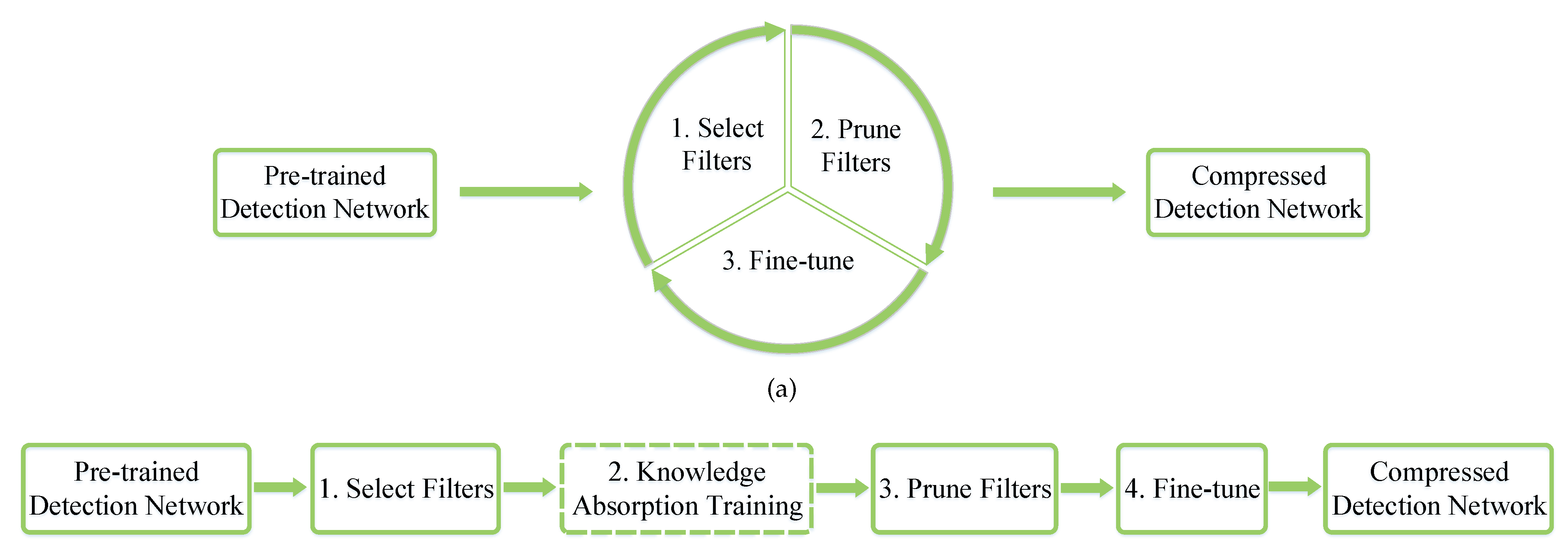
17]. Therefore, we take CenterNet as the pre-trained network for the absorption pruning method. The absorption pruning method is designed as a four-stage pruning method, as shown in
Figure 1b. First, the absorption pruning method selects filters that are easily absorbed from the pre-trained network, according to the filter selection criteria proposed in this paper. Second, the knowledge absorption training algorithm designed in this paper smoothly transfers the “knowledge” of the selected filters to the rest of the network. Third, the selected filters are removed from the network. Fourth, fine-tuning is conducted to recover the network performance. Finally, the absorption pruning method outputs a light object detection network. In this process, according to the characteristics of remote sensing objects and the characteristics of the deep neural network feature extractor, we design a pruning ratio adjustment method to allow the absorption pruning method to better adapt to the remote sensing object detection task.
The contributions of this paper can be summarized as follows:
We propose a new pruning pipeline that does not require the iterative mini-batch pruning used in the classic pruning pipeline.
The absorption pruning method provides a knowledge absorption training method, which can smoothly transfer the “knowledge” in some filters to the remaining filters.
A filter selection criterion that can identify filters that are easily absorbed is proposed.
We design a pruning ratio adjustment method based on the remote sensing object characteristics, such that absorption pruning can better facilitate remote sensing object detection network compression. To the best of our knowledge, this is the first pruning ratio adjustment method designed for remote sensing object detection network pruning, according to remote sensing object characteristics.
3. Methods
A unique pruning method for remote sensing object detection network compression is proposed in this paper. In
Section 3.1, we first introduce the overall framework of the proposed method in detail, focusing on the difference in pipeline compared to existing pruning methods. Then, the unique filter selection criterion and absorption pruning training approach are introduced in
Section 3.2 and
Section 3.3, respectively. Furthermore, a method for pruning ratio adjustment that considers object features in remote sensing imagery is proposed in
Section 3.4. Finally, we introduce the pruning strategy of pruning CenterNet in
Section 3.5.
3.1. Overall Framework
Most traditional network pruning methods adopt a classical three-stage iterative pruning pipeline, as shown in
Figure 1a. Specifically, these methods first select unimportant parameters from the network, according to the designed criteria. Then, these selected parameters are removed from the network. Finally, fine-tuning is conducted, in order to recover the performance damage caused by removing parameters. To avoid removing too many parameters at a time, which may cause irreversible damage to network performance, researchers typically choose to prune a small batch of parameters from the network each time, removing redundant network parameters by repeating the above three-stage operation many times. However, there are two significant unreasonable aspects in the classic pipeline: first, the iterative selection–pruning–fine-tuning pipeline consumes a lot of time and computing resources; second, the classic process simply removes parameters that still contain a lot of “knowledge” and then hopes to re-learn that knowledge through fine-tuning.
Therefore, the filter pruning pipeline shown in
Figure 1b is proposed in this paper in order to avoid the above two problems. The pipeline proposed in this paper also starts with a pre-trained network, but abandons the traditional three-stage iterative operation and replaces it with a four-stage operation that only needs to be performed once: filter selection, knowledge absorption training, pruning, and fine-tuning.
Different from the classical pipeline, we no longer directly remove a selected filter but design a knowledge absorption training method to smoothly transfer the “knowledge” in the selected filter to the rest of the network and then prune these filters. This process of transferring “knowledge” allows the “knowledge” to be absorbed by the rest of the network. Therefore, we call this method the knowledge absorption training method, which is also the origin of the word “absorption” in this paper. Ideally, pruning performed after the knowledge in the filter has been fully absorbed will not cause any damage to model performance; however, in practice, due to the limitations of training techniques, the knowledge in the selected filter cannot be completely absorbed, and the pruned filters still contain a small amount of knowledge. Therefore, fine-tuning is required to recover the performance damage.
3.2. Filter Selection Criteria
Classic pruning methods select filters and prune them directly; therefore, unimportant filters should be selected to avoid a significant drop in network performance. However, the proposed absorption pruning method requires the rest of the network to absorb the knowledge in the selected filters, and so we need to choose easily absorbed filters. In other words, the knowledge contained in the selected filters should be easier to learn.
Assume that the parameter tensor of the
jth filter of the
ith layer of the network is
, where
c,
o,
w, and
h represent the number of input channels, the number of output channels, the width of the convolution kernels, and the height of the convolution kernels, respectively. In the process of training a complex network as a pre-trained network, the distance between the filter parameter tensor
and its final converged parameter tensor
can be defined as follows:
where
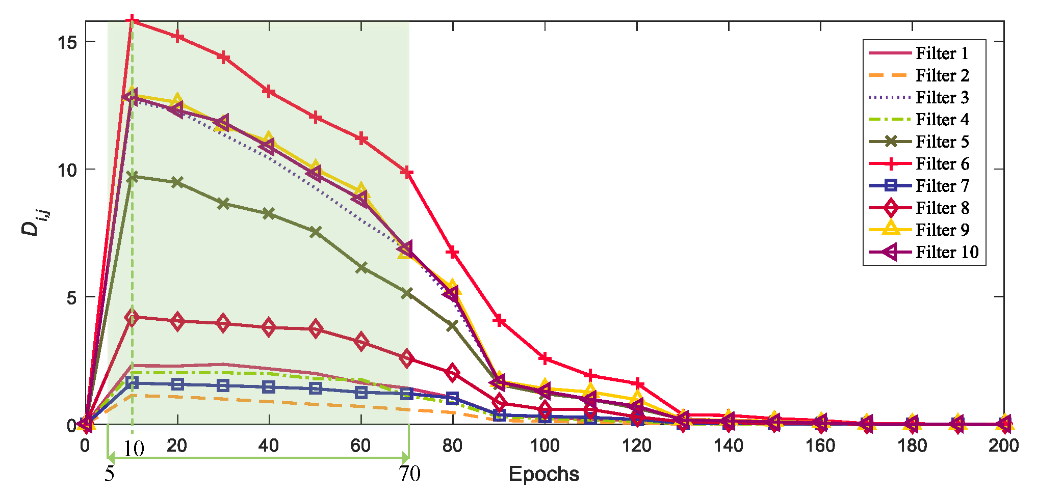
represents the L1-norm. To measure the learning difficulty of different filter parameters, we monitor the parameter change during the training of the CenterNet network for the object detection task.
Figure 2 shows the changes in the parameters of 10 randomly selected filters from CenterNet. The horizontal axis represents the training epoch, while the vertical axis represents
. Specifically, in the training process of the pre-trained network, we randomly select 10 filters as observation objects and record the parameters of these filters in different epochs. After the pre-trained network is trained to convergence, the
values of the 10 filters at different epochs are calculated, according to Equation (
1), and the final
value variation curves with epochs are plotted in
Figure 2.
Figure 2 contains two essential pieces of information: first, all filter parameters were initialized very well. The initialized filter parameters were very close to the optimized parameters (i.e., the
values of all filters are close to 0). The second is that the direction of the minimum gradient of the filter parameters during the training process was not consistent with the direction of the shortest distance (the lower curve is closer to the shortest distance than the upper curve). Therefore, we realized that this phenomenon can be used to measure the learning difficulty of filter parameters in order to construct a simple and unique filter selection criterion. Specifically, only the model at a certain stage and the final model need to be stored. Then, the value of
for each filter is obtained according to Equation (
1). A larger
indicates that the filter
is more challenging to learn. In addition, it can be seen, from
Figure 2, that when the epoch is within the interval (5, 70), the convergence distance curves of different filters have obvious differences and rarely cross. Thus, when training the pre-trained network, we only save the
and the final converged model parameters to evaluate the filter absorption difficulty and select the filter from the converged pre-trained network according to the absorption difficulty score.
3.3. Knowledge Absorption Training
For object detection tasks, the goal is to accurately predict the location and size of the object bounding box. Taking CenterNet as an example, the training loss function consists of three parts [
42]:
where
represents the prediction loss of the object centre,
represents the prediction loss of the width and height of the object bounding box, and
represents the bias loss of the predicted object center.
Knowledge absorption training aims to transfer the knowledge from the selected filters to the rest of the network such that the selected filters can be removed harmlessly. In the absorption pruning algorithm proposed in this paper, we design an absorption loss
to absorb the knowledge in the selected filters. Therefore, the new loss function in the absorption training is:
where
is the weight of
.
Note that is defined to disable the selected filters gradually, while , , and jointly ensure that the detection performance of the network does not decline during the process of the selected filters gradually losing their effect.
It should be noted that, in most existing convolutional neural networks, the convolutional layer is followed by a batch normalization layer to address the internal covariate shift problem [
43]:
where
represents the output of the
ith convolutional layer;
represents the output of the normalization layer after the
ith convolutional layer;
and
represent the expectation and variance of
calculated over the training set, respectively; and
and
are the scaling and offset parameters of the normalized
, respectively. The pair
and
serve as a gate for the output of a filter in the
ith convolutional layer: if both
and
are 0, then the filter parameter
will be entirely useless in the network.
Therefore, a new absorption loss is designed for gradually disabling selected filters by penalizing specific
and
combinations:
where
is a 0,1 sequence, representing the index of the selected filter of the
ith convolutional layer. An element 1 in
indicates that the corresponding filter is selected, while an element 0 indicates that the corresponding filter is not selected. It is worth mentioning that the work in [
44] used a similar loss function design to regularize the parameter
and proved its effectiveness. As such, the design of the loss function
used in this paper was inspired by the article [
44].
3.4. A Method for Pruning Ratio Adjustment Based on Remote Sensing Image Features
Compared with traditional optical images, the objects in remote sensing images have two remarkable characteristics: first, the size of the objects is tiny. This is because remote sensing imagery is usually imaged very far away from the object, and so the spatial resolution of the object is low. Second, the object features are typically very simple. For optical remote sensing imagery, this is mainly due to the long imaging distance. For SAR remote sensing imagery, in addition to the long imaging distance, it is also mainly affected by factors such as the low frequency of electromagnetic waves (compared to visible light) used by SAR imaging technology, the lack of rich color information, and strong background noise. Therefore, the objects in SAR images are only composed of a set of scattered points with different brightnesses and positions, and the provided object features are relatively simple.
In a related manner, DCNN also has two key characteristics. One is that higher convolutional layers have larger receptive fields, and the other is that the features extracted by higher convolutional layers are also more complex. Therefore, two inferences are easily drawn when DCNNs are used for object detection on remote sensing imagery. First, as the object size in the remote sensing image is small, a large receptive field is not required. Second, the features of remote-sensing objects are simple, and so the features extracted by the lower convolutional layers are more important. Based on such prior knowledge, we designed a method according to each layer’s receptive field in order to adjust the absorption pruning ratio flexibly.
Traditional network pruning methods usually adopt the same pruning ratio
in each convolution layer. Considering the characteristics of the remote sensing object and DCNN analyzed above, the absorption pruning method used for remote sensing object detection networks should remove more filters with large receptive fields and retain more filters with small receptive fields. Equations (
6) and (
7) detail the calculation methods for the receptive field:
where
represents the receptive field of the
ith convolutional layer,
is the convolution kernel size (or pooling size) of the
ith convolutional layer, and
is the convolution stride.
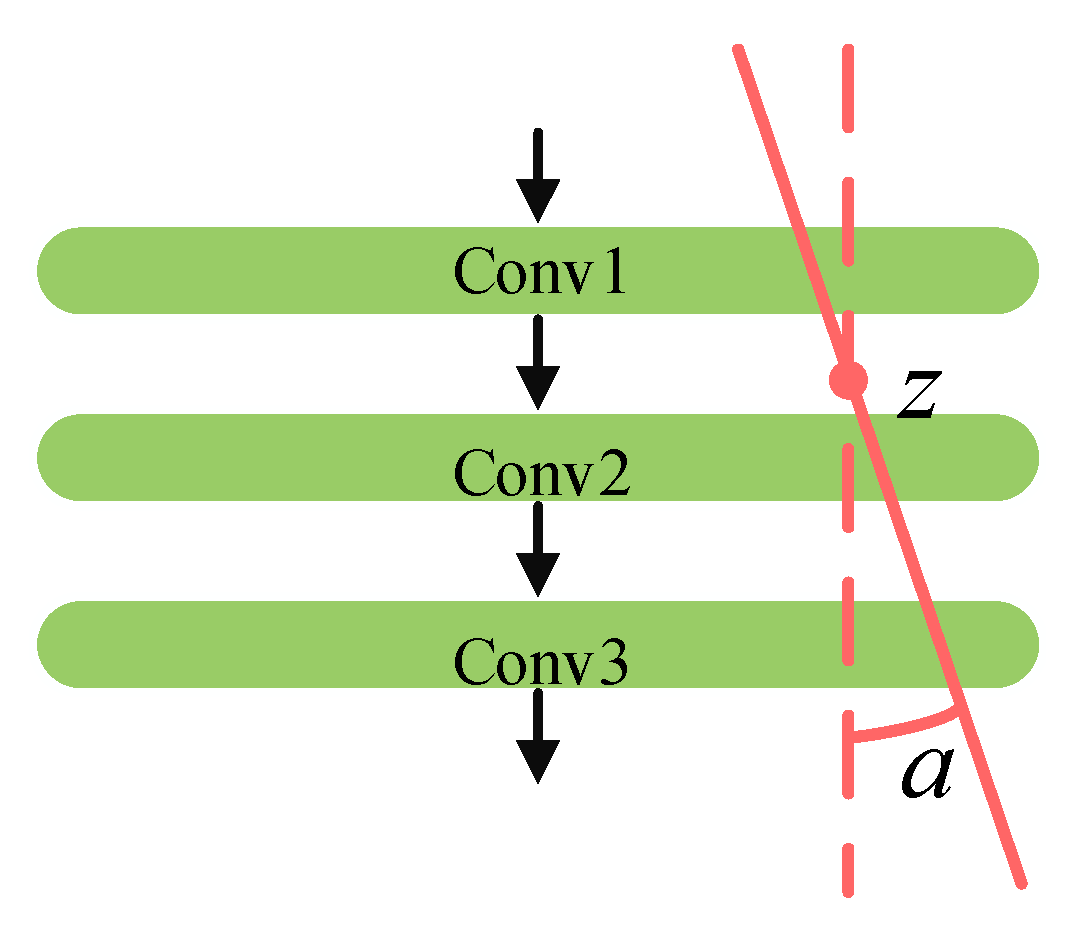
We define the adjustment factor of the pruning ratio as
and define the minimum receptive field necessary for extracting remote sensing object features as
z (i.e., the threshold to judge whether the receptive field is too large or too small). Then, the adjusted pruning ratio
for the
ith convolution layer can be calculated, according to Equation (
8).
Figure 3 illustrates the adjustment process for the pruning ratio. As shown in
Figure 3, the adjustment of the pruning ratio is similar to a “lever”, where the parameter
z controls the “fulcrum” of the lever, and the parameter
controls the adjustment range.
3.5. Pruning Strategy for CenterNet
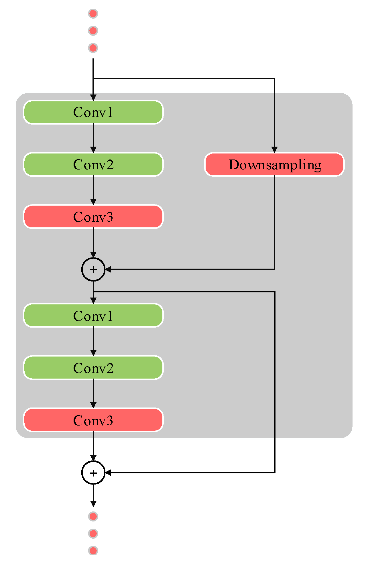
CenterNet101 uses the feature extractor of ResNet101 as the backbone of the network. ResNet uses an innovative residual structure to fuse the output features of different network layers. This innovation facilitates the excellent performance of the ResNet structure network, but the complex network structure also brings challenges for network pruning.
The ResNet structure network usually consists of multiple convolution blocks, as shown in
Figure 4. In order to avoid the trouble of pruning filters in down-sampling layers, traditional pruning algorithms usually only prune the convolution layers shown in green [
21]. The absorption pruning algorithm proposed in this paper also includes the red convolutional layers in the pruning range. The specific approach is as follows: treat the red convolutional layers in each convolutional block as a convolutional layer, and these layers share the same sequence of filter learning difficulty. In the filter selection stage, the learning difficulty score of each filter in the red layer is calculated as follows:
where
o represents the number of filters in the
ith convolutional layer, and
n represents the number of coupled convolutional layers (i.e., red convolutional layers in
Figure 4) in each convolutional block. Therefore, the filters in all red convolutional layers in each convolutional block have the same sequence of filter importance scores, and the filters with the same index in these layers will be absorbed, pruned, or retained simultaneously. The absorption pruning algorithm can also implement pruning for all layers of the CenterNet101 backbone.
The algorithm proposed in this paper is summarized as Algorithm 1:
| Algorithm 1 Detailed process of the absorption pruning method. |
Input: Pre-trained network with parameter , network with parameter when epoch = 10, training set T, pruning ratio x, absorption training epochs E Output: Lightweight network - 1:
Calculate the learning difficulty score of all filters in the pre-trained network: - 2:
Sort all training difficulty scores of the ith convolutional layer in ascending order to obtain the score set - 3:
Calculate the pruning ratio of the ith convolution layer according to Equation ( 8) - 4:
Obtain the filter score threshold , where - 5:
Select all filters with scores lower than the threshold to obtain the masks of each layer, - 6:
for; ; do - 7:
according to Equation ( 3). - 8:
- 9:
Update - 10:
Prune all selected filters. - 11:
Fine-tune to restore network performance - 12:
return
|
4. Experiments and Discussions
Experiments were carried out to verify the effectiveness of the proposed absorption pruning method. The detailed experimental settings are introduced in
Section 4.1.
Section 4.2 details the performance of the pre-trained network and the pruning results of the absorption pruning method at different pruning ratios.
Section 4.3,
Section 4.4 and
Section 4.5 describe the effectiveness verification experiments for different functional modules of the absorption pruning method. In
Section 4.6, the absorption pruning method is compared with other state-of-the-art network pruning methods in order to further verify its effectiveness. Hyperparameter selection experiments for the pruning ratio adjustment method are detailed in
Section 4.7. In addition, partial object detection visualization results of the pruned lightweight network are shown and analyzed in
Section 4.8.
4.1. Implementation Details
4.1.1. Data Sets
According to the imaging band, visible light remote sensing and SAR remote sensing are the most important means of earth observation for spaceborne or airborne platforms. In order to verify the effectiveness of the proposed absorption pruning algorithm on the object detection network in remote sensing imagery, we conducted experiments on two typical remote sensing object detection data sets: the SAR image data set SSDD [
25] and the visible light remote sensing image data set RSOD [
45].
The SSDD data set contains 1160 images and 2456 ships, with an average of 2.12 ships per image. The data are mainly from slices of RadarSar-2, TerraSAR-X, and Sentinel-1. The spatial resolution of the images is 1–15 m, and the average size of the images is
pixels.
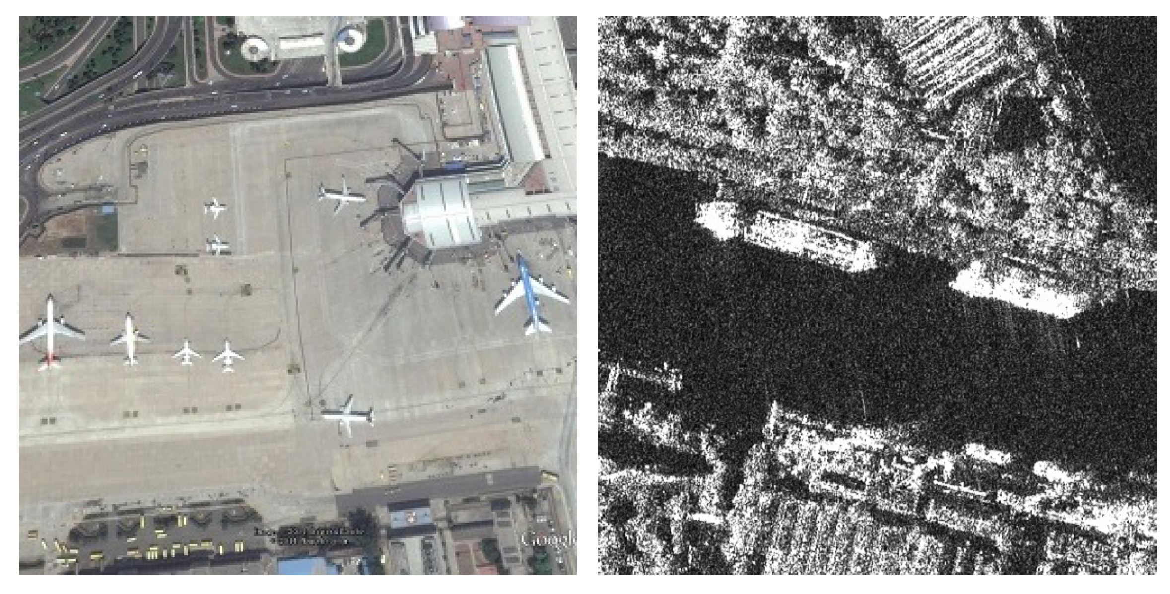
Figure 5 (Right) shows an image from the SSDD data set. Furthermore, in the experiments in this paper, the samples in the SSDD data set were randomly divided into training, test, and validation sets in a ratio of 8:1:1.
The RSOD data set was released by Wuhan University in 2015. It contains four types of objects: oil tank, aircraft, overpass, and playground. Researchers often use it as a validation data set for object detection algorithms based on optical remote sensing imagery.
Figure 5 (Left) shows an image from the RSOD data set. We mixed the four classes of samples in the RSOD data set and randomly divided them into training, test, and validation sets in a ratio of 8:1:1.
4.1.2. Pre-Training
CenterNet101 was trained from scratch on the SSDD and RSOD data sets to obtain the pre-trained networks. We used the Adam optimizer during training. In addition, the max number of training epochs was set to 200, and the initial learning rate was set to 1.25 × 10⁻⁴ and decayed by a factor of 0.1 at the 90th, 130th, and 170th epochs.
4.1.3. Absorption Training and Fine-Tuning
For absorption training, the Adam optimizer was still adopted. The total number of training epochs was set to 60, and the initial learning rate was set to 1.25 × 10⁻⁴ and decayed by 0.1 at the 30th epoch. In the fine-tuning stage, we also used the Adam optimizer and set the total number of training epochs to 60. It should be emphasized that fine-tuning usually adopts a lower learning rate. Therefore, the initial learning rate was set to 1.25 × 10⁻⁶, and was also decayed by 0.1 at the 30th epoch. It is worth noting that the total number of training epochs was set to 60 based on our observation of experimental phenomena. In other words, the selection of these hyperparameters was based on empirical evidence.
4.1.4. Other Experimental Parameter Settings
In all experiments, the sample batch size for training and testing was set to 8. The CenterNet101 network was used as the pre-trained network for all experiments. Considering the average size of images in the SSDD data set, the hyperparameter
z of the pruning ratio adjustment method employed in the experiments shown in
Section 4.4 and
Section 4.6 was set to 500, and the pruning ratio adjustment method hyperparameter
was set to 1. The weight parameter
of
in Equation (
3) was set to 1 × 10
3 for all experiments. In addition, the detection accuracy mAP used in this paper refers to mAP50.
4.2. Pre-trained Networks and Pruning Results
According to the training settings in
Section 4.1.2, we trained CenterNet101 on the SSDD and RSOD data sets to obtain the pre-trained networks. The pre-trained CenterNet101 networks achieved an mAP of 91.08% and 88.29% on the SSDD and RSOD data sets, respectively.
We input these networks into the absorption pruning method for pruning experiments with different pruning ratios. The pruning results are detailed in
Table 1. From the experimental results on the SSDD data set, when the filter pruning ratio was not more than 60%, the detection performance of the pruned CenterNet101 was significantly better than that of the pre-trained network. This was because pruning alleviated the over-parametrization problem of CenterNet101, which reduced over-fitting. In addition, even when 85% of filters were removed from the pre-trained network, the object detection accuracy of the pruned network was only 0.58% lower than that of the pre-trained network. However, the pre-trained network parameters and storage space requirements are ten times larger than those of pruned networks. These results demonstrate that the absorption pruning method can effectively compress the DCNNs in SAR ship detection.
From the experimental results on the RSOD data set, it was found that when the pruning ratio did not exceed 60%, the pruned model networks also obtained better object detection performance than the pre-trained network. When the pruning ratio was increased to 85%, the network performance significantly declined after pruning. This phenomenon indicates that, compared with the SAR object detection task on the SSDD data set, the task on the RSOD data set—containing four types of optical objects—was more complicated and required higher network complexity. The overall results demonstrated that the absorption pruning algorithm proposed in this paper can effectively compress DCNNs for optical remote sensing object detection.
4.3. Absorption Training Validation Experiment
To verify the effectiveness of the absorption training approach, we used the CenterNet101 trained on the SSDD data set as the target and selected 10% of the filters, according to the proposed filter selection criterion, for knowledge absorption training. In order to exclude the influence of other factors, the pruning ratio adjustment and fine-tuning were not enabled in this experiment.
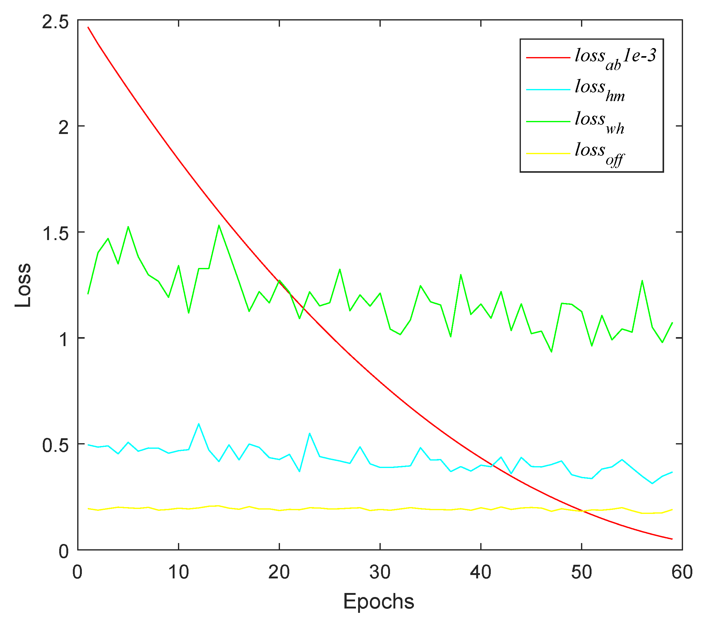
Figure 6 shows the change curves of the loss function during absorption training. According to the analysis of Equation (
3) in
Section 3.3, the
,
, and
are indicators of network detection performance, while
indicates how much the selected filters contribute to the network. As shown in
Figure 6, during the absorption training process,
decreased rapidly while
,
, and
only fluctuated within a small range. These results indicate that the selected filters rapidly lost their effect while the network performance was almost unchanged. It appears that the rest of the network absorbed the knowledge in the selected filters. It is worth mentioning that, in order to clearly show the changes in the four losses in the same figure,
was multiplied by a factor of 1 × 10
−3.
In addition,
Table 2 provides a comparison of the pruned network detection accuracy with and without absorption training under different filter pruning rates. It can be seen that the pruned networks after absorption training could retain most of the detection accuracy after pruning, while the pruned network without absorption training only retained part of the detection performance in small-scale pruning; however, when the pruning ratio was higher than 35%, the pruned network almost completely lost the ability to detect objects.
These results demonstrate that knowledge absorption training can effectively transfer the “knowledge” in the selected filter(s) to the rest of the network before pruning, thus effectively avoiding the performance damage caused by filter pruning.
4.4. Filter Selection Criteria Validation Experiment
To verify the effectiveness of the proposed filter selection criterion, we used the CenterNet101 trained on the SSDD data set as the target, and selected 10% of the filters in ascending, descending, or random order of learning difficulty for knowledge absorption training. In order to exclude the influence of other factors, the pruning ratio adjustment method and fine-tuning were not enabled in this experiment.
Absorption training on randomly selected 10% of filters was used as a benchmark. Theoretically, absorption training on the 10% filters with the lowest learning difficulty should provide the highest absorption efficiency (i.e., the contribution index
of the selected filter decreases rapidly under the premise that the object detection performance indicators
,
, and
of the network remain stable). Meanwhile, absorption training on the 10% most difficult-to-learn filters is expected to lead to the lowest efficiency. The experimental results presented in
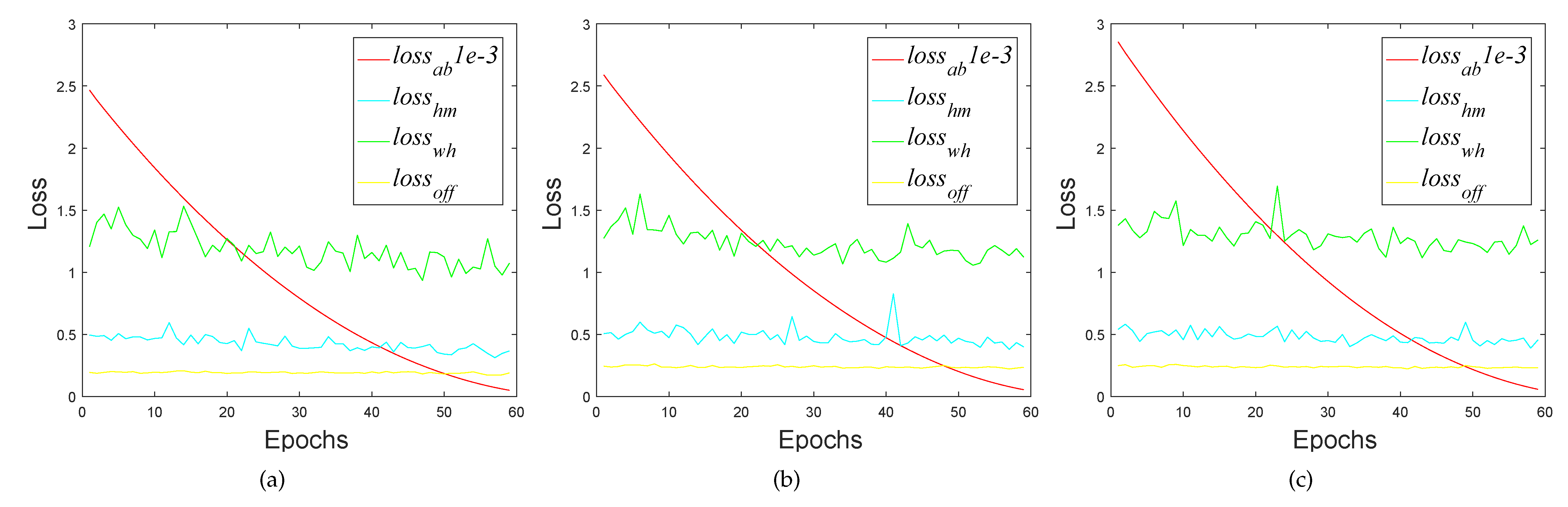
Figure 7 show that the ordering of filter learning difficulty conformed to our theoretical expectations, proving that the filter selection criterion proposed in this paper can effectively score the learning difficulty of filter parameters. In addition, it can be seen, from
Figure 7, that the
,
, and
values representing the network detection performance also showed a downward trend as the selected filters gradually lost their function during absorption training. This phenomenon indicates that the over-fitting problem of the network is gradually alleviated. Among them, the network (
Figure 7a) that conducts knowledge absorption training in ascending order of filter parameter learning difficulty obtained the highest loss reduction, the network (
Figure 7b) that conducted knowledge absorption training in random order of the difficulty of filter parameter learning was in second place, and the network (
Figure 7c) that conducted knowledge absorption training in descending order of filter parameter learning difficulty obtained the worst loss reduction. This phenomenon also demonstrates that the filter selection criteria proposed in this paper can, indeed, select the most easily absorbed filter.
In order to further verify the effectiveness of the filter selection criteria proposed in this paper, the filters of the pre-trained network were pruned in the same ratios according to the increasing, random, and descending order of parameter learning difficulty, respectively. Except for the filter selection method, the rest of the experimental settings were kept the same, and the experiment was carried out on the SSDD data set. After selecting the filters, the pre-trained network went through the process of absorption, pruning, and fine-tuning. The accuracies of the obtained lightweight detection networks are given in
Table 3.
As can be seen from
Table 3, under the condition of the same filter selection ratio, selecting the easiest-to-learn filters can provide the best lightweight network while selecting the most difficult-to-learn filters led to the worst network. These results demonstrate that the filter learning difficulty evaluation criterion proposed in this paper is reasonable.
4.5. Pruning Ratio Adjustment Method Validation Experiment
Experiments were also carried out to verify the effectiveness of the proposed pruning ratio adjustment method. The CenterNet101 trained on the SSDD data set was again used as the test object. The pre-trained CenterNet101 underwent absorption training, pruning, and fine-tuning with and without the pruning ratio adjustment method, and finally, lightweight compressed networks were obtained.
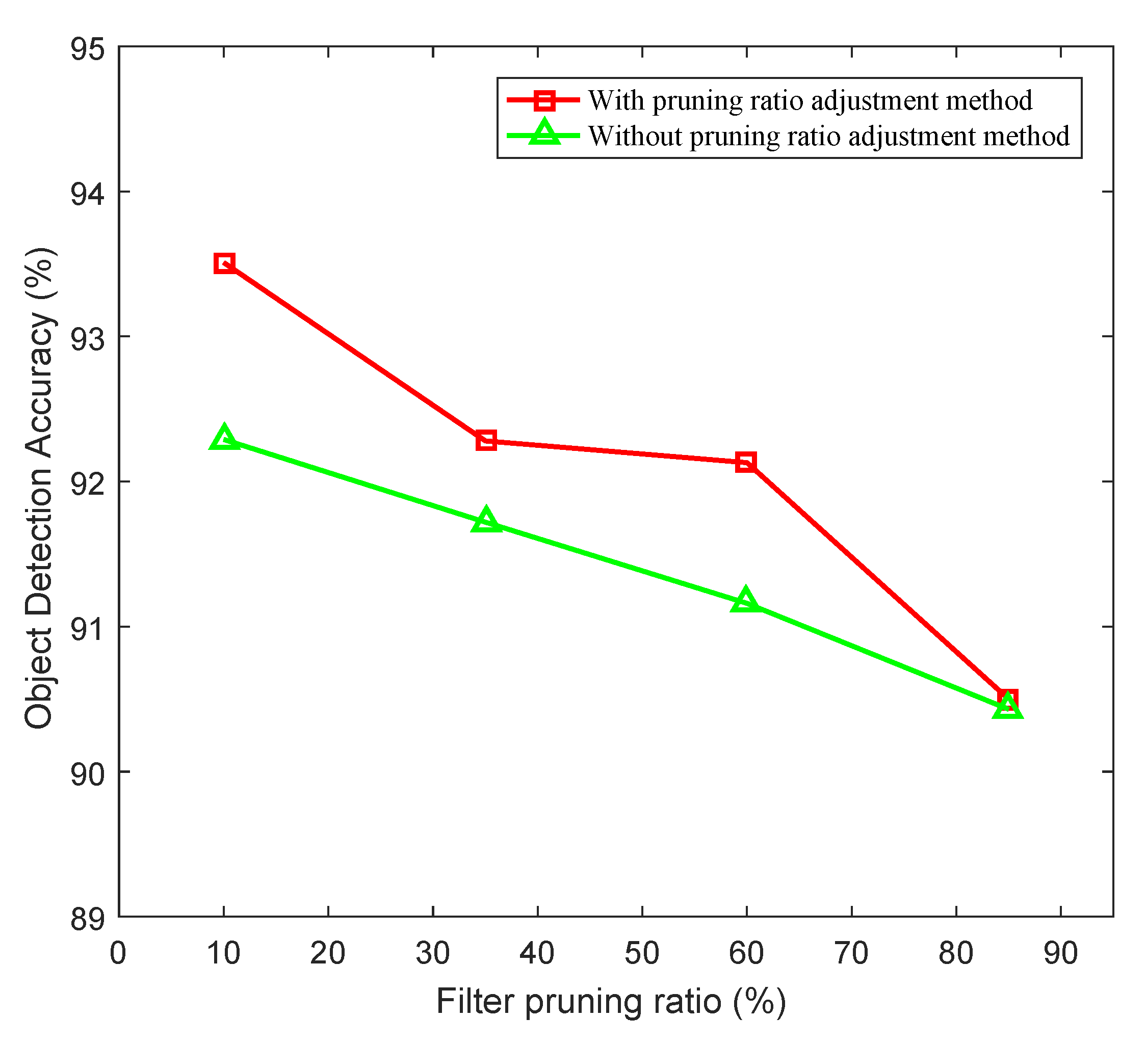
Figure 8 depicts the performance of the compressed networks with and without the pruning ratio adjustment method at different pruning ratios. It can be seen that the pruning ratio adjustment method specially designed for remote sensing image object detection enhanced the absorption pruning method. By analyzing the number of filters in each layer of the compressed networks obtained with and without absorption pruning, we observed that the method for the pruning ratio adjustment proposed in this paper can, indeed, help absorption pruning to focus on pruning top convolutional layers and reduce the pruning of bottom convolutional layers.
4.6. Comparison with Other Pruning Methods
To further verify the effectiveness of the absorption pruning method proposed in this paper, four network pruning methods were used to prune CenterNet101 for remote sensing object detection: the classic pruning method L1 [
14], APoZ [
15], Taylor [
16], and the state-of-the-art (SOTA) pruning method HRank [
12]. Under the same pruning rate, L1, APoZ, Taylor, and HRank adopt the classic pruning pipeline to prune filters in a layer-by-layer manner. In this process, L1, APoZ, Taylor, and HRank uniformly pruned eight times and fine-tuned for 30 epochs after each pruning to restore network performance.
The detailed experimental results are shown in
Table 4. It can be seen that the performance of the absorption pruning method proposed in this paper was better than that of the SOTA method and significantly better than those of the classic pruning methods. Moreover, as L1, APoZ, Taylor, and HRank were designed for pruning optical object classification networks, they perform worse than expected in remote sensing object detection network compression tasks. These results demonstrate that the absorption pruning method proposed in this paper is more suitable for the network compression task of remote sensing object detection and can achieve SOTA performance.
4.7. Hyperparameter Experiment for Proposed Pruning Ratio Adjustment Method
In order to explore the influence of the values in the hyperparameter combination of
z and
on the absorption pruning method, we fixed the pruning ratio as 60% and conducted experiments on both the SSDD and RSOD data sets. From the experimental results shown in
Table 5, it can be seen that the absorption pruning method performed better when the pruning ratio adjustment magnitude
was five. A too-small value of
cannot take full advantage of the pruning ratio adjustment method, while an excessively large
will degrade the network performance. When the pruning ratio adjustment fulcrum
z was 300, it was obviously better than when
z was 500 and 700. This indicates that, in the object detection task on remote sensing images, the lightweight network should retain more filters with a receptive field below 300 while removing more filters with a receptive field greater than 300. Considering that the input size of the CenterNet101 network is 512 × 512, the size of objects in remote sensing images usually does not exceed 300 × 300. Therefore, filters with receptive fields exceeding 300 are unnecessary in remote sensing object detection networks. This phenomenon is consistent with our analysis in
Section 3.4 regarding the small size and simple features of remote sensing objects.
4.8. Detection Results of the Pruned CenterNet101
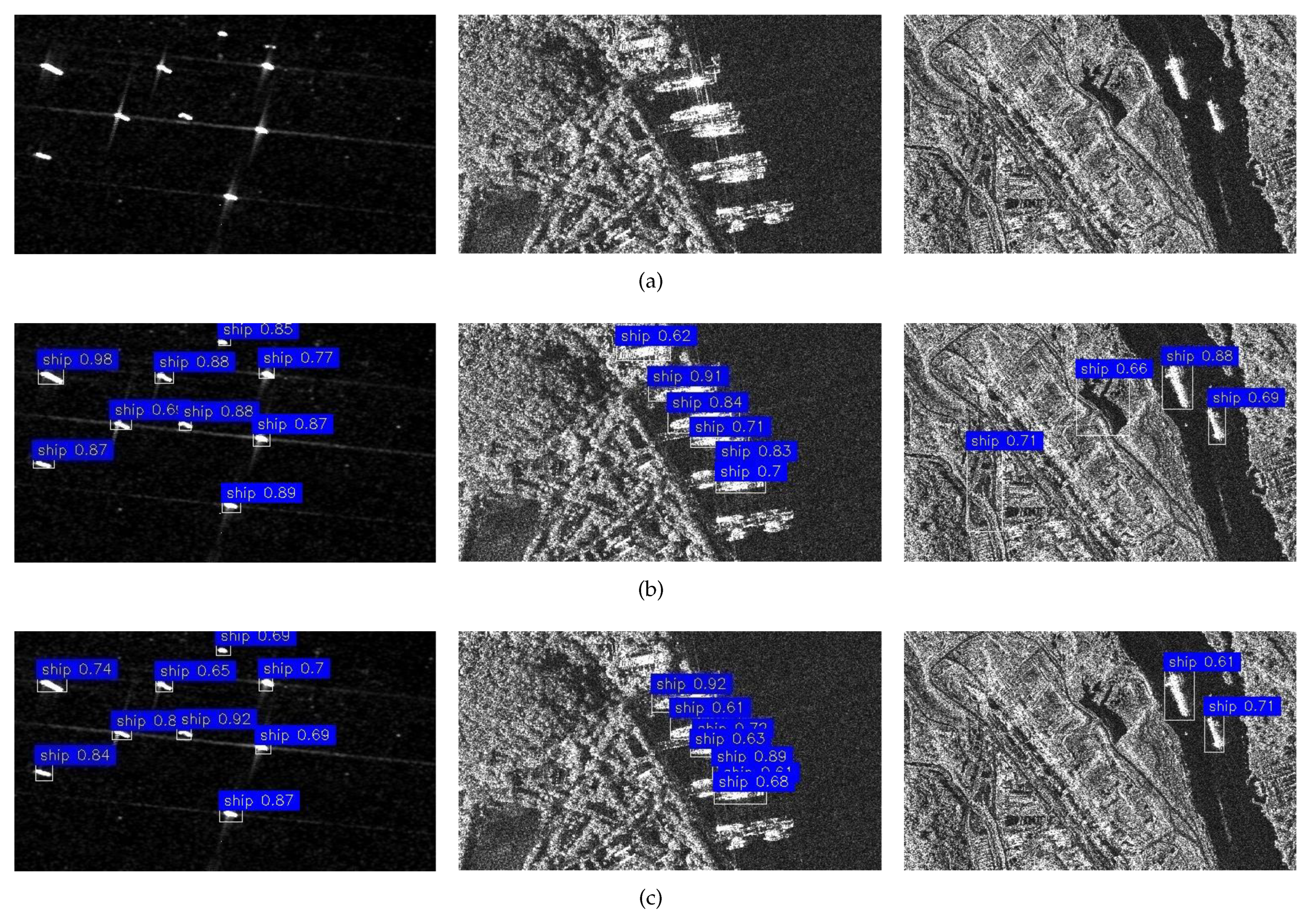
To verify the effectiveness of the absorption pruning method proposed in this paper in eliminating the over-fitting problem, we compared the object detection results of the lightweight network with 60% of filters pruned against the pre-trained network.
Figure 9 and
Figure 10 show the visualized comparison results. As seen from the left image of
Figure 9b, the pre-trained network presented very good detection performance with a pure sea surface background. In the middle image of
Figure 9b, it can be seen that the pre-trained network had misdetection (only five out of seven ships are detected) and false alarm (the lines on land are wrongly detected as a ship) problems in the dense near-shore ship detection scenario. The right image of
Figure 9b shows that the pre-trained network incorrectly detected lakes and lines on land as ships. A similar phenomenon can also be observed in
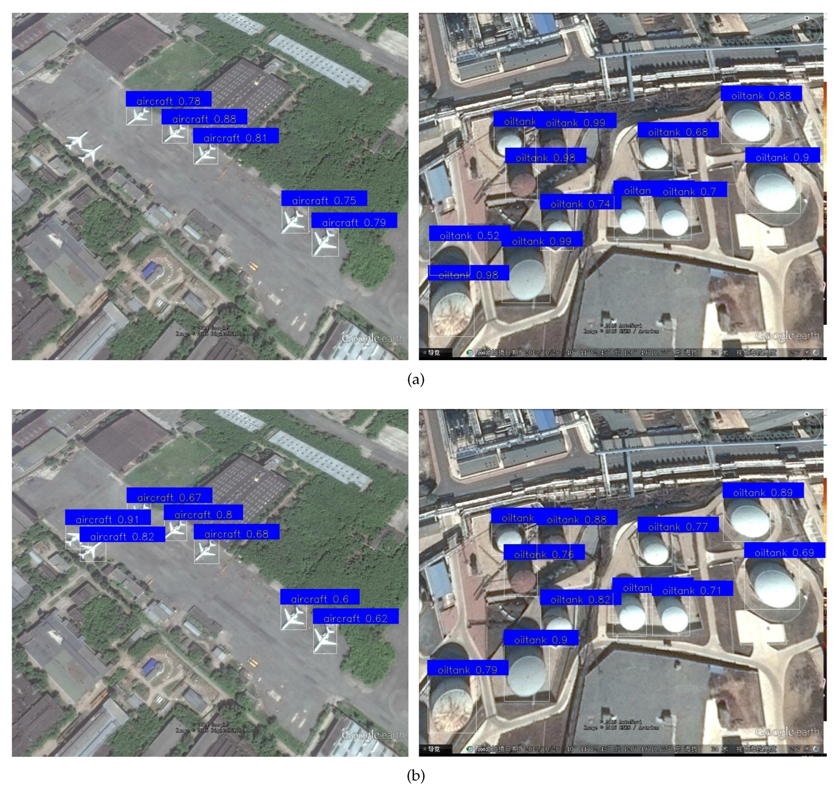
Figure 10a, where the pre-trained network failed to detect two closely aligned aircraft and wrongly detected the shadow of an oil tank as the oil tank. However, it can be seen from
Figure 9c and
Figure 10b that the lightweight detection networks avoided all of the above problems and successfully completed the object detection tasks in different complex scenes. These results prove that the absorption pruning method proposed in this paper not only can retain the detection ability of the pre-trained network but also effectively alleviates the over-fitting problem of the pre-trained network.
5. Conclusions
In this paper, we proposed a filter pruning method specifically for object detection networks in remote sensing imagery. Unlike the classical iterative pruning pipeline used by existing pruning methods, we innovatively proposed a four-step pruning pipeline that only needs to be executed once. Considering the particularity of the proposed pruning pipeline, we designed a criterion for the selection of filters that are easy to learn rather than selecting unimportant filters, as in existing pruning methods. In addition, we innovatively proposed a pruning ratio adjustment method based on the object characteristics in remote sensing images in order to optimize the design of the pruning method. The experimental results of the absorption pruning method on the SSDD data set indicated that the parameters of the pruned network were less than 10% of that in the pre-trained network, while the object detection accuracy was only reduced by 0.58%. In addition, on both the SSDD and RSOD data sets, the network performance was improved by more than 1% after the absorption pruning method removed 60% of the filters from the pre-trained network. These results demonstrate that the proposed absorption pruning method can effectively remove the redundant parameters in the remote sensing object detection network, thus eliminating the over-fitting problem.


