Design of f-SCAN Acquisition Mode for Synthetic Aperture Radar

Abstract

This paper presents the design and processing of the SAR acquisition technique named frequency scanning (f-SCAN), aimed to obtain high sensitivity to targets with low backscattering and to improve the signal-to-noise ratio (SNR) in wide-swath systems. The f-SCAN is an interesting alternative to the scanning on receive method (SCORE), which needs multiple phase centres achieved using the digital beam forming (DBF) technique. f-SCAN requires less hardware complexity than SCORE; at the same time, it improves the sidelobes and ambiguities’ suppression. The elements used in f-SCAN to generate the pencil beam are the true time delay lines (TTDLs) and the phase shifters (PSs). The general methodology to design an f-SCAN spaceborne SAR high-resolution wide-swath (HRWS) system is introduced; emphasis is put on the mathematical definition of the timing parameters and on a novel method of using TTDLs to achieve the full spanning of wide swaths. The processing of f-SCAN data is also considered: we introduce a novel algorithm to limit the data volume and to guarantee an almost invariant slant range impulse response function (IRF) by removing spectral distortions. Eventually, new definitions, specific for f-SCAN, of the well-known SAR performance parameters, are provided. Simulation results and performances are presented. The advantages and disadvantages with respect to SCORE are discussed using the design of a real case system.

1. Introduction

Synthetic aperture radar (SAR) comprises active microwave antennas mounted on airborne or spaceborne platforms that can achieve high-resolution images of the illuminated area regardless of an external source and weather conditions. They have been used for more than forty years in different space missions to monitor natural and anthropogenic phenomena: earthquakes, landslides, forest growth, desertification, glacier and sea-ice state, urban development, agriculture extension, deforestation, and many other applications [1].

With the increasing number of applications, two major requirements arose from SAR users: higher-resolution images and, at the same time, a wider swath [2,3,4]. Indeed, we passed from the 30 × 25 m² resolution in the 100 km of the swath of the ERS-1 satellite (launched in 1991) to the 5 × 20 m² resolution on the 250 km of swath in the still-operative Sentinel-1, with an improvement of 6- and 1.25-times in range and azimuth resolutions and 2.5-times in the swath width.

The contrast between the two requirements lies in the need to reduce the pulse repetition frequency (PRF) to allow the signal from a wider swath to be received, with the need to increase the PRF to allow a wider azimuth bandwidth (and so, a higher resolution) to be achieved without ambiguities [5,6].

In new-generation systems such as ROSE-L and Sentinel-1 Next Generation [7,8], a high azimuth resolution and low ambiguities are achieved by the use of multiple channels, i.e., multiple sampling during acquisition, and on-ground reconstruction of the full azimuth spectrum in the N-times PRF non-ambiguous interval. This is the well-known multiple aperture processing scheme (MAPS) technique, widely discussed in [2,9,10,11,12,13].

A high range of resolutionsis commonly achieved by increasing the range bandwidth, a resource usually not expensive in SAR systems, apart from the increase of captured noise. However, imaging a wide swath poses another problem: often, the antenna beam in elevation is too narrow to illuminate the complete swath. This brings a reduced directivity typically at swath borders and, so, the degradation of sensitivity.

Among the solutions recently proposed to overcome this limitation, we recall SweepSAR [14] and SCORE [15]. Both techniques illuminate the entire swath upon transmission, whilst, upon receiving, a high-directivity pencil beam scans the swath, tracking the locus of the return echo. SweepSAR is based on an analogue beam steering network; SCORE is instead a digital beam forming (DBF) method based on multiple receivers in elevation, each with its own digitized receiving chain. In SCORE, the wide transmit beam is generated by the full antenna height by a proper excitation of the amplitudes and phases of sub-array elements of the phased array antenna [16]. In reception, $N_{ch}$ broader beams are used by grouping subsets of sub-arrays in elevation. These beams are onboard composed to obtain an equivalent narrow beam pointing in the current position of the receiving echo. The notable element of this technique is that the composition is performed in the digital domain, so that the narrow beam can be steered at the time of the receiving echo, i.e., in the order of microseconds. SCORE then allows the directivity to remain close to its maximum value throughout the swath length. This way, the sensitivity is optimized to its highest achievable value.

A recent upcoming alternative to SCORE is represented by the frequency scanning principle. The frequency scanning principle was firstly presented in [17,18] (Airbus owns also a patent on this method). f-SCAN is based on the idea of obtaining the same advantages of the SCORE technique, but using fewer demanding electronics. The SCORE technique requires: (i) the independent acquisition and digitization of $N_{ch}$ channels and (ii) an onboard recombining network whose coefficients must change according to the fast time sampling frequency. In f-SCAN, the same result is achieved by using phase shifters (PSs) and true time delay lines (TTDLs) on the phased array antenna. Since the beam composition is completely analogous, there is no need to maintain multiple channels and, then, multiple samplers, ADCs, and so on.

The opposite of SCORE, the pencil beam is generated in both TX and RX and always using the whole antenna. The pulse transmission is performed as in a conventional SAR system, but the frequency dispersion is fruitfully exploited to gather different parts of the transmitted chirp (which indeed correspond to different frequencies) at different ground ranges. The design of the frequency rate of the pulse (i.e., an “up” or “down” chirp) is performed in such a way that, for the chirp’s frequency transmitted at first, the pencil beam must point at the far range; conversely, for the last transmitted frequencies, the pencil beam must point at near range. The same principle is valid also for the received echoes. A consequence is that the received signal is shorter than what is expected from geometry, due to the directional filter operated by the TX and RX beams.

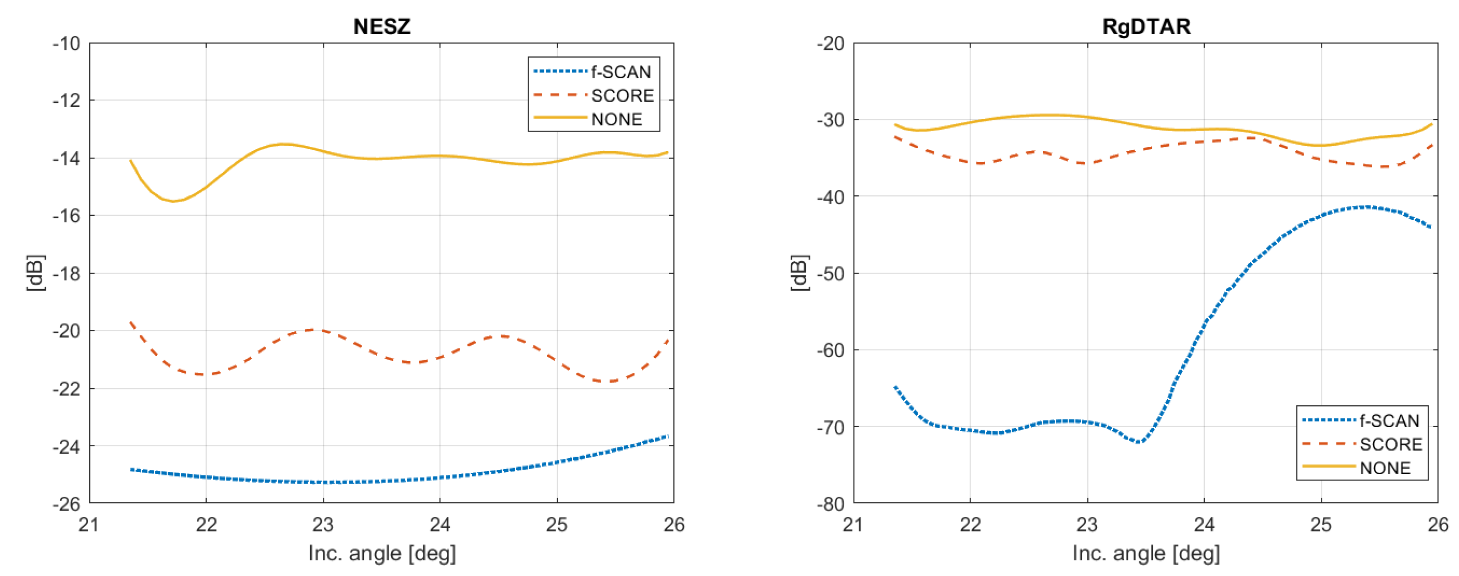
Thanks to the narrow beam used for scanning, both the transmit and receive beams have higher directivity, which means a better noise equivalent sigma zero (NESZ) and better range-distributed target-to-ambiguity ratio (RgDTAR). As will be shown, the main drawback of this method is that f-SCAN requires a larger bandwidth in transmission and a higher duty cycle.

In the recent literature, the principle of frequency scanning and frequency dispersion have been addressed. In [19,20], the concept of the conventional SCORE was extended to wide-pulse systems by proposing digital scalloped beam forming. This method has been revealed to be an effective method to soften the influence of frequency dispersion (which indeed is still interpreted as an unwanted effect) in DBF SAR. A similar result was achieved also in [21]. In [22], a novel SAR operational mode named the multi-frequency sub-pulse (MFSP) was presented: the wide-pulse bandwidth was exploited to increase the imaged swath extension without the emergence of range ambiguities. References [23,24] gave a detailed description of the implementation of the frequency scanning principle with a particular focus on the antenna, but the analysis of the corresponding SAR image capability was missing. Again, in the papers [17,18] by Roemer, where the f-SCAN principle was applied to SAR for the first time, there was not yet an exhaustive characterization of the constraints to be considered while designing a system. Moreover, the evaluation of SAR performance was only quickly introduced. In the more recent paper by Scheiber et al. [25], the focus was on the transmit pulse chirp length, which was interpreted as a trade-off parameter: the consequences on the echo window length and the benefits of dedicated onboard processing for data volume reduction were discussed. Eventually, in [26], a further version of the f-SCAN SAR, named elevation frequency scanning synthetic aperture radar (EF-SCAN SAR), was presented. In this work, the analytic space–time signal model of an intrapulse frequency scanning array was derived. Based on this, an imaging algorithm for EF-SCAN SAR was developed.

In this paper, a detailed general methodology to design an f-SCAN acquisition system is presented, giving more details than in the existing literature in the previous paragraph. The design was applied in the case of an exemplary demanding X-band spaceborne SAR acquisition mode. The processing of f-SCAN data was addressed by presenting a novel (to the authors’ knowledge) algorithm that aimed to guarantee an invariant IRF throughout the swath by removing spectral distortions. The definitions of NESZ and RgDTAR were accordingly updated. Eventually, a numerical simulation was implemented to estimate the performance figures: IRF resolution, peak and integrated sidelobe ratios (PSLR, ISLR), NESZ, and RgDTAR.

The paper is organized as follows. In Section 2, the frequency dispersion concept and the f-SCAN system and its design are explained. In Section 3, the f-SCAN processing is described, while in Section 4, the simulation results of a case study are shown and discussed. In Section 5 the theoretical performances of the f-SCAN method are defined and compared to a reference system. Eventually, conclusions in Section 6 close the paper.

2. f-SCAN System and Design

In the present section, the description of the f-SCAN principle and the main design parameters and constraints are defined. The section is organized as follows: Section 2.1 introduces the frequency dispersion principle; Section 2.2 describes how to realize f-SCAN, with particular attention to the TTDL; in Section 2.3, the definition of the elevation pattern is provided; in Section 2.4, the timing of the instrument is characterized; in Section 2.5, the conditions for data sub-sampling are derived.

2.1. The Frequency Dispersion Principle

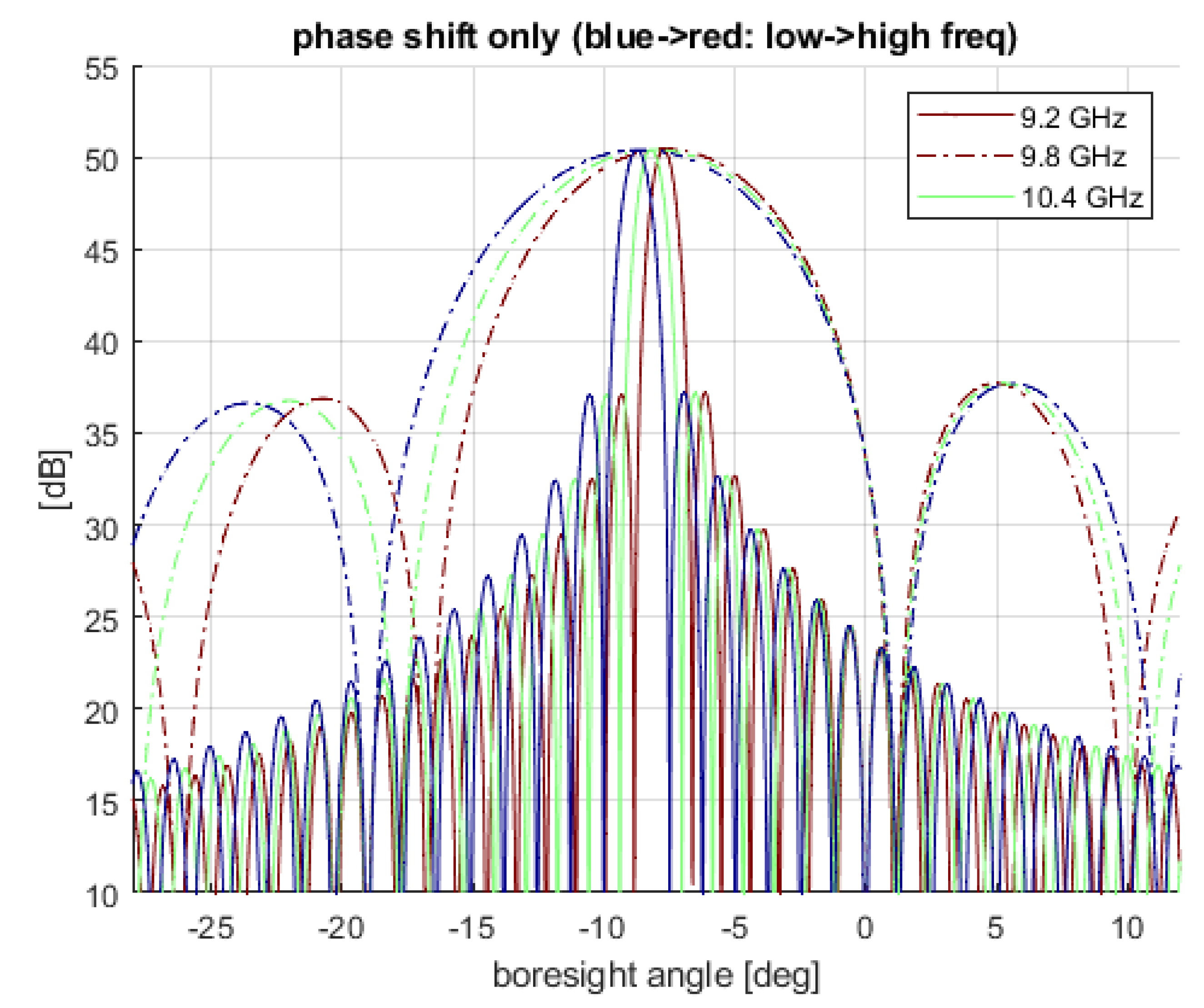
A common method to achieve the antenna pattern shape and proper steering is by using complex coefficients for the excitation of the radiating elements of an array, in both TX and RX. The embedded patterns generated by the radiating elements are usually a function of the elements’ characteristics (geometry, size, frequency), but are quite large due to their limited size. The scan direction $\theta$ of a linear array is related to a phase increment $\varphi$ introduced in the excitation coefficients used for the different elements by the following relation [16]:

$$\varphi =\frac{2\pi f}{c}sin\theta ·\Delta y$$

(1)

where f is the frequency of the signal, $\Delta y$ the distance between the elements of the array, and c the e.m. speed.

For wide-band emitted signals, however, the same phase shift $\varphi$ generates different scan directions of the array factor since the phase shift and direction coincide only for a single frequency. In practice, for a monochromatic signal, $x\left(t\right)=sin\left(2\pi f_{0}t\right)$, applying a delay or a phase produces the same effect: $x(t-t_0)=sin\left(2\pi f_0(t-t_0)\right)$ and $x(t-t_0)=sin(2\pi f_{0}t+\varphi )$, where $\varphi =-2\pi f_0{t}_0$. For a non-monochromatic signal, the application of a constant phase shift will produce different delays at different frequencies. This effect is known as frequency dispersion [16]. In Figure 1, an example of frequency shift due to the use of phase shifters only at different frequencies is shown. The modulation effect of the directivity is due to the embedded pattern of the single element.

In radar technology, a slight scanning effect of frequency is a well-known (and unwanted) problem for wide-band signals where phase shifters are used as an approximation of the (true) delay lines [17].

The frequency dispersion effect can be used as an advantage in the f-SCAN phase arrays. The basic idea is to introduce in the phase increment of the array contribution (i.e., in Equation (1) a delay line of amount $\Delta \tau$ [17]:

$$\varphi =2\pi f\Delta \tau -\frac{2\pi f}{c}sin\theta ·\Delta y$$

(2)

If the previous relation is written as a function of the scan direction $\theta$ [17]:

$$sin\theta =\frac{c}{\Delta y}\left(\Delta \tau -\frac{\varphi }{2\pi f}\right)$$

(3)

The scan direction $\theta$ results in a function of two contributions: (i) a frequency-independent term, which is commanded by a true delay increment, and (ii) a frequency-dependent term, commanded by the phase shifter.

In f-SCAN, the two degrees of freedom, i.e., the delay and the phase shifter, are used together to obtain the desired frequency dispersion. In detail:

• The phase shifter is used to steer the array factor toward the desired angle, i.e., the off-nadir centre of the swath for a SAR system. The resulting frequency dispersion of the peak is computed accordingly.
• The delay lines produce a non-dispersive shift of the peak, but also a stretching of the pattern (because of the bandwidth of the pulse), which actually results in a frequency dispersion on the grating lobe. This unwanted effect is used to complete the frequency dispersion caused by the phase shifters so as to cover the whole angular interval of the swath.

In the following section, the combined effect of the two is detailed.

2.2. Design of Phase Shifters and Delay Lines in f-SCAN

Let us design a SAR acquisition mode in which a swath with central off-nadir angle ${\theta }_0$ and width $\Delta \theta ={\theta }_{far,swath}-{\theta }_{near,swath}$ must be fully scanned in both TX and RX by a pencil beam. Let us also assume a planar array antenna with the following characteristics:

• $L_{el}$ is the elevation size (i.e., height) of the whole array antenna.
• N is the number of elements along the elevation.
• $N_{TDL}$ is the number of TTDLs. Then, the N elements from the whole antenna are grouped into $N_{TDL}$ sub-arrays of $N/N_{TDL}$ elements each.

According to the first point of the strategy, defined at the end of the previous section, the phase shift ${\varphi }_{ps}$ was designed to provide an illumination towards the swath centre ${\theta }_0$ at the carrier frequency $f_c$. The relation between ${\varphi }_{ps}$ and ${\theta }_0$, already given in Equation (1), is here repeated [16]:

$${\varphi }_{ps}=\frac{2\pi f_c}{c}sin{\theta }_0·\Delta y$$

(4)

Due to the finite bandwidth of the signal, $B_{ch}$, the corresponding frequency dispersion is given by inverting Equation (4) with the chirp frequency edges:

$$\begin{array}{cc}\hfill \Delta {\theta }_{ps}=& {sin}^{-1}\left(\frac{f_c}{f_c-B_{ch}/2}·sin{\theta }_0\right)-{sin}^{-1}\left(\frac{f_c}{f_c+B_{ch}/2}·sin{\theta }_0\right)\hfill \end{array}$$

(5)

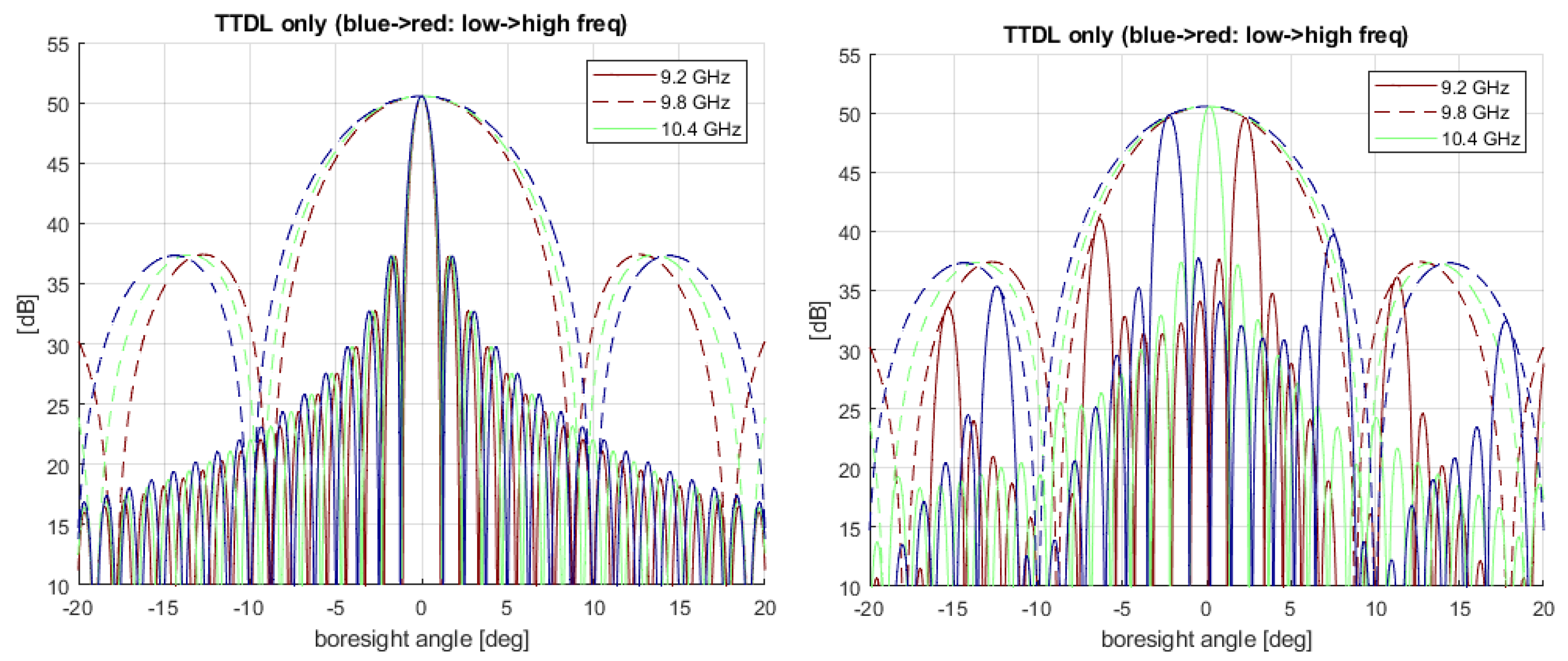
Usually, the angle interval $\Delta {\theta }_{ps}$ does not coincide with the swath angular extension $\Delta \theta$, which is dictated by other design considerations (if it coincides or is greater, this means that there is no need for further dispersion, and then, the TTDLs are useless).

For this reason, according to Step 2 of the strategy defined in Section 2.1, a set of true time delay lines was designed to achieve the full coverage of the swath. The TTDLs do not create mispointing on the main lobe, but create a frequency dispersion on the grating lobes because of the stretching of the angle axis (see Figure 2, left panel). The position of the first grating lobe depends on the wavelength $\lambda$. It is derived from the expression of the periodic sinc representing the array factor of the array antenna [16]:

$$\begin{array}{cc}\hfill F\left(\theta \right)=& \frac{sin\left(\pi \frac{L_{el}}{\lambda }sin\theta \right)}{sin\left(\pi \frac{L_{el}/N_{TDL}}{\lambda }sin\theta \right)}\hfill \\ \hfill {\theta }_{grlobe,1}=& {sin}^{-1}\left(\frac{{\lambda }_c}{L_{el}/N_{TDL}}\right)\approx \frac{{\lambda }_c}{L_{el}/N_{TDL}}\hfill \end{array}$$

(6)

where we recall that $L_{el}$ is the antenna height and $N_{TDL}$ is the number of available delay lines.

The frequency dispersion at the k-th grating lobe is then:

$$\begin{array}{cc}\hfill \Delta {\theta }_{grlobe,k}=& {sin}^{-1}\left(k·\frac{{\lambda }_{max}}{L_{el}/N_{TDL}}\right)-{sin}^{-1}\left(k·\frac{{\lambda }_{min}}{L_{el}/N_{TDL}}\right)\approx k·\frac{\Delta \lambda }{L_{el}/N_{TDL}}\hfill \end{array}$$

(7)

Please note that the previous approximation is valid until the quantities in the inverse sine are little. The frequency dispersion is then larger for farther grating lobes (i.e., the higher k, the larger the dispersion), as shown in Figure 2, right panel.

The angular interval of the swath not covered by the frequency dispersion due to the phase shifters (see Equation (5)) is covered by the stretching effect due to the use of delay lines (see Equation (7)). A good approximation of the integer number of grating lobes to be shifted is (for the exact relation, please refer to Appendix A):

$$k\approx round\left(\frac{\Delta \theta -\Delta {\theta }_{ps}}{\Delta {\theta }_{grlobe,1}}\right)$$

(8)

Eventually, the delay for each line is derived by combining Equations (3), (6), and (8):

$$\Delta \tau =\frac{\Delta Y}{c}k·\frac{{\lambda }_c}{L_{el}/N_{TDL}}$$

(9)

In Equations (9), $\Delta Y$ is the distance between the phase centre of the group of radiating elements, which share the same delay line.

2.3. Generation of the Elevation Pattern

The elevation pattern of the phased array antenna and due to phase shifters and delay lines is [16]:

$$\begin{array}{cc}\hfill {\mathrm{\Theta }}_{el}\left(\varphi \right)=& {\displaystyle {\mathrm{\Theta }}_{emb}\left(\varphi \right)\sum _{m=0}^{K-1}exp\left(-j2\pi f_c\Delta \tau ·m\right)}\hfill \\ \hfill & {\displaystyle \sum _{l=0}^{N/K-1}exp\left(-j\frac{2\pi }{\lambda }(\frac{N}{K}m+l)\Delta Y_k·sin\varphi \right)·}\hfill \\ \hfill & exp\left(-j(\frac{N}{K}m+l){\varphi }_{ps}\right)\hfill \end{array}$$

(10)

In the previous equation, $K=N_{TDL}$, ${\mathrm{\Theta }}_{emb}\left(\varphi \right)$ is the common embedded pattern from each radiating element, while $\lambda =c/f$ is the variable wavelength.

The number of delay lines is a critical design parameter and may also represent a constraint coming from the hardware. If the number of available delay lines is reduced (i.e., $N_{TDL}$ decreases), then:

• The angular position of the grating lobes (${\theta }_{grlobe,1}$) comes closer to the main lobe, as comes from Equation (6), and also, their dispersion becomes smaller. This means that the integer number of the grating lobes must increase to achieve the same angular dispersion required in Equation (8). Increasing k means a higher value of the delay, which impacts its hardware implementation.
• With fewer TTDLs, the sub-array composed pattern is narrower and the corresponding attenuation around the grating lobe is stronger. This may jeopardize the performances (e.g., NESZ) at the edge of the swath.

In Figure 3, there is a detail of the patterns in two cases, using 8 or using 4 delay lines. In the first case, the second grating lobe was used, while the fourth grating lobe was used in the second case. Even the amount of delay doubled, passing from 0.205 ns to 0.409 ns for the specific example, which shall be detailed in Section 4.

2.4. Relation between Chirp and Timing

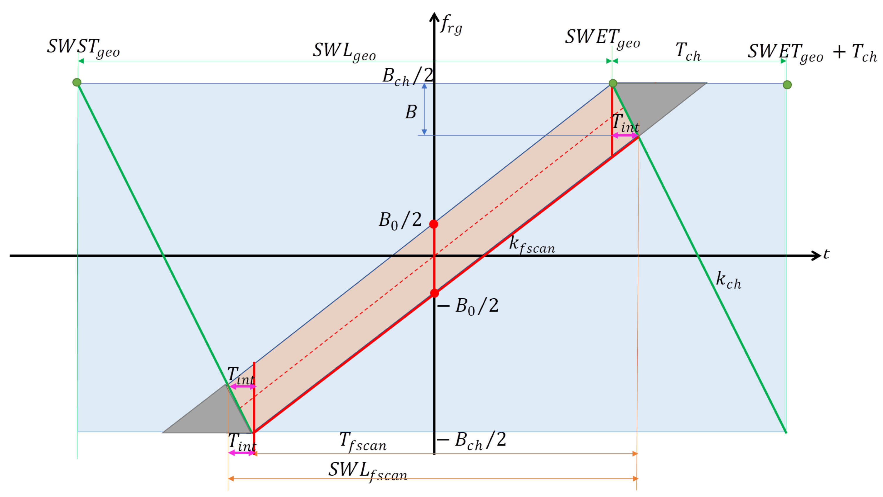
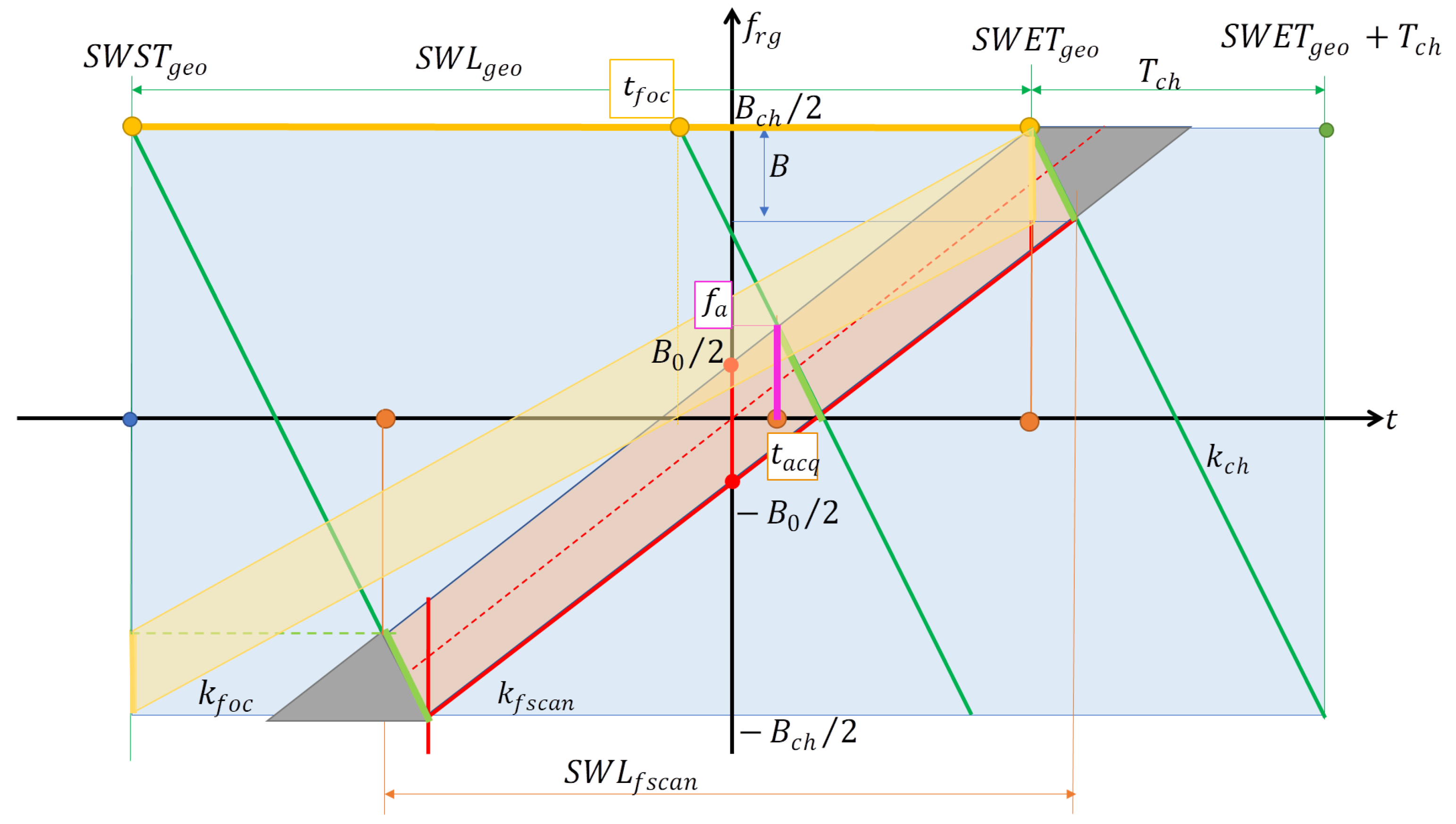
While the chirp is being transmitted, the pencil beam scans the swath so as to illuminate mainly a given portion of the underneath area. This means that each target in the swath shall be (mainly) illuminated only by a part of the chirp. This useful part of the chirp is driven by the desired range resolution of the system and is shaped, in the frequency domain, by the scanning pencil beam of f-SCAN. The principle can be effectively described using a time–frequency diagram (T-F), as the one commonly used for the slow-time Doppler relation in azimuth, with the difference that, now, it is applied to the fast time and range frequency.

To describe the f-SCAN acquisition in such diagrams, we refer to Figure 4. We assumed a chirp pulse of duration $T_{ch}$ and total bandwidth $B_{ch}$. Indeed, these parameters are often fixed by the SAR system electronics and mode design (e.g., PRF). The chirp rate is the ratio between the total bandwidth and the chirp duration: $k_{ch}=B_{ch}/T_{ch}$. In the T-F diagram, the chirp signal is represented by the green lines with a negative slope (a down chirp was assumed).

The scanning beam is instead illustrated by the reddish strip with positive slope $k_{fscan}$ and duration $T_{fscan}$. Its width, $B_0$, is the beam width in the frequency domain.

On the other hand, the geometric range resolution is a user requirement that determines the band B. The relation between $B_{ch}$ and B is illustrated in Figure 4; B is the vertical projection of the intersection between the chirp line and the steering strip.

If the chirp rate $k_{ch}$ and the steering rate $k_{fscan}$ are chosen with opposite signs, the length of the receiving window can be made significantly shorter than the one defined by the geometry. In practice, it is possible to discard the parts of the signal already filtered out by the pencil beam, bringing an effective reduction of the receiving length and of the data volume.

For a given reference geometry, say $R_{1,2}$, the slant ranges at the near and far range, the corresponding delays are: ${\tau }_{1,2}=2R_{1,2}/c$. The geometric sampling window start time ($SWS{T}_{geo}$) depends on ${\tau }_1$ (it is the fractional part of ${\tau }_1$ once the integer numbers of $PRI=1/PRF$ are removed), and the geometric sampling window end time ($SWE{T}_{geo}$) depends on ${\tau }_2$, leading to the definition of the geometric sampling window length ($SW{L}_{geo}$):

$$SW{L}_{geo}=SWE{T}_{geo}-SWS{T}_{geo}$$

(11)

To allow the correct focusing of the very-far-range target, the geometric SWL ($SW{L}_{geo}$, Equation (11)) of a conventional instrument must be extended by the duration of one chirp:

$$SW{L}_{instr}=SW{L}_{geo}+T_{ch}$$

(12)

Thanks to the filtering effect of the f-SCAN beam (see Figure 4), the sampling window length of the f-SCAN system ($SW{L}_{fscan}$) is shorter than what is stated in Equation (12):

$$\begin{array}{cc}\hfill & SWS{T}_{fscan}=SWS{T}_{geo}+\frac{B_{ch}-B}{k_{ch}}\hfill \\ \hfill & SWE{T}_{fscan}=SWE{T}_{geo}+T_{ch}-\frac{B_{ch}-B}{k_{ch}}\hfill \\ \hfill & SW{L}_{fscan}=SW{L}_{instr}-2\frac{B_{ch}-B}{k_{ch}}\hfill \end{array}$$

(13)

After Equation (13), the typical one-to-one correspondence between the raw data fast time and slant range distance is lost, i.e., the fast time of the raw data is compressed with respect to the physical delay of the targets. The advantage is that it is easier to fit the sampling window in the timing diagram. On the other hand, it is necessary to decompress the data when performing the range focusing. This aspect is addressed in Section 3.

Please note that, according to Figure 4 and Equation (13), a portion $T_{int}$ of the full chirp length, enough to retrieve the needed resolution, is always ensured, even for the targets at the very near and far ranges of the swath. The time $T_{int}$ is the integration time, which corresponds to the resolution band B:

$$T_{int}=\frac{B}{k_{ch}}$$

(14)

Eventually, the steering rate $k_{fscan}$ can be evaluated. Here, it is defined in Hz/s (as the chirp rate) since we were interested in preserving the range bandwidth B, even in the reduced sampling window length of f-SCAN. From the geometry in Figure 4, the steering rate $k_{fscan}$ is:

$$k_{fscan}=\frac{B_{ch}-B}{T_{fscan}}$$

(15)

where the scanning time $T_{fscan}$ is:

$$T_{fscan}=SW{L}_{fscan}-T_{int}$$

(16)

A remarkable aspect when designing an f-SCAN system is the need to have an optimal weighting of the range-variant central frequency (namely: the red dashed line in Figure 4) by the scanning pencil beam, so as to gather the maximum energy. In this perspective, the scanning beam is a further degree of freedom, whose design was already addressed in Section 2.2. Further insight on this point is detailed in Appendix A.

Equation (15) states that the SAR signal has a range-dependent central frequency. This peculiarity of f-SCAN mode deserves attention in the design of an interferometric SAR since the spectral overlap is necessary to perform interferometry over distributed targets [27].

2.5. Data Sub-Sampling and Shrinking Factor

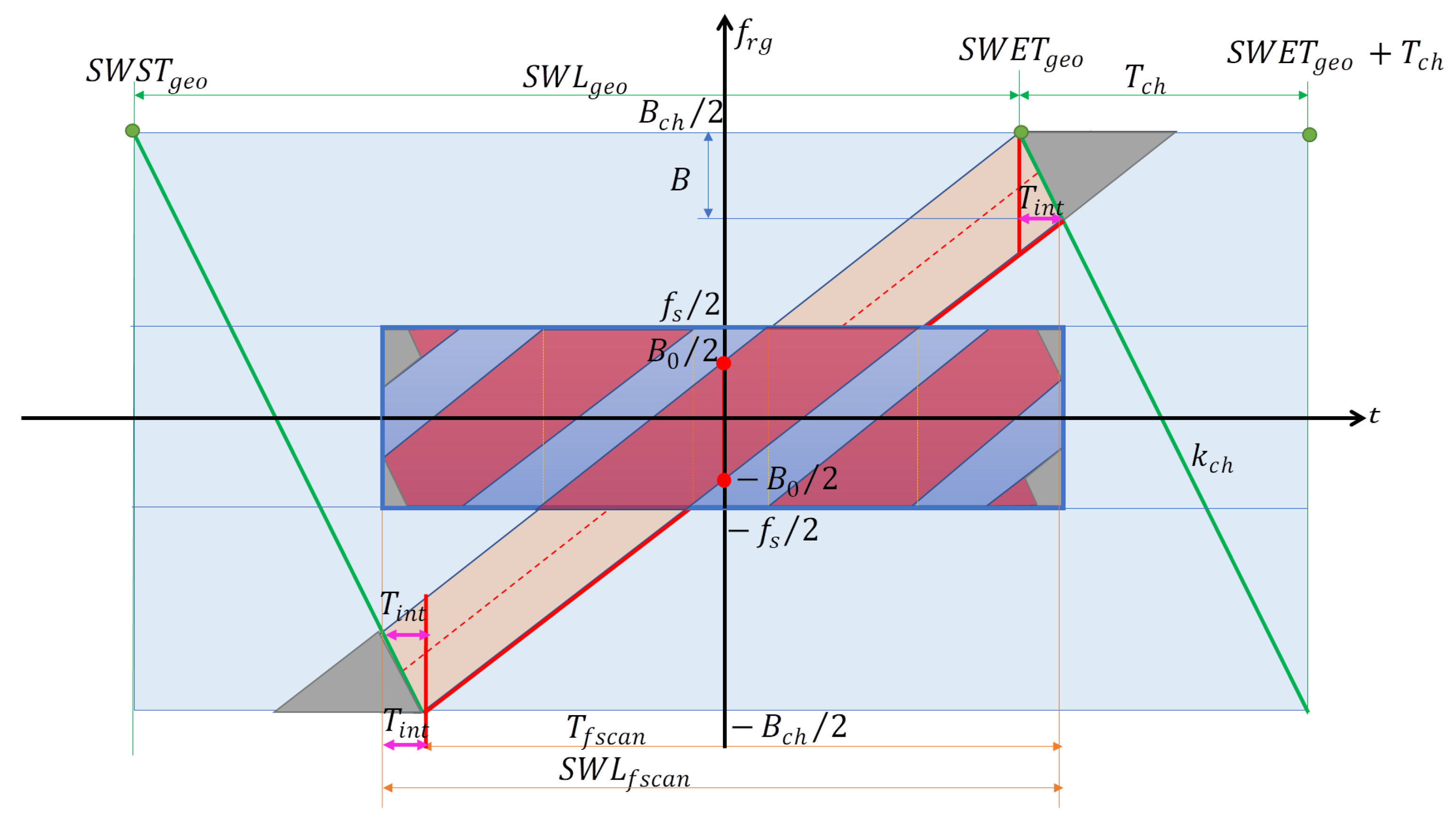
Looking at Figure 4 and Equation (13), the 2D support of the f-SCAN system is given by the product: $SW{L}_{fscan}\times f_s$, where $f_s>B_{ch}$ is the range sampling frequency. Nevertheless, it is evident that most of the domain of the data is empty, i.e., only the diagonal reddish shape contains the useful signal. Therefore, there is room for optimizing the data sampling of the received signal. We can fruitfully exploit the filtering effect of the pencil beam by allowing aliasing from those frequencies attenuated by the pencil beam itself.

Furthermore, the received SAR raw data must be sampled at a frequency: (i) significantly lower than the one required by the full band $B_{ch}$ of the transmitted chirp, but (ii) still high enough to preserve the information in the resolution band B. Indeed, the lower bound of the sampling frequency is given by the parameter $B_0$ in Figure 4, rather than by B. $B_0$ depends not only on the resolution bandwidth B, but also on both the chirp rate $k_{ch}$ and steering rate $k_{fscan}$. From the geometric considerations on Figure 4 and from Equation (14), we can write:

$$\begin{array}{cc}\hfill T_{int}=& \frac{B_0-B}{|k_{fscan}|}\hfill \\ \hfill T_{int}=& \frac{B}{|k_{ch}|}\hfill \end{array}$$

(17)

Then, by setting equal the right sides of Equation (17), we obtain the relation between $B_0$ and B:

$$B_0=\frac{|k_{fscan}|+|k_{ch}|}{|k_{ch}|}·B$$

(18)

We define as the shrinking factor of the f-SCAN acquisition the quantity:

$$k_{shrink}=\frac{|k_{ch}|}{|k_{fscan}|+|k_{ch}|}$$

(19)

Equation (19) states that the target, because of the steering rate $k_{fscan}$ of the pencil beam, experiences an antenna sharper than the physical width of the pencil beam itself. This effect is very similar to the one observed by TOPS [28] in azimuth. Moreover, Equation (19) is important because it clarifies that the minimum sampling frequency of the SAR data must be defined considering the inverse of this shrinking factor. In fact, $B_0$ is always greater than the band B necessary to fulfil the requirement of the geometric resolution. Eventually, we can take some margin $\alpha$ on $B_0$ to have the minimum sampling frequency $f_s$:

$$f_s=\alpha ·B_0<<\alpha ·B_{ch}$$

(20)

The T-F diagram of the SAR data using the reduced sampling frequency in Equation (20) is in Figure 5. The reduction of the 2D support comes from limiting both the SWL and the sampling frequency $f_s$. Compared to this, in Figure 5, there are the light blue rectangle (i.e., the extended original domain) and the blue rectangle in the centre (i.e., the new reduced domain).

The drawback of using a reduced sampling frequency is the creation of some aliasing, which would lead to “ghost” targets (which is a novel contribution to the overall ambiguity level, not to be confused with the canonical range ambiguities measured by RgDTAR). Nevertheless, the level of these ambiguous targets can be kept under control by properly choosing the sampling frequency $f_s$ and, in the case of necessity, giving a proper shape to the pencil beam, e.g., using tapering on the amplitude RX excitation coefficients. It is worth noticing that such a phenomenon is not new for SAR data as it happens along the azimuth every time the sampling frequency (i.e., PRF) is lower than the Nyquist condition. Therefore, in the instrument design stage, it would be a good choice to have a level of the range ghost comparable to (or slightly lower than) the azimuth ambiguities.

3. f-SCAN Processing

In the current section, the description of the processing of the f-SCAN data is provided. The algorithm hereinafter presented shall be applied to each received sampling window (i.e., over the fast time) at each PRI. As illustrated in Figure 5, the data are characterized by a fast time-dependent spectrum: targets at different ranges experience different central frequencies. This is the consequence of combining a wide-pulse bandwidth with a narrow pencil beam, which scans the swath using the highest directivity. Furthermore, according to the choice described in Section 2.5, the raw data spectrum is folded in frequency.

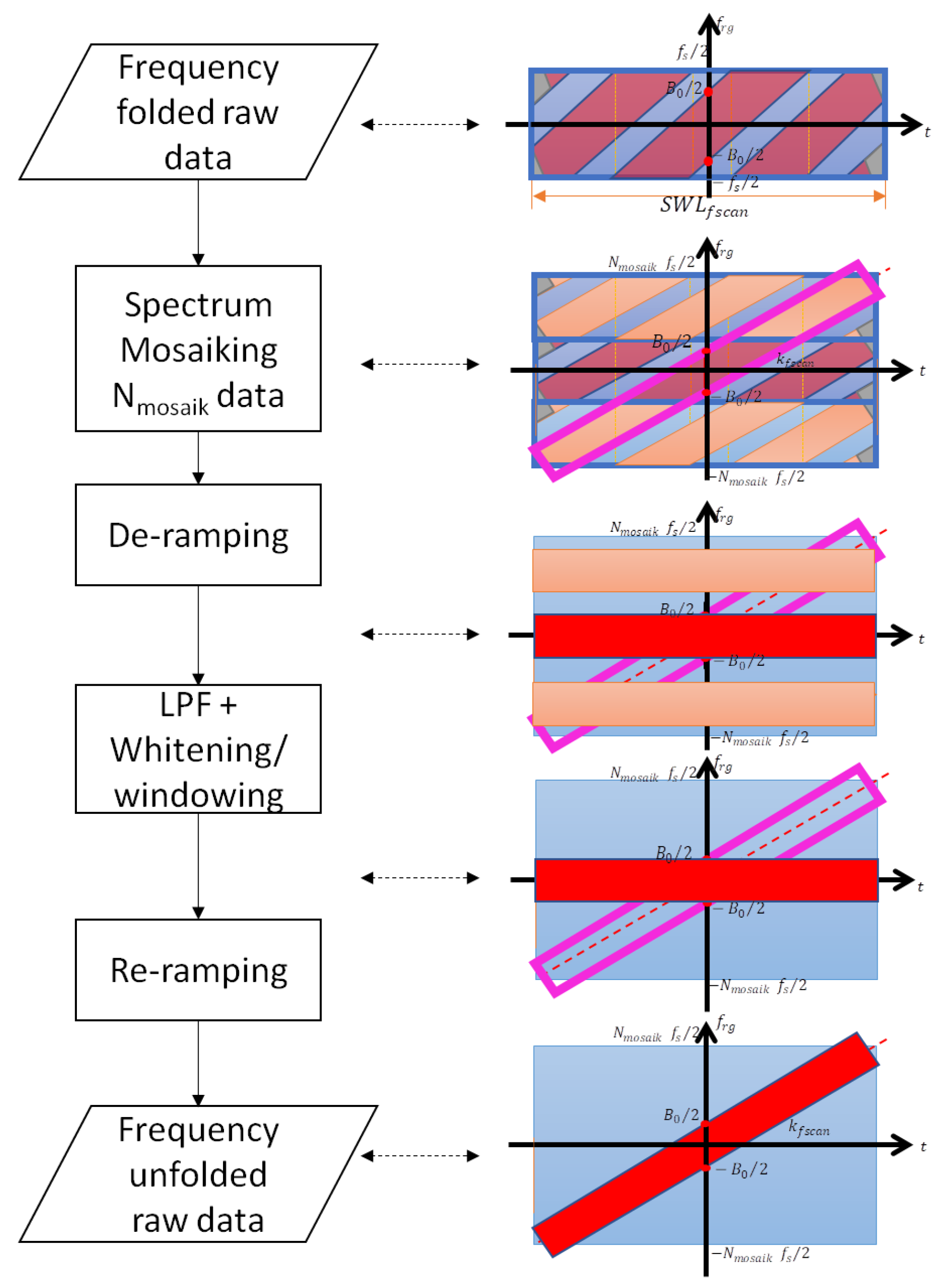
The processing of the f-SCAN data consists of: (i) restoring the full time–frequency support of the data; (ii) performing the typical SAR range compression.

The processing steps needed to restore the original frequency support of the data are shown in the block diagram of Figure 6 and hereinafter described. We remark that this algorithm shall be applied over fast time at each PRI.

First, the Fourier transform of the signal is taken and $N_{mosaik}$ copies of the spectrum are stacked. Note that the mosaicking operation is equivalent, in the time domain, to the zero interleaving of $N_{mosaik}$ samples. According to Figure 5, the number of spectral supports mosaicked is:

$$N_{mosaik}=ceil\left(\frac{B_{ch}}{B_0}\right)$$

(21)

The second step is a time-variant demodulation of the mosaicked data. This operation is known as deramping and is performed by multiplying in the time domain the SAR data times a chirp. Referring to Figure 4, the modulation rate of the deramping function is the steering rate $k_{fscan}$:

$$h_{deramp}\left(t\right)=exp\left(j\pi k_{fscan}·t^2\right)$$

(22)

with $t\in [-SW{L}_{fscan}/2,SW{L}_{fscan}/2]$. The third step is the application of a low-pass filter (LPF) to select only one spectral replica (the one in the baseband) among the $N_{mosaik}$. Please note that: (i) the nominal bandwidth of the LPF is $B_0$, according to Equation (18), and (ii) together with the LPF, it is possible to apply a whitening filter (to compensate any spectral distortion) and/or a spectral windowing to give the spectrum the desired shape. This is commonly used in SAR processing to regularize the shape of the IRF The last step to accomplish the frequency unfolding is to reramp the data by multiplying it, in the time domain, by the conjugate of Equation (22).

Once the frequency unfolding of the data is completed, the data time support is extended from $SW{L}_{fscan}$ given by Equation (13) to $SW{L}_{instr}$ given by Equation (12). This is obtained by padding the data with $N_0$ samples at the beginning and at the end, where $N_0$, according to Equation (13), is defined as:

$$N_0=\frac{B_{ch}-B}{B_{ch}/T_{ch}}·f_{s,ext}$$

(23)

Please note that, after frequency spectrum restoration, $f_{s,ext}=N_{mosaik}·f_s$ is the new sampling frequency.

At this stage, the extended support of Figure 4 has been restored from the compact support of Figure 5, and the traditional range focusing procedure can be applied, i.e., the correlation of the signal with a copy of the transmitted chirp.

Hereinafter, a mathematical description of the effects of range focusing on the data is explained. The aim was to find an equation that puts into relation the acquisition time of the raw data ($t_{acq}$) with the time of the range-focused data ($t_{foc}$). We can refer to Figure 7, where the reddish shape highlights the support of the raw data (after the unfolding procedure), whilst the yellowish shape is for the support of the range-focused data. Intuitively, the relation between the two shapes is the following: the linear dependency between time and frequency, typical of the chirp signal, is removed by the range focusing processing, and all the frequencies in the band (B) collapse in one single time instant (i.e., the time of range-focused data, $t_{foc}$). Hence, we can derive the mathematical relation between $t_{foc}$ and $t_{acq}$ by defining the quantity $f_a$ (highlighted in magenta in Figure 7) as:

$$\begin{array}{cc}\hfill f_a=& t_{acq}·\left|k_{fscan}\right|+\frac{B_0}{2}\hfill \\ \hfill f_a=& \frac{B_{ch}}{2}-\left(t_{acq}-t_{foc}\right)·\left|k_{ch}\right|\hfill \end{array}$$

(24)

Then, by making the right sides of Equation (24) equal, we obtain the relation between $t_{acq}$ and $t_{foc}$:

$$t_{acq}=\frac{\left|k_{ch}\right|}{\left|k_{ch}\right|+\left|k_{fscan}\right|}·t_{foc}+\frac{1}{2}\frac{B_{ch}-B_0}{\left|k_{ch}\right|+\left|k_{fscan}\right|}$$

(25)

where the first term takes into account the stretching of the time axis, while the second term is a constant offset.

Different from conventional SAR, for f-SCAN acquisition mode, the spectra of targets at different ranges are disjoint and not fully overlapped. This is evident from Figure 7 where the yellowish shape has a central frequency that varies with the time $t_{foc}$. The central frequency $f_{rg}$ of the target at time $t_{foc}$ is computed taking advantage of Equation (25) and $k_{fscan}$ as:

$$f_{rg}=\left|k_{fscan}\right|t_{acq}=\frac{\left|k_{ch}\right|\left|k_{fscan}\right|}{\left|k_{ch}\right|+\left|k_{fscan}\right|}·t_{foc}+\frac{B_{ch}-B_0}{2}\frac{\left|k_{fscan}\right|}{\left|k_{ch}\right|+\left|k_{fscan}\right|}$$

(26)

Thus, from the first term of Equation (26), we obtain the expression of the rate $k_{foc}$, which is the frequency modulation rate of the range-compressed data and, indeed, corresponds to the slope of the yellowish shape in Figure 7:

$$k_{foc}=\frac{\left|k_{ch}\right|\left|k_{fscan}\right|}{\left|k_{ch}\right|+\left|k_{fscan}\right|}$$

(27)

Equation (27) can be conveniently used to simplify the azimuth focusing of the f-SCAN data with respect to the processing proposed in [26]: the advantage is using a conventional (and already-existing) azimuth focusing processor. After having performed range focusing according to the algorithm previously described, the following steps are needed:

• Deramping each azimuth line from the range-compressed data according to $-k_{foc}$, where $k_{foc}$ is from Equation (27);
• Applying a standard azimuth focusing processor [29];
• Reramping each azimuth line with its natural modulation rate from Equation (27).

It is worth noting that, for the generation of standard range-compressed data and single-look complex data, it is not necessary to perform the time-variant demodulation along the range (deramping) using Equation (27) as the extended spectral support allows preserving the physical frequency at which the target has been acquired. Moreover, such residual modulation does not affect the amplitude of the single-look complex, but is still present in its phase. Therefore, all the characteristics of the target response are still preserved in the single-look complex data. On the contrary, for higher-level products (e.g., detected data), it could be useful to perform the deramping along the range, using the rate in Equation (27) to re-align the spectra of the targets along the baseband. Then, a final sub-sampling can be performed, reducing the volume of the data.

As a final remark, it is worth pointing out that, here, the most intuitive, but not optimized processing of the f-SCAN data is described. Indeed, taking advantage of the similarity between f-SCAN and the TOPS system, it is possible to define an optimized processor such as the one in [28], which directly transforms the data from the compact support of Figure 5 to those in Figure 7.

4. Exemplary System Design

In the following, the design of a realistic system is shown and the time-frequency diagrams in different stages are explained.

The system is composed of an X-band antenna acquiring a stripmap swath of about 40 km on the ground. The details of the system and geometrical parameters are given in

Table 1. System parameters.

Parameter	Value	UoM
Central frequency	9.8	GHz
Available bandwidth	1.2	GHz
Antenna height	1.5	m
No. phase centre	64
No. time delay line	8
Mechanical boresight	30	deg
PRF	2560	Hz
Duty cycle	15	%

and

Table 2. Geometric parameters.

Parameter	Value	UoM
Incidence angle interval	[21.35–25.95]	deg
Satellite height	510	km
Off-nadir angle interval	[19.70–23.90]	deg
Slant range extension	17.77	km
Ground range extension	44.28	km
Ground range resolution	1.2	m

, respectively. From the user’s point of view, the incidence angle interval and the satellite height are sufficient to define a (simplified) geometry. The remaining geometric parameters in the table (slant range, swath extension, and so on) were retrieved using geometrical relations and the local spherical Earth assumption.

By following the relations in Section 2, it is possible to obtain the timing design, as in Figure 4. Timing values are reported in

Table 3. System timing.

Parameter	Symbol	Value	UoM
Geometric SWL	$SW{L}_{geo}$	118.56	$\mathsf{\mu }$s
Instrument SWL	$SW{L}_{instr}$	177.15	$\mathsf{\mu }$s
Chirp duration	$T_{ch}$	58.59	$\mathsf{\mu }$s
Resolution time	$T_{int}$	14.84	$\mathsf{\mu }$s
Scanning time	$T_{fscan}$	74.81	$\mathsf{\mu }$s
Scanning SWL	$SW{L}_{fscan}$	89.65	$\mathsf{\mu }$s
Resolution bandwidth	B	304	MHz
Instantaneous bandwidth	$B_0$	481.80	MHz
Chirp rate	$k_{ch}$	−20.48	MHz/$\mathsf{\mu }$s
fSCAN rate	$k_{fscan}$	11.98	MHz/$\mathsf{\mu }$s
Shrink factor	$\alpha$	0.631
True time delay	$\Delta \tau$	0.410	ns
Phase shifter	${\varphi }_{ps}$	−39.34	deg

. Please note that the chirp slope $k_{ch}$ is negative. The system timing, i.e., the sequence of pulse transmission and receiving intervals, together with the true time delay and phase shifter values, is finally given in

Table 4. Pulse timing.

Parameter	Value [$\mathsf{\mu }$s]
TX pulse start (ref)	0
TX pulse end	58.59
RX pulse start	160.72
RX pulse end	191.77
Start of next pulse (PRI)	390.62

.

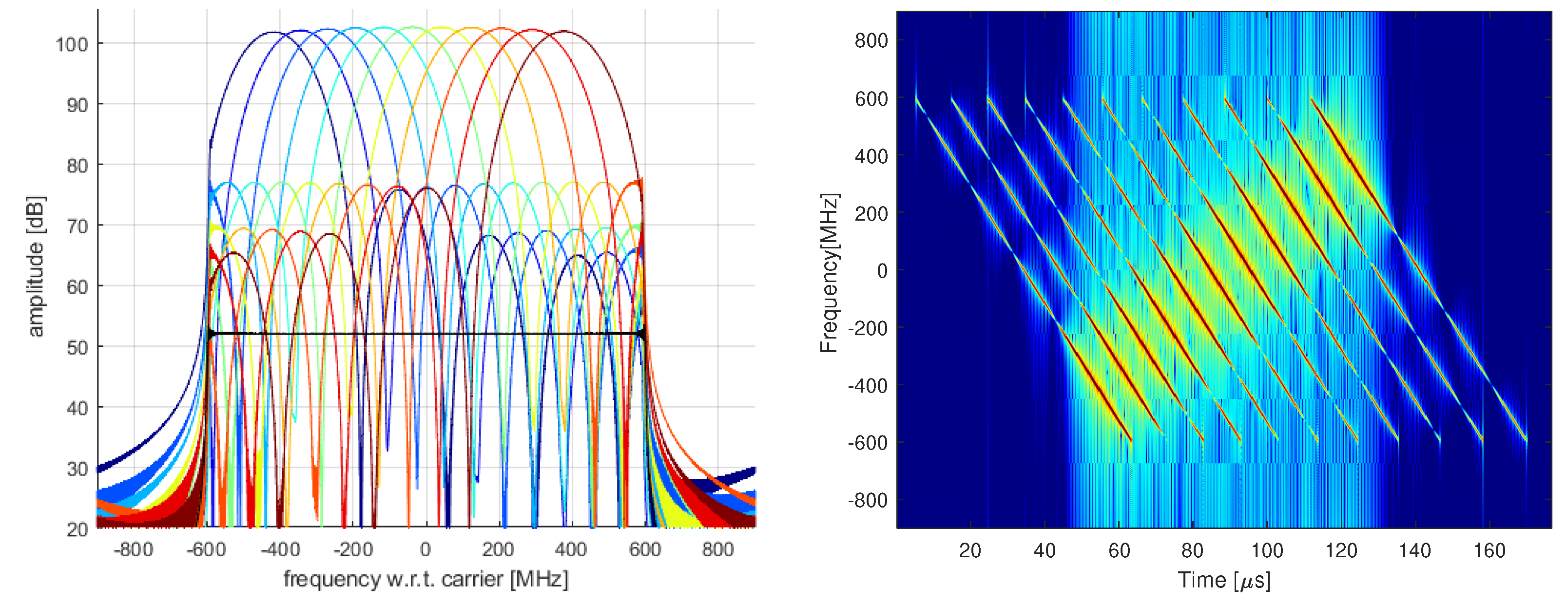
Successively, a MATLAB simulator was developed and set up with 11 ideal point targets aligned at the same azimuth and equally spaced in the off-nadir interval, from 19.9 deg to 23.68 deg (border effects were excluded). Each target was illuminated by a portion of the complete chirp due to being set in a given geometric position. Due to the antenna pattern shape (the embedded pattern of each radiator element was supposed to be a sinc shape), the frequency interval of each target was also pattern-shaped, as illustrated in Figure 8, left panel. The colour code in the figure is proportional to the frequency interval: hot colours for high frequencies; cold colours for low frequencies. Since each target generates a signal response at a different time and with different spectral support, the time–frequency diagram resulted in a sequence of lozenge supports, as shown in Figure 8, right panel.

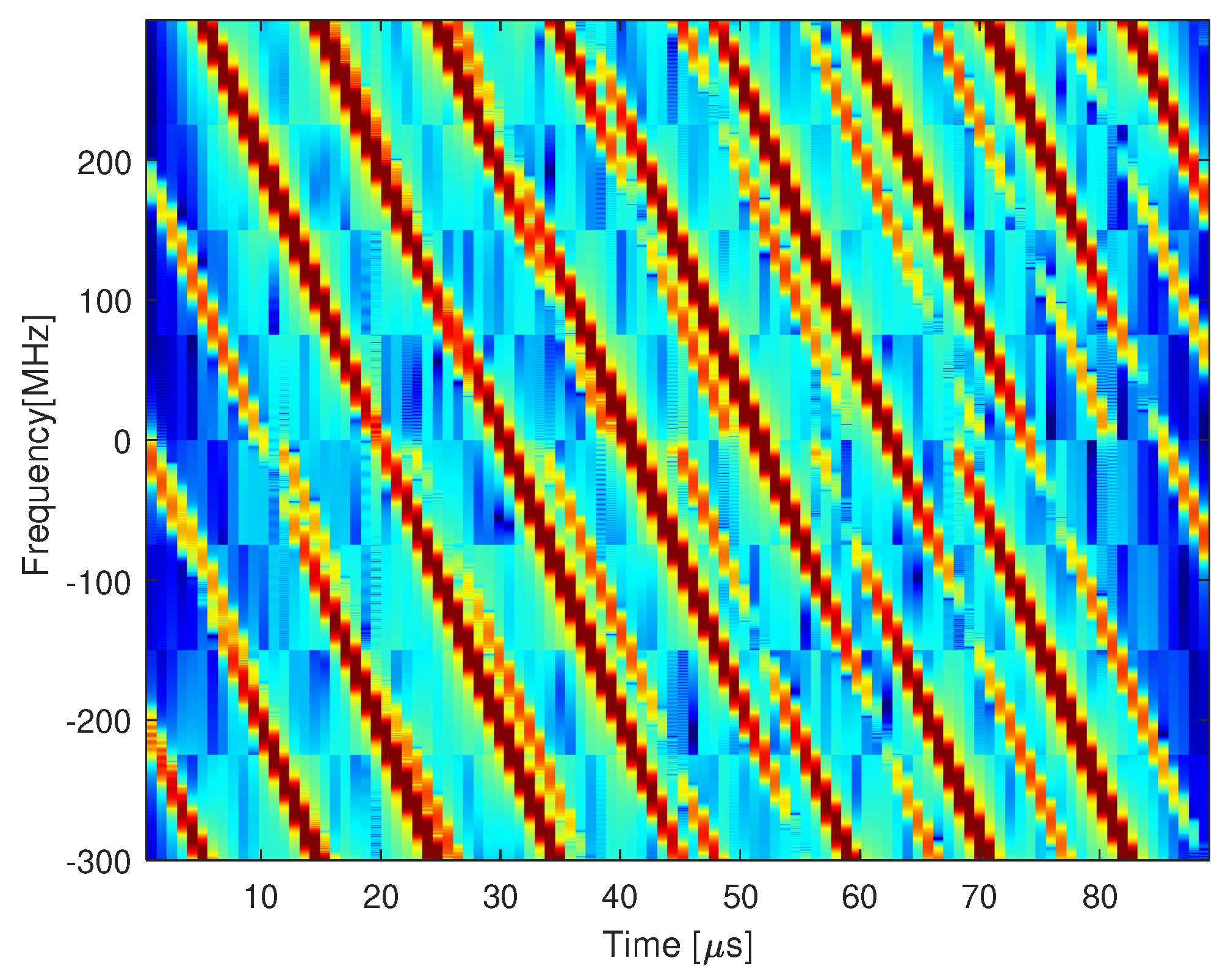
A subsampling factor equal to 3 was applied during the acquisition, so that the sampling frequency, initially set to 1.5-times the chirp bandwidth, was set to 600 MHz. Due to spectrum folding, aliasing occurs. However, the spectrograms of the different targets generate different aliasing patterns. This means that, for some of the subsampled spectrograms, the folded tails of the lozenge may overlap on the main part; in other spectrograms, they may not. This superposition, a function of the chirp and f-SCAN slopes, and the chosen sub-sampling factor make the aliasing unavoidable. This is the cost to pay to keep the range sampling frequency and the data volume low during the acquisition.

Raw data have spectral support, as reported in Figure 9. Before the range compression, they were pre-processed according to the algorithm proposed in Section 3 and illustrated in Figure 6. The steps are: (i) spectral mosaicking (by time domain zero interleaving) to raise the frequency; (ii) deramping; (iii) low-pass filtering and whitening; (iv) reramping. The (optional) whitening step was introduced to remove the antenna pattern shape of the target spectral support shown in Figure 8. Of course, whitening will raise the sidelobes, making the main lobe narrower as in traditional SAR processing, and this may be followed by a proper windowing. Conversely, whitening and windowing give the advantage of achieving an invariant IRF wherever the position of the target in the swath.

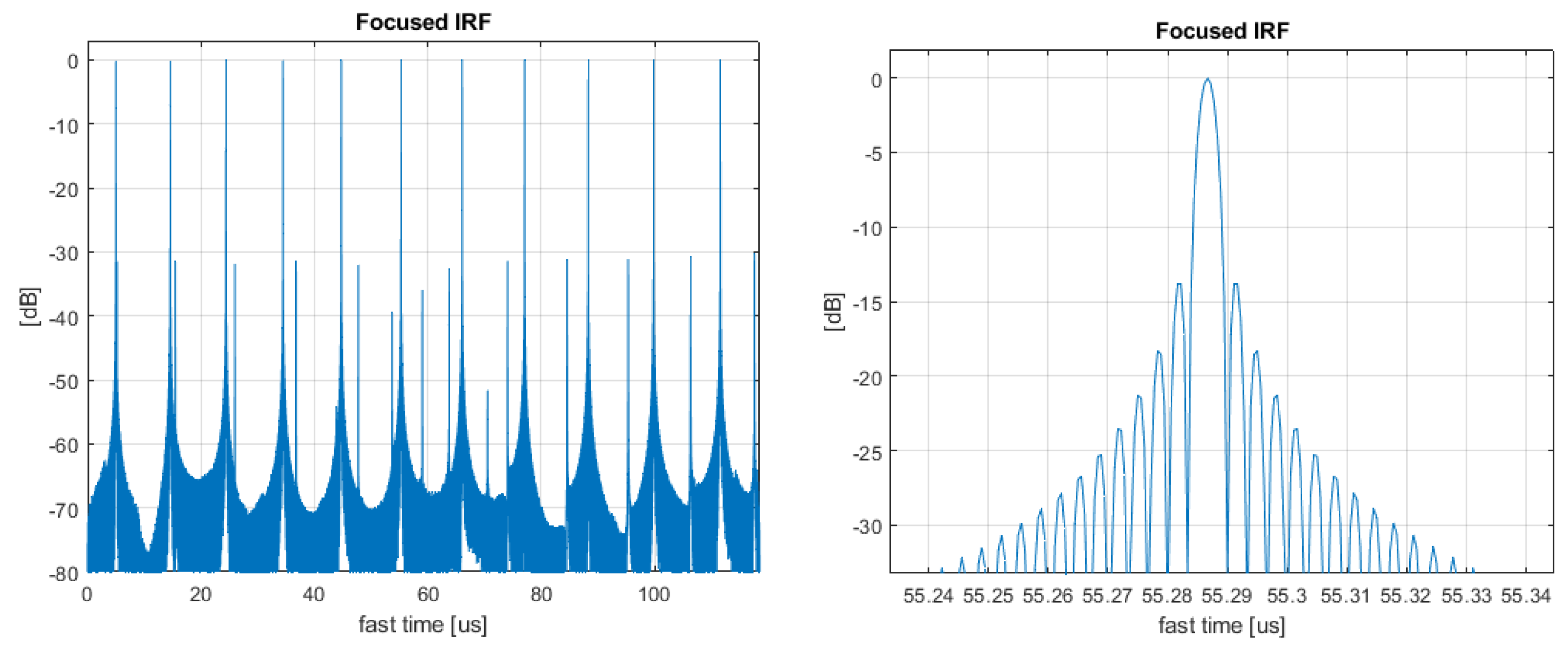
The range line after pre-processing can be compressed as in a traditional SAR system, i.e., correlating the range line with the reference pulse replica. The compressed range line is shown in Figure 10. As expected, the effect of subsampling generated spurious peaks (i.e., “ghosts”) whose level was, anyway, acceptable, being 30 dB lower than the peak. Due to the whitening (no windowing was applied in the simulation), the peak had the usual sinc shape (see Figure 10, right panel).

Quality measures of the IRF, i.e., ground range resolution, peak-to-sidelobe ratio (PSLR), and integrated sidelobe ratio (ISLR), are finally shown in Figure 11. As can be seen, the ground range resolution is within the user requirements (i.e., 1.2 m at the near range), and the PSLR and ISLR are very close to the values achieved from an ideal IRF.

5. FSCAN Performances

In this section, the typical SAR L1 performance figures are theoretically extended to the case of f-SCAN. Since f-SCAN is a method related to the elevation direction, here, we focused our attention only on the elevation-dependent parameters, i.e., the noise equivalent sigma zero (NESZ) and range-distributed target-to-ambiguity ratio (RgDTAR).

5.1. NESZ and RgDTAR Models

The traditional equation for the noise sensitivity (NESZ) [30] in the case of an f-SCAN system is modified as follows:

$$\begin{array}{cc}\hfill NES{Z}_i=& \frac{4{\left(4\pi \right)}^{3}R{\left({\theta }_i\right)}^3·kTBF·V_{s}sin\left({\theta }_i\right)·L_{SC}·L_{Az}·L}{P_{TX}·d{c}_{eff}·D_{el,2w,i}\left({\theta }_i\right)·{\lambda }_i^3·c}\hfill \\ \hfill NESZ=& {\int }_{-\Delta \theta /2}^{\Delta \theta /2}NES{Z}_i·\delta \left({\theta }_0-{\theta }_i\right)d{\theta }_i\hfill \end{array}$$

(28)

In Equation (28), $R\left({\theta }_i\right)$ is the slant range at the given off-nadir angle ${\theta }_i$; T is the temperature of noise; k is the Boltzmann’s constant; F is the noise figure of the receiver; $V_s$ is the orbital velocity of the satellite; $P_{TX}$ is the peak transmitted power; $d{c}_{eff}$ is the effective transmission duty cycle (expressed as a fraction of one), which accounts only for the part of the chirp effectively used for range compression, i.e., $d{c}_{eff}=dc·\frac{B}{B_{ch}}$; $D_{el,2w,i}\left({\theta }_i\right)$ is the two-way antenna directivity at the given angle ${\theta }_i$; ${\lambda }_i$ is the wavelength corresponding to the instrument frequency for the i-th direction; c is the light speed. The range bandwidth B is the one that drives the resolution, according to the definition in Section 2.2.

As concerns the losses, there are the traditional contributions such as the integration loss, $L_{Az}$, and all the other well-known terms summarized in L, which encompasses, e.g., TX and RX instrument losses, propagation losses, etc.

The f-SCAN system, however, experiences another kind of loss, which accounts for the effect of range spectral shaping due to the scanning pencil beam. This loss, which resembles the concept of the pulse extension loss (PEL) in SCORE [31], can be named the pulse loss, and it is addressed by $L_{SC}$ in Equation (28). It can be found by the following expression:

$$L_{SC}=\frac{{\int }_{-B/2}^{B/2}{\left|W_{rg}\left(f\right)\right|}^{2}df}{{\int }_{-B/2}^{B/2}{\left|W_{rg}\left(f\right)\right|}^2·D_{el,2w}\left(f\right)df}$$

(29)

where the term $W_{rg}\left(f\right)$ represents the contribution of the antenna whitening and windowing, if applied.

For the RgDTAR [6], the conventional formulation can be extended to f-SCAN with the same approach used for NESZ in Equation (28):

$$\begin{array}{cc}\hfill RgDTA{R}_i=& \frac{{\sum }_{n=-N}^N\frac{D_{el,2w,i}\left[\theta \left(R_i+\frac{n·c}{2·PRF}\right)\right]·{\sigma }_0\left[\theta \left(R_i+\frac{n·c}{2·PRF}\right)\right]}{sin\left[{\theta }_{inc}\left(R_i+\frac{n·c}{2·PRF}\right)\right]·{\left(R_i+\frac{n·c}{2·PRF}\right)}^3}}{\frac{D_{el,2w,i}\left[\theta \left(R_i\right)\right]·{\sigma }_0\left[\theta \left(R_i\right)\right]}{sin\left[{\theta }_{inc}\left(R_i\right)\right]·{\left(R_i\right)}^3}}\hfill \\ \hfill RgDTAR=& {\int }_{-\Delta \theta /2}^{\Delta \theta /2}RgDTA{R}_i·\delta \left({\theta }_0-{\theta }_i\right)d{\theta }_i\hfill \end{array}$$

(30)

In the previous Equation (30), ${\sigma }_0\left({\theta }_{inc}\right)$ is the reflectivity at a given incidence angle. The other terms have the same meaning as in Equation (28). In particular, the terms $R_i+n·c/2·PRF$ are the range ambiguous positions.

5.2. Comparison with No-DBF and SCORE SAR

In order to quantify the capability of the f-SCAN system, here, we compared the system defined in Section 4 with two equivalent systems: (i) a traditional SAR acquiring in stripmap mode; (ii) a SAR using digital channels in elevation to obtain SCORE. In the two cases, the chirp bandwidth was set to B = 304 MHz (to achieve the same range resolution), and the swath extension was as in the f-SCAN simulation, i.e., about 44 km. Moreover, in the case of SCORE, eight digital channels were used. In Figure 12, the comparison between the NESZ and the RgDTAR of the three systems is provided. We can clearly see that the f-SCAN outperformed the other two systems both on NESZ and the RgDTAR.

5.3. Discussion on f-SCAN’s Advantages and Drawbacks

The main advantages of f-SCAN with respect to SCORE are:

• A simpler onboard implementation. Only one receiver channel, rather than N, is required. Moreover, there is no need to have an onboard DBF recombination matrix to combine the N channels before downloading the data to the ground as the scanning of the pencil beam is achieved in the analogue domain. That means less mass (because of less hardware), volume, and power consumption.
• The chance of using the scanning high-directivity beam in both transmit and receive. Hence, the NESZ of an f-SCAN system is expected to be lower than for a SCORE system (see Figure 12).

On the other hand, f-SCAN requires:

• A more delicate design due to the close relation existing among directivity, the direction of pointing, and chirp frequency.
• A wider pulse bandwidth and, in general, a higher duty cycle, which result in higher average onboard power compared to the usual systems and to SCORE.

Finally, also f-SCAN suffers from the same impairments as SCORE, i.e., the sensitivity to timing variation due to topography. A proper redesign of the timing would be necessary in that case, as it is being analysed in the progression of DBF missions such as ROSE-L and Sentinel-1NG.

6. Conclusions

In the paper, we addressed the f-SCAN technique, which is an alternative to SCORE to achieve almost constant high directivity throughout a wide swath. f-SCAN implements the scanning beam in the analogue domain by using a proper combination of phase shifters and true time delays. The role of phase shifters and TTDLs was discussed, and a novel application was presented, aimed at extending the angle interval swept by the phase shifter only. We showed how to reduce the data volume by an effective method that involves a pre-processing step such as in TOPS SAR. The relation between the fast time of the raw data and the fast time of the range-focused data was explained, which is not trivial. Eventually, new definitions for both NESZ and RgDATR were provided. The performance of an f-SCAN system was finally compared to the corresponding performances of a SCORE system and a conventional SAR, proving the potential benefits of the former.