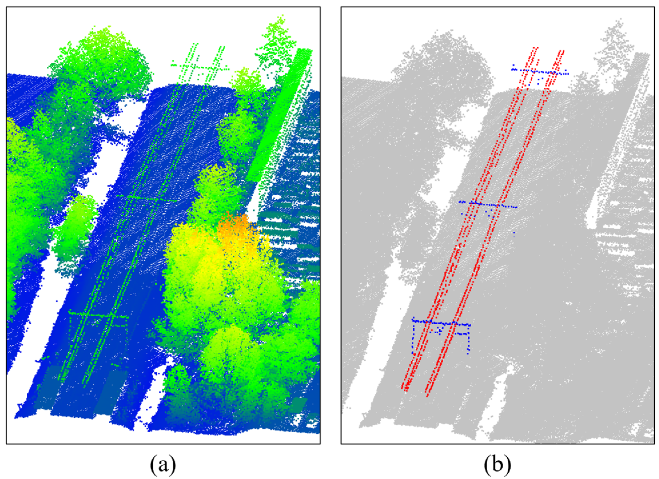
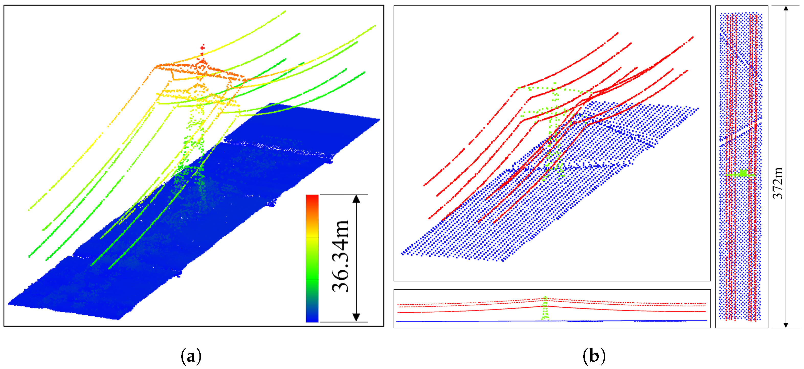
Article

A Deep Learning Based Method for Railway Overhead Wire Reconstruction from Airborne LiDAR Data

1
Key Laboratory of Quantitative Remote Sensing Information Technology, Aerospace Information Research Institute, Chinese Academy of Sciences, Beijing 100094, China
2
School of Electronic, Electrical and Communication Engineering, University of Chinese Academy of Sciences, Beijing 100049, China
3
School of Earth Sciences and Engineering, Hohai University, No.8 Fochengxi Road, Nanjing 211100, China
4
Institute of Software, Chinese Academy of Sciences, No 4, South Fourth Street, Zhong Guan Cun, Beijing 100190, China
*
Author to whom correspondence should be addressed.
Remote Sens. 2022, 14(20), 5272; https://doi.org/10.3390/rs14205272
Submission received: 14 September 2022 / Revised: 17 October 2022 / Accepted: 19 October 2022 / Published: 21 October 2022

Abstract

:
Automatically and accurately reconstructing the overhead wires of railway from airborne laser scanning (ALS) data are an efficient way of railway monitoring to ensure stable and safety transportation services. However, due to the complex structure of the overhead wires, it is challenging to extract these wires using the existing methods. This work proposes a workflow for railway overhead wire reconstruction using deep learning for wire identification collaborating with the RANdom SAmple Consensus (RANSAC) algorithm for wire reconstruction. First, data augmentation and ground points down-sampling are performed to facilitate the issues caused by insufficient and non-uniformity of LiDAR points. Then, a network incorporating with PointNet model is proposed to segment wires, pylons and ground points. The proposed network is composed of a Geometry Feature Extraction (GFE) module and a Neighborhood Information Aggregation (NIA) module. These two modules are introduced to encode and describe the local geometric features. Therefore, the capability of the model to discriminate geometric details is enhanced. Finally, a wire individualization and multi-wire fitting algorithm is proposed to reconstruct the overhead wires. A number of experiments are conducted using ALS point cloud data of railway scenarios. The results show that the accuracy and MIoU for wire identification are 96.89% and 82.56%, respectively, which demonstrates a better performance compared to the existing methods. The overall reconstruction accuracy is 96% over the study area. Furthermore, the presented strategy also demonstrated its applicability to high-voltage powerline scenarios.

1. Introduction

Railway systems have been some of the most important public transportations for decades. The overhead wires of railway, which consist of the catenary and contact wires, are the pivotal components for power supply to the system. To ensure stable and safety transportation services, regular monitoring and inspection of the wires are of crucial importance. Traditionally, in situ manual inspection or image-based automatic techniques were applied to detect irregularity and defects of the above-mentioned railway facilities [1]. However, those approaches are either labor-intensive or prone to light conditions. Light Detection and Ranging (LiDAR) integrates Laser Scanner (LS), Global Navigation Satellite System (GNSS), and Inertial Measurement Unit (IMU), which are able to sample the object of interest in the form of three-dimensional (3D) point cloud data [2]. Particularly, ALS is performed by mounting the LiDAR system on an airborne platform. By integrating the distance value to a spot illuminated by the laser pulse and the position and orientation obtained by GNSS/IMU, accurate and versatile 3D information of large scale landscape can be collected efficiently [3].
ALS has gradually become a popular method in a variety of fields due to its fast data acquisition capability [4]. Point cloud data collected by ALS have been applied in geological surveys [5,6], terrain extraction and modeling [7,8], 3D building reconstruction [9,10], forestry surveys [11,12], precision agriculture [13,14], powerline inspection [15,16], etc. Since ALS systems are able to acquire 3D shape information accurately and efficiently over a large scale, ALS point clouds have become the priority data for many related tasks such as powerline classification, extraction, and reconstruction [17,18,19]. Many existing methods can accurately extract the high-voltage powerlines [20,21,22]. However, most of these methods use classical models to extract powerlines, and there are few end-to-end methods available at present. Furthermore, railway overhead wires are more complex than high-voltage powerlines, which are mainly composed of catenary wires, support structure, and track. This structure causes the non-uniformity of the number of points in railway ALS point cloud data [23]. There are few studies on the precise extraction of railway wires from ALS data, which is still a difficult problem worthy of in-depth study.
Based on the above mentioned issues, this work proposes an automatic wires extraction algorithm for railway scenario based on ALS point cloud data. The algorithm first segments a railway corridor point cloud into three categories: wires, pylons, and ground points. Then, the extracted wire points are employed for reconstruction. The main contributions of this work are follows:
  • A data augmentation and ground point downsampling method is proposed to alleviate the non-uniformity of the number of points problem;
  • A Geometric Feature Extraction (GFE) module and a Neighbor Information Aggregation (NIA) module are introduced to combine with PointNet [24] to improve the segmentation accuracy of wires;
  • A wire individualization and multi-wire fitting method is proposed to reconstruct railway overhead wires. Figure 1 shows the applicable scenario of the proposed method.
The remaining sections are organized as follows: Related work is presented in Section 2. Section 3 and Section 4 present the details of the proposed algorithm and validation over ALS point cloud data, respectively. Conclusions are given in Section 5.

2. Related Work

Generally, powerline detection and extraction methods using point cloud data can be classified into three categories: (1) model fitting-based methods; (2) clustering-based methods; and (3) learning-based methods.

2.1. Model Fitting Based Methods

The model fitting method compares the different degrees for variance or covariance matrices between the fitting model and the observation sample, which mainly consists of Hough Transformation (HT), Least Square Method (LSM), RANSAC, etc.
A method using HT for powerline extraction from ALS point cloud data was proposed by Melzer and Briese [25]. First, terrain points were removed using digital elevation models. Then, a bottom-up HT strategy is applied iteratively to extract the powerlines. The 3D catenary lines fitting is used to reconstruct the missing powerline. Preliminary results of a 1000 m × 140 m test scan are given.
An approach using LSM for powerline extraction from ALS point cloud data was proposed by Jing et al. [26]. This method identifies points belonging to a single powerline based on the spatial distribution characteristics of the closely connected powerline points on the same powerline. Then, LSM is used to estimate the parameters of the powerline model, and multiple powerlines are reconstructed. The experimental results show that the success rate of the proposed method is 97%. However, the algorithm relies on the density of the raw data. The higher the density of the point cloud, the higher the extraction accuracy.
A method using 3D catenary models for powerline extraction from ALS point cloud data was proposed by Sohn et al. [27]. Markov Random Fields (MRF) was used for scene segmentation and accurate position of pylons with airborne urban powerline corridors. Powerlines are modeled using 3D catenary models. The extraction accuracy is 91.3%.
An algorithm that filters out the horizontal segments containing powerlines and using 2D point density-based thinning to remove trees and buildings was proposed by Yadav and Chousalkar [28]. Finally, HT is used to extract the powerlines from Mobile Laser Scanning (MLS) point cloud data. The average correctness and completeness of the urban, suburban, and rural test sites reached 98.84% and 90.84%.
A method using Principal Component Analysis (PCA) and RANSAC for powerline extraction from MLS point cloud data was proposed by Lehtomäki et al. [29]. First, MLS powerline point cloud data are voxelized in rural environments and then PCA and RANSAC are used to extract powerline and pylon points. Powerline extraction recall and precision are 93.3% and 93.6%,respectively.
The method based on model fitting has high accuracy in extracting powerlines. However, the appropriate model needs to be selected in advance, and the extraction accuracy depends heavily on data quality.

2.2. Clustering Based Methods

A clustering-based method segments a 3D point cloud dataset into different classes or clusters according to specific criteria. These criteria make use of the similarity of points in the same cluster as much as possible. The commonly used clustering approaches include K-means [30], Density-Based Spatial Clustering of Applications with Noise (DBSCAN) [31], Agglomerative NESting (AGENS) [32], etc.
A method using bottom-up point clustering for powerline extraction from MLS urban powerline point cloud data was proposed by Cheng et al. [33]. The clustering method based on the voxel is used to extract the powerline points. A bottom-up point clustering method is introduced to identify points belonging to a single powerline using 3D line fitting. The correctness and completeness of the extracted powerlines are 99.1% and 93.9%, respectively.
An approach using Euclidean distance clustering for powerline extraction from MLS powerline point cloud data was proposed by Guan et al. [34]. Road points are first separated from non-road points using threshold criteria of elevation difference and slope along the scanning trajectory. Powerlines are extracted using a combination of height filters, spatial density filters, size filters and shape filters. HT and Euclidean distance clustering were used to extract individual powerlines. The average completeness, correctness, and quality of the extracted powerlines are 92%, 99%, and 91%.
A method using a distance clustering for powerline extraction from ALS powerline point cloud data was proposed by Liang et al. [35]. Points on the same powerline will be close, while points on different powerlines will be far apart. Therefore, a method based on a distance cluster is used to extract the powerline. The experimental results show that the extraction accuracy of powerlines can reach more than 95% using this algorithm. However, this method only considers point distances, ignoring noise points that may have adverse effects.
Using a clustering-based method is able to effectively extract the powerline points. However, those methods are sensitive to the parameter settings.

2.3. Machine Learning Based Methods

Learning methods are mainly to train models to learn from data, and then use the obtained information to improve their performance. Learning methods include Decision Trees (DT), Random Forests (RF), Support Vector Machines (SVM), deep learning, etc.
Joint-Boost classification and 26 features based on geometry, intensity and multi-return information were used by Guo et al. [36] to classify the ALS powerlines. There are five categories classified: buildings, ground, vegetation, powerlines, and pylons. The average classification accuracy is 96%.
SVM is used by Wang et al. [37] to extract ALS powerline point cloud data. They use a RANSAC algorithm to construct powerline corridors and extract geometric features by calculating the oblique cylindrical neighborhood. Finally, SVM is used to obtain the results. The results show that the proposed method achieves 98%, 98%, and 97% in the extraction precision, recall, and classification quality of ALS point cloud data in urban areas.
A method using RF for powerline extraction from ALS powerline point cloud data was proposed by Peng et al. [38]. With comparing methods on powerline classification for ALS and MLS point cloud data, they found that a classification method consisting of a multi-scale vertical cylindrical neighborhood, an RF classifier, and a selected core feature set may be the best solution for balancing classification accuracy and processing time. The results show that the average precision, recall, and quality are 98%, 95%, and 93%, respectively.
Machine learning-based classification methods still have difficulty ensuring that the features used for classification contain as much information as possible. In recent years, deep learning [39] methods have shown superior performance in feature extraction [40,41], classification [42,43], and segmentation [44,45] of 3D point cloud data, which provides a new approach for powerline segmentation and extraction. A graph convolution method combining neighborhood dimensional information and neighborhood geometric information aggregation modules is proposed by Li et al. [23] to extract powerlines and pylons from ALS data. Among them, the F1 score and quality of the powerline are 99.3% and 98.6%, and the pylon scores are 96% and 92.4%. However, this method still has incomplete pylon extraction results.
High-voltage powerlines with parallel lines are extracted and reconstructed by using the above methods. However, railway wire extraction is more difficult than high-voltage lines due to the non-uniformity of the number of points caused by the railway line structure and the staggered arrangement of wires. At present, there is no automatic extraction and reconstruction method for railway overhead lines. Existing methods still need to be improved when extracting railway overhead lines. Table 1 gives the summary of the above-mentioned methods.

3. Methodology

In this section, the methodology on wire extraction and reconstruction is presented. The proposed method consists of three steps: (1) pre-processing; (2) wire segmentation; and (3) wire reconstruction. The key steps of this method are shown in Figure 2.

3.1. Pre-Processing

Due to the scanning mechanism of ALS and the characteristics of wire system, there are less numbers of points obtained on wires and pylons in comparison with that of the ground. The non-uniformity of the number of points from the above three categories will lead to oversegmentation or undersegmentation for ground and wires using a deep learning network.
To facilitate the issue, a two-step strategy is applied. First, data augmentation is conducted to ensure sufficient training data. Second, ground points are downsampled to alleviate too many numbers of points to improve model robustness.

3.1.1. Data Augmentation

Generally, with more training data, more features can be learned from the deep learning model [46]. However, there are fewer training data for existing wires. To alleviate this problem, a data augmentation strategy is introduced. This approach includes three steps: (1) Training data re-tiling, as shown in Figure 3a. The railway wire data are re-tiled along the corridor with each tile consisting of two pylons, and there is an overlap between adjacent tiles. This strategy also ensures the uniformity of the number of points to speed up network training. (2) Training data segmentation. Segment each tile into three categories: wire, pylon, and ground points (all other points). (3) Rotation amplification. Except for the original coordinates, each tile is rotated 90° about the X, Y and Z axis to obtain a new training sample, as shown in Figure 3b.

3.1.2. Ground Points Downsampling

As mentioned above, ground points usually account for more than 90% of the total points in ALS point cloud data of wire scenarios [23]. Using non-uniformity data to train the model will lead to unsatisfactory results. Therefore, the ground points are downsampled. Thus, the number of ground points and wire points is approximately equivalent. This procedure includes the following steps: (1) build an Octree of the point cloud; and (2) the center of gravity of the points in each voxel is calculated to thin the ground points. Figure 4 shows the ground point downsampling process.
Assuming P i = ( x i , y i , z i ) T is a point in a voxel, the center of gravity P g of all points in the voxel is:
P g = 1 n i = 1 n P i
Here, n is the number of points in the voxel.

3.2. Wire Segmentation

PointNet [24] is the first deep learning network to directly perform on 3D point clouds. The network only uses the x y z information of the point, which is effective on the extraction, classification and segmentation of objects of interest from point cloud data. However, it is uncertain whether the lack of the local information of the network leads to lower accuracy of the above-mentioned wire extraction.
In order to segment wires and pylons more accurately and efficiently, we propose a dual-branch network model, as shown in Figure 5. It consists of three modules: a GFE module, an NIA module and the PointNet module. The GFE module is designed to extract local geometric features of point cloud, thereby enriching local geometric information. However, local feature extraction is still challenging in extracting information in incomplete data. Thus, an NIA module is proposed to aggregate neighborhood information. The NIA module extracts the context relationship between the query point and the neighbor points, which enhances the descriptiveness of the local features of the network. The PointNet module provides point cloud alignment and rotation-invariant operations. The extracted local and global features are fed to Multi-Layer Perceptron (MLP) and max pooling to obtain the global feature of points. Finally, the features obtained by the three modules are concatenated to form 2048-dimensional features. Then, output each class scores through MLP. The proposed model is described in detail as follows.

3.2.1. GFE Module

The raw point cloud consists of only x y z coordinate values, which may be insufficient to distinguish between wires and pylons. Inspired by study [47], we find that, in wire scenes, different classes of objects vary greatly in shapes. Within a certain neighborhood, wires, pylons, and ground points are approximately linear, spherical, and have a planar structure, respectively. Therefore, three geometric feature descriptors are chosen: anisotropy, linearity, and planarity to enrich the local information of points.
Assuming a 3D point cloud set P, each point in P has x y z coordinate information. Given a query point p P and radius R, a set of neighborhood points p i | | p p i | < R is obtained. The three-dimensional structure tensor M of point cloud P in the neighborhood is defined as follows:
M = 1 n Q T Q
whereas n is number of neighborhood points. Q = ( p 1 p , p 2 p , , p n p ) T , M is a real symmetric matrix, which can be decomposed into M = R I R T , R is a rotational proof, and I is a symmetric positive definite matrix. The element of I is the eigenvalues of M. The three eigenvalues are all positive values, represented by λ 1 , λ 2 , and λ 3 , respectively, and sorted by λ 1 λ 2 λ 3 . Then, the 3D features are defined as follows:
A , L , P = ( λ 1 λ 2 ) λ 1 , ( λ 2 λ 3 ) λ 1 , ( λ 1 λ 3 ) λ 1
In case of a linear structure, such as wire points, we observe that λ 1 > > λ 2 , where a plane structure, such as ground points, λ 1 λ 2 > > λ 3 . For scattered points, such as pylon points, λ 1 λ 2 λ 3 . Through those local geometric features, we can enhance the prior knowledge of the model and improve the model’s ability to recognize objects of different shapes.
As shown in Figure 6, the radius search algorithm is used to query for n neighbor points within radius R and calculate the geometric features separately. Then, enter the PointNet model with the 3D coordinates x y z to obtain the local features of each point. Each point is represented by a six-dimensional (6D) vector, i.e., P ( x , y , z , A , L , P ) .

3.2.2. NIA Module

The GFE module enriches the input information and encompasses local shape features. However, it is difficult to completely preserve the geometric information obtained after MLP. Therefore, a short branch is introduced. It describes local details through MLP aggregate geometric shallow features. In a certain neighborhood, it is difficult for some points to have obvious geometric structures, especially at the junctions. Thus, the NIA module is proposed, which is able to extract the query point and neighboring points context information. Therefore, enhance the local geometric description capabilities of the model.
As shown in Figure 7, for a query point p q , the query point features F p q are first extracted by MLP. Then, the k original neighboring point p i | i k of the query point is found through the K Nearest Neighbors (KNN) algorithm. The neighbor features F p i after MLP are acquired through the index of point. Then, concatenate the query point features with the adjacent features to obtain the semantic features F n between points. Thus, the network can extract the local neighbor information and the context between the query point and the neighborhood points:
F n = C ( F p 0 , , F p k )
Here, C represents the concatenation of data in dimension. F n denotes the features with shape N × ( 16 × K ) .

3.2.3. Pointnet Module

The structure of PointNet module is shown in Figure 8. Each point in the input point cloud consists of a 6D feature calculated by the GEF module, i.e., P ( x , y , z , A , L , P ) . Apply the input transformation and feature transformation to the input point cloud to obtain the local features of F l each point. The point features are then aggregated through MLP and max pooling operations to obtain the global feature F g of the points:
F g = m a x ( M L P ( ( x , y , z , A , L , P ) )
Here, F g denotes the global features with shape N × 1024 and max(•) represents maxpooling operation.
As is shown in Figure 9, the MLP consists of an input layer, an output layer, and one or more hidden layers. Generally, the features are input by the input layer. The neurons in each full connection layer fit the original features and finally output the features by the output layer. High-level features obtained by MLP include multiple semantic information. However, the spatial geometric features are lacking. The low-level features obtained by the hidden layer carry more geometric details. Therefore, on the basis of aggregating local and global features, the proposed method performs multi-scale feature concatenating on the results of each layer of MLP.
The final step of the proposed method is concatenating the local and global features of the point with the neighborhood features of the NIA module to obtain the high-dimension features of each point:
F c = C ( F l , F g , F n )
Here, F c denotes the features with shape N × 2048. The proposed method uses the softmax loss function of the PointNet model:
l o s s = y i l n a i
Here, y i represents the real class, and a i represents the output value of softmax.
Finally, after MLP, the network outputs each class score. The point cloud is segmented into three types: wire, pylon, and ground point.

3.3. Wire Reconstruction

In this part, candidate wire points need to be further processed to obtain individual wire. Compared with high-voltage powerline, railway overhead wires are more complex in structure. As shown in Figure 10a, three catenary wires and one contact wire are illustrated between the two support rods. However, due to the low density of data obtained by airborne LiDAR, there are many wire disconnections. Moreover, the distance between the wires is short. Therefore, it is difficult to identify a single wire using the classical density clustering method. To facilitate the above issues, a wire identification and multi-wire fitting algorithm is designed. The algorithm is able to stably identify each wire point and reconstruct the wire by fitting the quadratic equation. The steps are presented as follows.
(1) Extraction of original wires span
The wire obtained by segmentation in the previous part is based on the data downsampled from the original data. To ensure the accuracy of wire reconstruction, reverse-mapping is performed to the original data before reconstruction. In the reverse-mapping process, the original data point is used as the query point. Kd-tree is constructed to query the nearest segmented point. The label obtained by model prediction is assigned to the query point to obtain the wire segmentation result in the original data.
The wires in railway corridors are made up of many spans, and the pylons support these spans. In the previous step, the complete pylons are extracted. The proposed method uses the coordinates of the extracted pylons to obtain their 3D bounding boxes. The wire points encompassed by the 3D bounding boxes of each span are further considered for reconstruction. Span extraction reduces the number of points and makes reconstruction of wires easier.
(2) Wire individualization
As shown in Figure 10a, the contact wire is a 3D straight line, which is on the same vertical plane as the two catenary wires above. That is, in the top view, the eight wires in the middle of the complete two support rods are arranged in parallel into four straight lines, as shown in Figure 10b. Therefore, according to this structural feature of the railway wires, an individualization and reconstruction method is proposed.
Assuming the span points set P , the proposed method obtains the eigenvector V 1 corresponding to the maximum eigenvector for the midpoint O of the bounding box, and the direction of the vector is the wire’s direction. Threshold segmentation is performed based on the distance from the point to the straight line passing through the midpoint, and the wire points are divided into four clusters: P 1 , P 2 , P 3 and P 4 . In particular, P 2 and P 3 contain three wires, two catenary wires and one contact wire, respectively. Since the two types of wires use different reconstruction models, P 2 and P 3 are divided according to the elevation to extract the contact wires.
(3) Wire reconstruction
After extracting and individualizing wires, the final step is to reconstruct the wire points for subsequent use (such as 3D measurements). It is approximated that the overhead wires in each span are nearly catenary-shaped by connecting to the consecutively pylons. As shown in Figure 10a, S 1 and S 2 are the two end points that connect the wires in red color to the pylons. Thus, all the 3D points of the wires are distributed approximately in a 2D vertical plane, which has the two end points and the corresponding wire points. The proposed method is based on the RANSAC algorithm for multi-wire fitting. The reconstruction process is described in Algorithm 1, and P is the point cluster identified in the previous step. As shown in Figure 11, the algorithm first translates P to the origin O of the global coordinate system. Then, rotate P about the Z-axis toward the X-axis by angle θ . Next, three seed points p 1 , p 2 , and p 3 are randomly selected from P to apply the quadratic model in Equation 8 for wire fitting in the XOZ plane.
z = A x 2 + B x + C
Here, A, B, C represent the parameters of the fitted catenary wires.
When the distance d from the remaining points to the fitted curve is less than the given parameter σ , the point is classified as a point on the curve. After t iterations, the model with the most wire points is taken as the optimal fit. Output the corresponding optimal parameters A b e s t , B b e s t , C b e s t . Next, loop a second curve fit on the remaining points:
z = a x + b
Here, a and b represent the parameters of the fitted contact wires.
Algorithm 1 Algorithm for multi-wire fitting.
Iuput: Point set P and initial parameter σ , t.
Output: Fitted wires parameter A, B, C and fitted points.
  1:  function ComputeFittedWireParameters
  2:     Translate P to origin O;
  3:     Rotate P about Z axis by angle θ ;
  4:     for m = 0 → 2 do
  5:        for n = 0 →t do
  6:             randomly choose seed points p 1 , p 2 , p 3 ;
  7:             determine A, B, C;
  8:             calculate the distance d from the raw wire points to z = A x 2 + B x + C ;
  9:             if d< σ  then
10:                   fitted points number++;
11:             end if
12:          end for
13:          return A b e s t , B b e s t , C b e s t corresponding to maximum fitted points number;
14:      end for
15:  end function

4. Validation

To evaluate the effectiveness of the proposed method, qualitative and quantitative evaluations are performed using ALS railway point cloud data in this section.

4.1. Data Description

As is shown in Figure 12, the proposed method is tested using the Netherlands urban railway point cloud data from the AHN3 (Het Actueel Hoogtebestand Nederland) project [48]. The details of the datasets are listed in Table 2. The whole length is approximately 7 km with 106 pylons. There are 0.18 million points with a density of 15 pts / m 2 .

4.2. Operating Environment

The environment used for the experiment of this work is a desktop with a 64-bit Linux opening system, and the deep learning framework is implemented using PyTorch. The specifications of the experimental environment are given in Table 3.

4.3. Evaluation Methods

In the wire segmentation stage, Mean Intersection over Union (MIoU) and accuracy (ACC) are used as the evaluation index. ACC represents the percentage of predicted correct results in the total sample. A lager ACC value indicates less wrong segmentation samples. However, in case of unbalanced sampling cases, ACC cannot be used as an appropriate indicator to measure the quality of segmentation results for each specific class of objects. Therefore, MIoU is employed for the overall evaluation of point cloud segmentation:
M I o U = 1 k i = 1 k T P T P + F P + F N
A C C = T P + T N T P + T N + F P + F N
where k represents k sample classes. T P (True Positive) denotes the correctly classified category. F P (False Positive) represents other parts that were incorrectly segmented into that class. F N (False Negative) means that the class is incorrectly segmented into parts of other classes. T N (True Negative) represents the other classes that are correctly classified.
In this work, there are three types of classes: wire, pylon, and groundpoint. Taking wire as an example, TP represents the wire point that is correctly predicted as wire. F P represents the point that is predicted as wire in the other two categories. F N represents the wire point that is predicted as pylon or groundpoint. In addition, T N represents the pylon and groundpoint that are correctly predicted.
In the reconstruction stage, fitting rate and fitting error are used to verify the effectiveness of the multi-wire fitting algorithm. The fitting rate indicates the proportion of the points involved in the fitting to the total number of points. The fitting error represents the average distance from the sample points to the fitting line. The lower the fitting error, the better the fitting effect:
F i t t i n g r a t e = N f i t N r a w
Here, N r a w and N f i t represent the number of points extracted by the span and the number of wire points included in the fitted curve, respectively:
F i t t i n g e r r o r = 1 n i = 1 n e d i
Here, n and e d i represent the number of fitting points and the vertical distance from the point to the fitting wire.

4.4. Parameter Settings

During preprocessing, the raw data are segmented into tiles which contain two pylons per segment. After three times of rotate amplification, a total of 392 tiles of training data were obtained. Among them, there are 280 pieces of training data, 60 pieces of test data, and the rest are validation data.
The proposed method draws on the network parameter settings of PointNet. The adaptive moment estimation was set with a momentum of 0.9. The initial learning rate is 0.001 and decreases by half every 20 epochs. The batch size is 40, and the number of training epochs is 200.
In the railway wires scenario, the non-uniformity of the number of the points dramatically reduces the final segmentation accuracy. Therefore, we focus on the effect of the choice of radius R on the extraction of pylon points when calculating geometric features. The effect of anisotropy on point cloud segmentation by changing the R value is shown in Figure 13. Specifically, we set R = 2 m, R = 4 m, or R = 6 m. The figure shows the anisotropy value of each point in a tile of point cloud data calculated under different radius and its distribution range. When R = 2 m, there is no obvious effect on the extraction of the pylon; when R = 4 m, the value of the pylon points is more obvious compared to other points; when R = 6 m, the anisotropy value of ground points around the pylon and a part of the wire points are close to the pylon points, which can easily produce error classification. Thus, the geometric feature extraction radius of the railway overhead wires is set to 4 m.
According to the selection of the above R, we found that the number of neighborhood points at the center point below the R radius is within 2 to 4. Therefore, in the NIA module, the k of the 3-Nearest Neighbor algorithm is set to 3.
In the wire reconstruction, we choose σ = 0.1, 0.15, 0.2 and t = 50 to fit the railway overhead wires. As shown in Figure 14, as the σ increases, the average fitting error from the original single wire to the fitted wire increases gradually. At the same time, however, the number of fitting points tends to remain unchanged. After comprehensive consideration, σ = 0.15 and t = 50 are finally selected to fit the wires. All parameters are given in Table 4.

4.5. Pre-Processing Results

After pre-processing, a sample tile of training data is shown in Figure 15. Table 5 gives the comparison of various target points of the tiles of training data after ground points downsampling.

4.6. Wire Segmentation

4.6.1. Training Results

As shown in Figure 16, the preprocessed data are trained by the proposed model. As the training is carried out, the loss of the training set continues to decline. When the number of iterations reaches 100, the loss trends to convergence. The accuracy in the training set also stabilized at 100 iterations. It can be seen from the trend of the loss of test set that the initial loss is around 1.0. With the progress of training, the loss gradually decreased and tended to converge after 100 rounds. There is no significant difference between training loss and test loss, which indicates that the model training effect is more effective. The accuracy of the test set is also rising with the convergence of the model. According to the trend of the training set loss and the accuracy of the test set, it can be seen that the proposed model is able to effectively segment the wire.

4.6.2. Model Verification

To further verify the effectiveness and robustness of the proposed method, the proposed method is compared with existing segmentation methods, which use PCA to calculate geometric features. After filtering nearby places, the wire and pylon are classified by setting reasonable thresholds. The experiment results are also compared with the PointNet method.
Table 6 and Figure 17 show the quantitative and qualitative comparison of different methods, respectively. The classification accuracy of PCA method of the railway overhead wires reaches 84.38%, and MIoU reaches 0.6029. As seen from area A and B in Figure 17a denoted by the rectangles, using the classical segmentation method PCA to segment the wire will produce a large error, especially at pylon and wire connections. Compared with the traditional method, the MIoU and ACC of wire segmentation are improved by 22.36% and 12.51% when using the proposed method. The reason is that the proposed method extracts more features than the PCA method.
Compared with PointNet, the proposed method also has great advantages. Particularly, PointNet barely learns the correct features when segmenting wires, resulting in severe segmentation errors, in area C, D, and E in Figure 17b denoted by the rectangles. On the contrary, the proposed method improves MIoU and ACC by 38.05% and 22.95%, respectively. Figure 17c also shows that the objects extracted by the proposed method are intact. There are only sporadic points misclassifications, as shown in rectangle F. This is due to the neighborhood points and local geometric information involved in the proposed method, which enables learning more detailed features.

4.6.3. Effectiveness of Each Proposed Module

In order to evaluate the effectiveness of the proposed module, a series of ablation experiments are designed. Table 7 shows the performance changes of the model after adding different modules. As shown in Table 7, PointNet has a lower precision segmentation effect in the railway scene.
The GFE module is designed to enrich the input information and provide local geometric features for the network. Table 7 shows that, after introducing the GFE module, the railway overhead wires, MIoU and ACC, increased by 35.52% and 22.19%, respectively. This shows that the local geometric features obtained by GFE module can greatly enrich input features, thereby improving the segmentation accuracy.
As discussed in Section 3, the local geometry provided by the GFE module cannot be completely retained after MLP. Therefore, the NIA module aims to aggregate neighborhood information to enhance the ability to describe local features. Table 7 gives comparative results. It can be seen that, after employing the NIA module, the proposed method has further improved compared to “PointNet+GFE”. Compared with PointNet, MIoU and ACC increased by 36.63% and 22.59% in railway extraction. This proves the validity of adding aggregate neighbor information to the network.
We propose to gather low-level information extracted from the hidden layer in PointNet MLP to high-level information, thereby enhancing the details of the points. Compared with PointNet, in the railway extract, MIoU and ACC increased by 38.05% and 22.95%, respectively.

4.7. Wire Reconstruction

The wire individualization and reconstruction results are shown in Figure 18 and Figure 19. Figure 18 is the original wire mapping and span extraction process; Figure 19a,b is the wire individualization based on the XOY plane; Figure 19e is the fitting result of the wire. The curve is basically consistent with the original point distribution. As shown in Table 8 and Figure 20, the average fitting rate of the wire over the three spans is 96.29%. The average fitting error is 0.053 m. The experimental results show that the method can efficiently realize the reconstruction of railway overhead wires. As shown in Figure 19e, the omitted part of the wire is also well rebuilt.

4.8. Applicability of High-Voltage Powerline Scenarios

4.8.1. High-Voltage Line Data and Pre-Processing Results

The proposed method is also applicable for powerline extraction in high-voltage line scenarios. The method is validated using the ALS high-voltage line point cloud data shown in Figure 21a. Figure 21b is the tile of training data after pre-processing. Different from the railway data, the distance between the two pylons of the high-voltage line is relatively large. Moreover, there are relatively many points of one pylon. Therefore, the principle of each tile of data including one pylon is used for segmentation, and the ground point downsampling is used to alleviate the effect of the non-uniformity of the points.

4.8.2. Model Verification

The quantitative and qualitative results of the model’s powerline extraction in high-voltage powerline scenarios are shown in Table 9 and Figure 22, with the extraction accuracy and MIoU reaching 98.52% and 89.94%, respectively. Figure 22a shows that only sporadically two pylon points are mis-segmented as powerline points.

5. Discussion and Conclusions

Experiments show that the proposed method is able to effectively extract, identify, and reconstruct railway overhead wires. Moreover, the proposed method only uses ALS point cloud data containing xyz coordinate information, making the proposed method more widely applicable. The superior results of our method can be attributed to the following reasons:
  • In the preprocessing step, the proposed data augmentation method effectively solved the non-uniformity of the number of the points of the ALS railway point cloud data.
  • In the wire segmentation step, the proposed GFE and NIA modules effectively obtain geometric features and semantic information.
  • In the wire reconstruction step, the proposed wire individualization and multi-wire fitting method robustly fits the severe omitted railway overhead wires.
This work proposes a new method based on PointNet network for efficient and accurate extraction of railway overhead wires from ALS point cloud data. First, in the railway scene, an effective data augmentation and ground points downsampling method is proposed for the problem of the non-uniformity of the number of the points. Secondly, based on the PointNet network, a dual branch network method is introduced. The upper branch uses the local geometric information obtained by the GFE module to extract local and global features through a PointNet network. The lower branch uses the NIA module to enhance local neighborhood information. Then, the new point feature is extracted by MLP based on the point feature combined by the upper and lower branches. Finally, a wire individualization and multi-wire fitting algorithm is proposed to reconstruct railway overhead wires. Experiments show that the proposed method can effectively extract railway overhead wires. The ACC and MIoU of the overhead wires’ segmentation reached 96.98% and 82.65%, respectively. The fitting rate and fitting error of the multi-wire fitting method is above 96% and 0.05 m. Last but not the least, the proposed method is also applicable to automatic high-voltage powerline scenario segmentation.

Author Contributions

Conceptualization, L.Z. and J.W.; methodology, L.Z. and J.W.; software, L.Z. and J.W.; validation, Y.C. and Y.S.; formal analysis, Y.S. and J.L.; investigation, L.C. and M.Z.; data curation, Y.C. and L.Z.; writing-original draft preparetion, L.Z. and J.W.; writing-review and editing, L.Z. and J.W.; visualization, L.Z. and J.W.; supervision, J.W.; project administration, M.Z.; funding acquisition, J.W. and M.Z. All authors have read and agreed to the publish version of the manuscript.

Funding

This research was funded by the National Natural Science Foundation of China (NSFC) under the grants No 61771456 and 42201487 and was also funded by project of Chinese Academy of Sciences granted with No E1330603.

Data Availability Statement

The data and code are open via this webpage: https://github.com/zhanglele98/Wire-Reconstruction (accessed on 13 September 2022).

Conflicts of Interest

The authors declare no conflict of interest.

References

  1. Wei, H.; Zhu, H.; Wang, Z.; Wu, W. Center Line Coordinates Survey for Existing Railway by 3D Constraints Method. TELKOMNIKA Indones. J. Electr. Eng. 2013, 11, 2816–2821. [Google Scholar] [CrossRef]
  2. Luo, S. The Airborne Laser Radar Technology and Its Application in Power Engineering. Shanxi Sci. Technol. 2015, 30, 115–156. [Google Scholar]
  3. Vosselman, G.; Hans-Gerd, M. Airborne and Terrestrial Laser Scanning; Whittles Publishing: Dunbeath, UK, 2011; pp. 19–30. [Google Scholar]
  4. Li, X.; Guo, Y. Application of LiDAR technology in power line inspection. IOP Conf. Ser. Mater. Sci. Eng. 2018, 382, 052025. [Google Scholar] [CrossRef]
  5. Hosford, S.; Baghdadi, N.; Bourgine, B.; Daniels, P.; King, C. Fusion of airborne laser altimeter and RADARSAT data for DEM generation. In Proceedings of the International Geoscience and Remote Sensing Symposium (IGARSS), Toulouse, France, 21–25 July 2003. [Google Scholar] [CrossRef]
  6. Chiu, C.L.; Fei, L.Y.; Liu, J.K.; Wu, M.C. National airborne LiDAR mapping and examples for applications in deep-seated landslides in Taiwan. In Proceedings of the International Geoscience and Remote Sensing Symposium (IGARSS), Milan, Italy, 26–31 July 2015. [Google Scholar] [CrossRef]
  7. Sithole, G.; Vosselman, G. Experimental comparison of filter algorithms for bare-Earth extraction from airborne laser scanning point clouds. ISPRS J. Photogramm. Remote Sens. 2004, 59, 85–101. [Google Scholar] [CrossRef]
  8. Rasib, A.W.; Ismail, Z.; Rahman, M.Z.; Jamaluddin, S.; Kadir, W.H.; Ariffin, A.; Razak, K.A.; Kang, C.S. Extraction of Digital Terrain Model (DTM) over vegetated area in tropical rainforest using LiDAR. In Proceedings of the International Geoscience and Remote Sensing Symposium (IGARSS), Melbourne, VIC, Australia, 21–26 July 2013. [Google Scholar] [CrossRef]
  9. Wang, Q.; Ni-Meister, W.; Ni, W.; Pang, Y. The Potential of Forest Biomass Inversion Based on Canopy-Independent Structure Metrics Tested by Airborne LiDAR Data. In Proceedings of the International Geoscience and Remote Sensing Symposium (IGARSS), Yokohama, Japan, 28 July–2 August 2019. [Google Scholar] [CrossRef]
  10. Huang, H.; Brenner, C.; Sester, M. A generative statistical approach to automatic 3D building roof reconstruction from laser scanning data. Isprs J. Photogramm. Remote. Sens. 2013, 79, 29–43. [Google Scholar] [CrossRef]
  11. Aicardi, I.; Dabove, P.; Lingua, A.M.; Piras, M. Integration between TLS and UAV photogrammetry techniques for forestry applications. IForest 2017, 10, 41–47. [Google Scholar] [CrossRef] [Green Version]
  12. Wang, Y.; Sun, Y.; Liu, Z.; Sarma, S.E.; Bronstein, M.M.; Solomon, J.M. Dynamic graph Cnn for learning on point clouds. ACM Trans. Graph. 2019, 38, 1–12. [Google Scholar] [CrossRef]
  13. Garrido, M.; Paraforos, D.S.; Reiser, D.; Arellano, M.V.; Griepentrog, H.W.; Valero, C. 3D maize plant reconstruction based on georeferenced overlapping lidar point clouds. Remote Sens. 2015, 7, 17077–17096. [Google Scholar] [CrossRef] [Green Version]
  14. Li, W.; Niu, Z.; Wang, C.; Huang, W.; Chen, H.; Gao, S.; Li, D.; Muhammad, S. Combined Use of Airborne LiDAR and Satellite GF-1 Data to Estimate Leaf Area Index, Height, and Aboveground Biomass of Maize during Peak Growing Season. IEEE J. Sel. Top. Appl. Earth Obs. Remote Sens. 2015, 8, 4489–4501. [Google Scholar] [CrossRef]
  15. Ituen, I.; Sohn, G. The way forward: Advances in maintaining right-of-way of transmission lines. Geomatica 2010, 64, 451–462. [Google Scholar]
  16. Pu, S.; Xie, L.; Ji, M.; Zhao, Y.; Liu, W.; Wang, L.; Zhao, Y.; Yang, F.; Qiu, D. Real-time powerline corridor inspection by edge computing of uav lidar data. Int. Arch. Photogramm. Remote Sens. Spatial Inf. Sci. 2019, XLII-2/W13, 547–551. [Google Scholar] [CrossRef] [Green Version]
  17. Matikainen, L.; Lehtomäki, M.; Ahokas, E.; Hyyppä, J.; Karjalainen, M.; Jaakkola, A.; Kukko, A.; Heinonen, T. Remote sensing methods for power line corridor surveys. ISPRS J. Photogramm. Remote Sens. 2016, 119, 10–31. [Google Scholar] [CrossRef] [Green Version]
  18. Xu, S.; Wang, R. Power Line Extraction From Mobile LiDAR Point Clouds. IEEE J. Sel. Top. Appl. Earth Obs. Remote Sens. 2019, 12, 734–743. [Google Scholar] [CrossRef]
  19. Nardinocchi, C.; Balsi, M.; Esposito, S. Fully Automatic Point Cloud Analysis for Powerline Corridor Mapping. IEEE Trans. Geosci. Remote Sens. 2020, 58, 8637–8648. [Google Scholar] [CrossRef]
  20. Ceron, A.; Mondragon B., I.F.; Prieto, F. Power line detection using a circle based search with UAV images. In Proceedings of the 2014 International Conference on Unmanned Aircraft Systems, ICUAS 2014—Conference Proceedings, Orlando, FL, USA, 27–30 May 2014. [Google Scholar] [CrossRef]
  21. Munir, N.; Awrangjeb, M.; Stantic, B. An improved method for pylon extraction and vegetation encroachment analysis in high voltage transmission lines using LiDAR data. In Proceedings of the 2020 Digital Image Computing: Techniques and Applications, DICTA 2020, Melbourne, Australia, 29 November–2 December 2020. [Google Scholar] [CrossRef]
  22. Huang, Y.; Du, Y.; Shi, W. Fast and accurate power line corridor survey using spatial line clustering of point cloud. Remote Sens. 2021, 13, 1571. [Google Scholar] [CrossRef]
  23. Li, W.; Luo, Z.; Xiao, Z.; Chen, Y.; Wang, C.; Li, J. A GCN-Based Method for Extracting Power Lines and Pylons from Airborne LiDAR Data. IEEE Trans. Geosci. Remote Sens. 2022, 60, 1–14. [Google Scholar] [CrossRef]
  24. Qi, C.R.; Su, H.; Mo, K.; Guibas, L.J. PointNet: Deep learning on point sets for 3D classification and segmentation. In Proceedings of the 30th IEEE Conference on Computer Vision and Pattern Recognition, CVPR 2017, Honolulu, HI, USA, 21–26 July 2016; pp. 77–85. [Google Scholar] [CrossRef] [Green Version]
  25. Melzer, T.; Briese, C. Extraction and Modeling of Power Lines from ALS Point Clouds. In Proceedings of the 28th Workshop of the Austrian Association for Pattern Recognition, Hagenberg, Austria, 22–23 May 2004. [Google Scholar]
  26. Jing, L.; Zhang, J.; Deng, K.; Liu, Z.; Shi, Q. A New Power-Line Extraction Method Based on Airborne LiDAR Point Cloud Data. In Proceedings of the 2011 International Symposium on Image and Data Fusion, Tengchong, China, 9–11 August 2011. [Google Scholar]
  27. Sohn, G.; Jwa, Y.; Kim, H.B. Automatic powerline scene classification and reconstruction using airborne LiDAR data. In Proceedings of the ISPRS Annals of the Photogrammetry, Remote Sensing and Spatial Information Sciences, Melbourne, Australia, 25 August–1 September 2012. [Google Scholar] [CrossRef] [Green Version]
  28. Yadav, M.; Chousalkar, C.G. Extraction of power lines using mobile LiDAR data of roadway environment. Remote Sens. Appl. Soc. Environ. 2017, 8, 258–265. [Google Scholar] [CrossRef]
  29. Lehtomäki, M.; Kukko, A.; Matikainen, L.; Hyyppä, J.; Kaartinen, H.; Jaakkola, A. Power line mapping technique using all-terrain mobile laser scanning. Autom. Constr. 2019, 105, 102802. [Google Scholar] [CrossRef]
  30. MacQueen, J. Some Methods for Classification and Analysis of Multivariate Observations. In Proceedings of the 5th Berkeley Symposium on Mathematical Statistics and Probability—Vol. 1; Le Cam, L.M., Neyman, J., Eds.; University of California Press: Berkeley, CA, USA, 1967; pp. 281–297. [Google Scholar]
  31. Ester, M.; Kriegel, H.P.; Sander, J.; Xu, X. A Density-Based Algorithm for Discovering Clusters in Large Spatial Databases with Noise. In Proceedings of the 2nd International Conference on Knowledge Discovery and Data Mining, Portland, OR, USA, 2–4 August 1996. [Google Scholar]
  32. Agglomerative Hierarchical Clustering. In Clustering Methodology for Symbolic Data; John Wiley & Sons, Ltd.: Hoboken, NJ, USA, 2019; Chapter 8; pp. 261–316. [CrossRef]
  33. Cheng, L.; Tong, L.; Wang, Y.; Li, M. Extraction of Urban Power Lines from Vehicle-Borne LiDAR Data. Remote Sens. 2014, 6, 3302–3320. [Google Scholar] [CrossRef] [Green Version]
  34. Guan, H.; Yu, Y.; Li, J.; Ji, Z.; Zhang, Q. Extraction of power-transmission lines from vehicle-borne lidar data. Int. J. Remote Sens. 2016, 37, 229–247. [Google Scholar] [CrossRef]
  35. Liang, J.; Zhang, J.; Liu, Z. On extracting power-line from airborne LiDAR point cloud data. Bull. Surv. Mapp. 2012, 7, 17–20. [Google Scholar]
  36. Guo, B.; Huang, X.; Zhang, F.; Sohn, G. Classification of airborne laser scanning data using JointBoost. ISPRS J. Photogramm. Remote Sens. 2015, 100, 71–83. [Google Scholar] [CrossRef]
  37. Wang, Y.; Chen, Q.; Liu, L.; Zheng, D.; Li, C.; Li, K. Supervised classification of power lines from airborne LiDAR data in Urban Areas. Remote Sens. 2017, 9, 771. [Google Scholar] [CrossRef] [Green Version]
  38. Peng, S.; Xi, X.; Wang, C.; Dong, P.; Wang, P.; Nie, S. Systematic comparison of power corridor classification methods from ALS point clouds. Remote Sens. 2019, 11, 1961. [Google Scholar] [CrossRef]
  39. Lecun, Y.; Bengio, Y.; Hinton, G. Deep Learning. Nature 2015, 521, 436–444. [Google Scholar] [CrossRef]
  40. Lu, X.; Zhong, Y.; Zheng, Z.; Liu, Y.; Zhao, J.; Ma, A.; Yang, J. Multi-Scale and Multi-Task Deep Learning Framework for Automatic Road Extraction. IEEE Trans. Geosci. Remote Sens. 2019, 57, 9362–9377. [Google Scholar] [CrossRef]
  41. Chen, J.; Lei, B.; Song, Q.; Ying, H.; Chen, D.Z.; Wu, J. A Hierarchical Graph Network for 3D Object Detection on Point Clouds. In Proceedings of the IEEE Computer Society Conference on Computer Vision and Pattern Recognition, Seattle, WA, USA, 14–19 June 2020. [Google Scholar] [CrossRef]
  42. Geng, J.; Wang, H.; Fan, J.; Ma, X. SAR image classification via deep recurrent encoding neural networks. IEEE Trans. Geosci. Remote Sens. 2018, 56, 2255–2269. [Google Scholar] [CrossRef]
  43. Xu, M.; Ding, R.; Zhao, H.; Qi, X. PAConv: Position Adaptive Convolution with Dynamic Kernel Assembling on Point Clouds. In Proceedings of the IEEE Computer Society Conference on Computer Vision and Pattern Recognition, Nashville, TN, USA, 20–25 June 2021. [Google Scholar] [CrossRef]
  44. Mou, L.; Zhu, X.X. Vehicle Instance Segmentation from Aerial Image and Video Using a Multitask Learning Residual Fully Convolutional Network. IEEE Trans. Geosci. Remote Sens. 2018, 56, 6699–6711. [Google Scholar] [CrossRef] [Green Version]
  45. Hu, Q.; Yang, B.; Xie, L.; Rosa, S.; Guo, Y.; Wang, Z.; Trigoni, N.; Markham, A. Randla-Net: Efficient semantic segmentation of large-scale point clouds. In Proceedings of the IEEE Computer Society Conference on Computer Vision and Pattern Recognition, Seattle, WA, USA, 14–19 June 2020. [Google Scholar] [CrossRef]
  46. Hamraz, H.; Jacobs, N.B.; Contreras, M.A.; Clark, C.H. Deep learning for conifer/deciduous classification of airborne LiDAR 3D point clouds representing individual trees. ISPRS J. Photogramm. Remote Sens. 2019, 158, 219–230. [Google Scholar] [CrossRef] [Green Version]
  47. Lalonde, J.F.; Vandapel, N.; Huber, D.F.; Hebert, M. Natural terrain classification using three-dimensional ladar data for ground robot mobility. J. Field Robot. 2006, 23, 839–861. [Google Scholar] [CrossRef]
  48. AHN3 Download. Available online: https://app.pdok.nl/ahn3-downloadpage/ (accessed on 25 August 2022).
Figure 1. An applicable scenario of the proposed methodology. (a) point cloud data of a railway scenario (The points are colorized by height from red to blue); (b) overhead wires are automatically segmented and reconstructed by the proposed method.
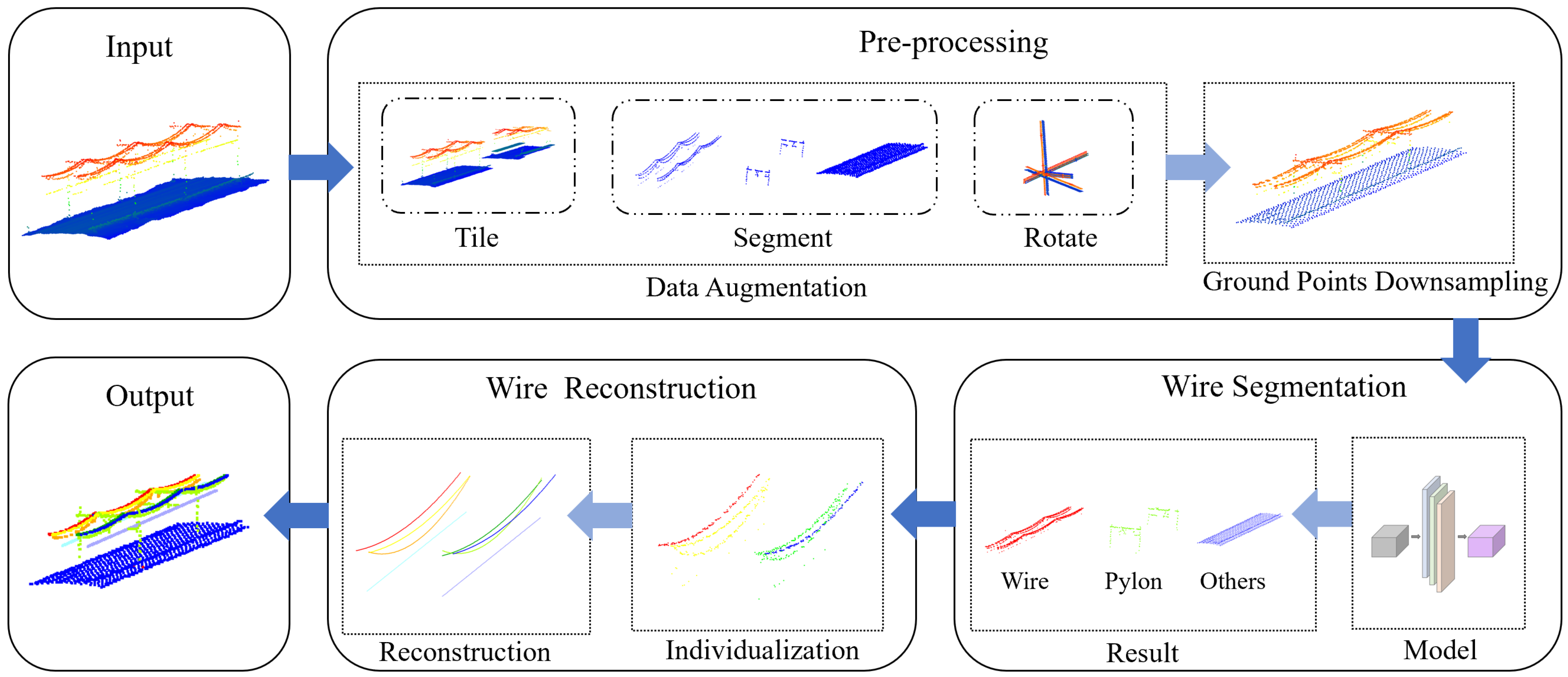
Remotesensing 14 05272 g001
Figure 2. The overall procedure of the proposed method. First, raw data are preprocessed to obtain training data. Then, training data are fed into the proposed model for wire segmentation. Consecutively, the segmentation results are used for wire reconstruction.
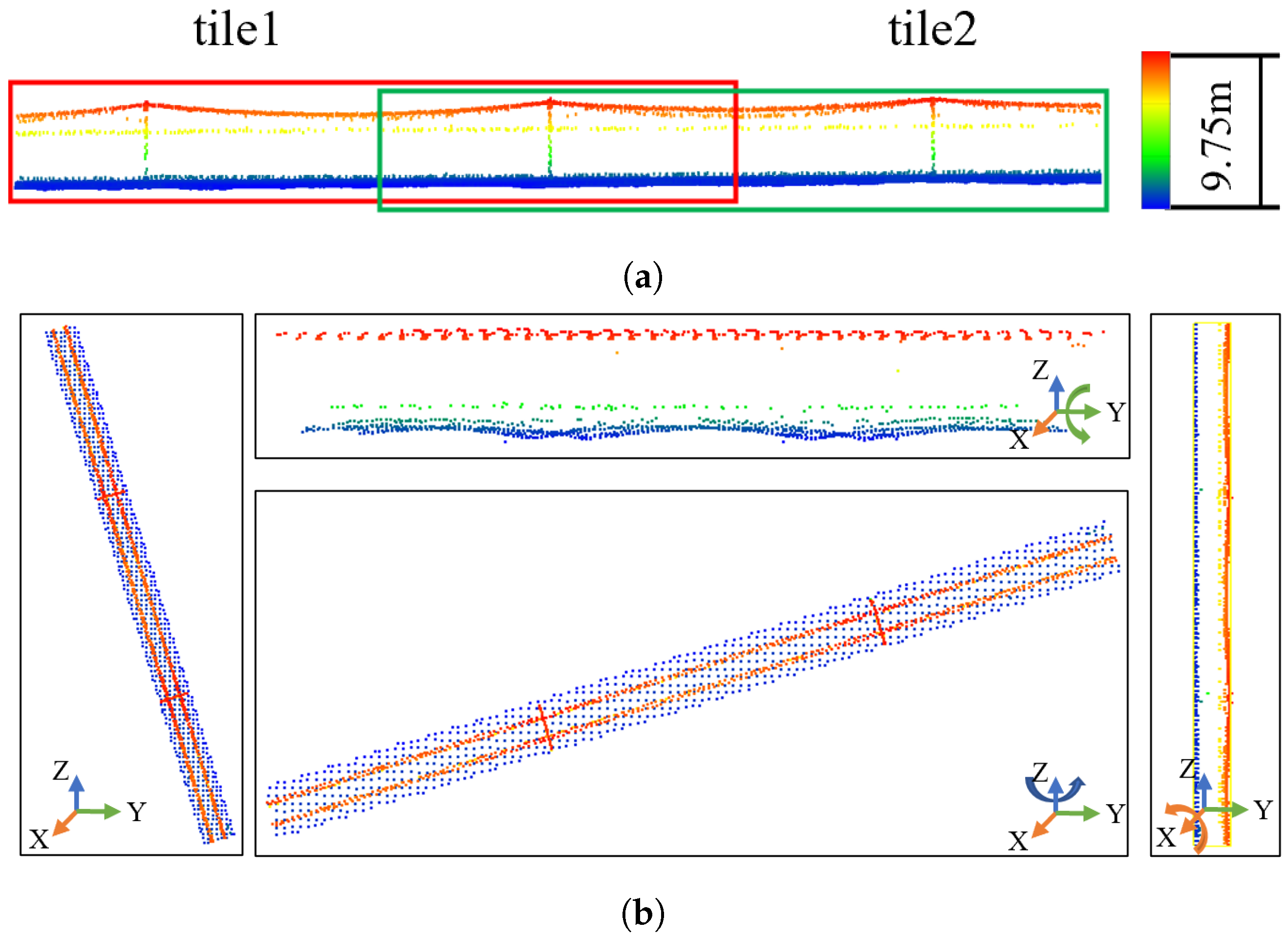
Remotesensing 14 05272 g002
Figure 3. Data augmentation. (a) training data re-tiling; (b) rotation amplification. The four images are the visualization of the original tile and the rotated tile on the XOY plane.
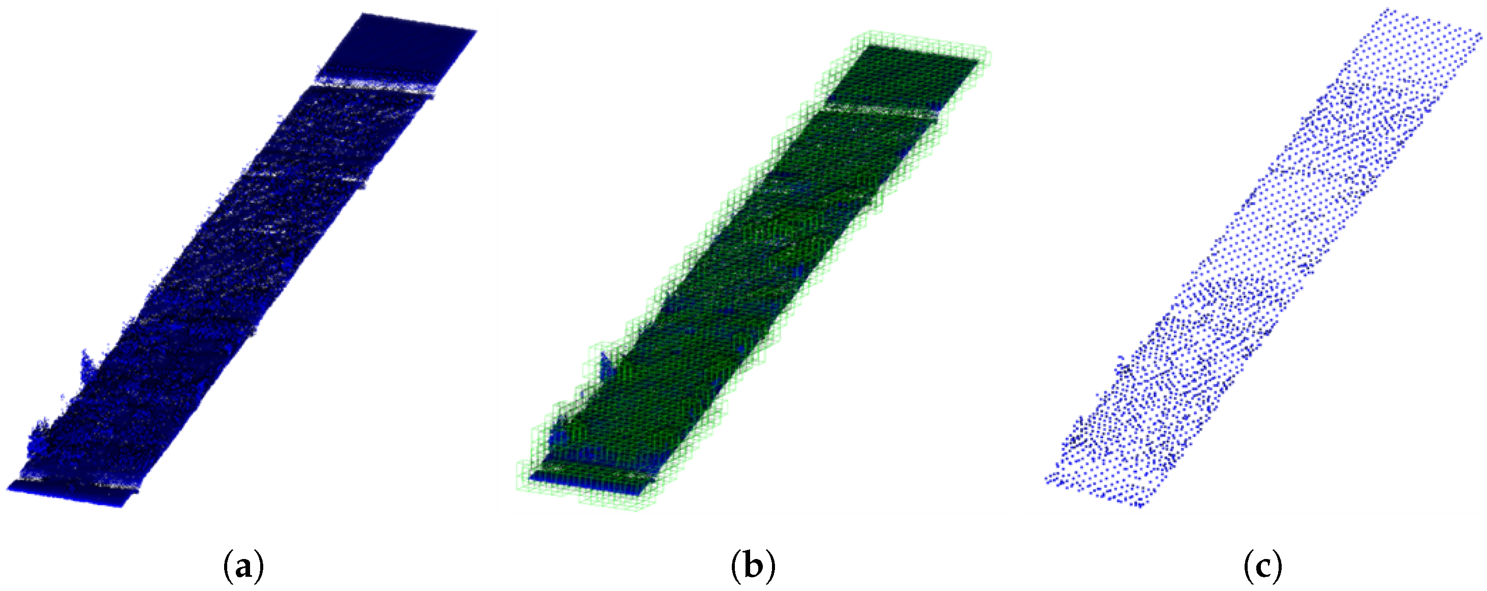
Remotesensing 14 05272 g003
Figure 4. Ground point downsampling. (a) original ground point cloud; (b) an Octree space division of the ground points; (c) downsampling the ground points.
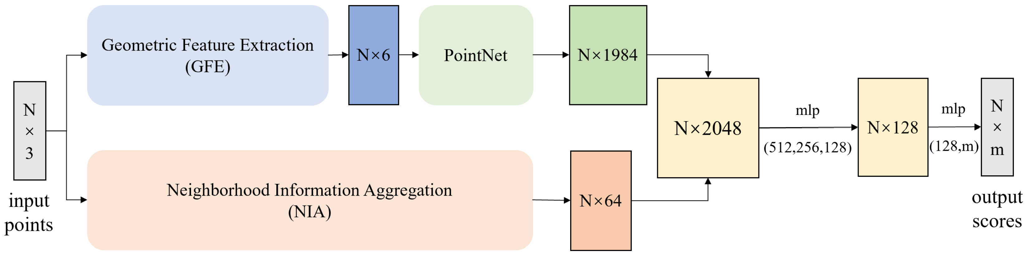
Remotesensing 14 05272 g004
Figure 5. Flowchart of the presented model in this work. The GFE module extracts local geometric features of point cloud. The NIA module aggregates neighborhood feature information. The PointNet module outputs each class score through MLP.
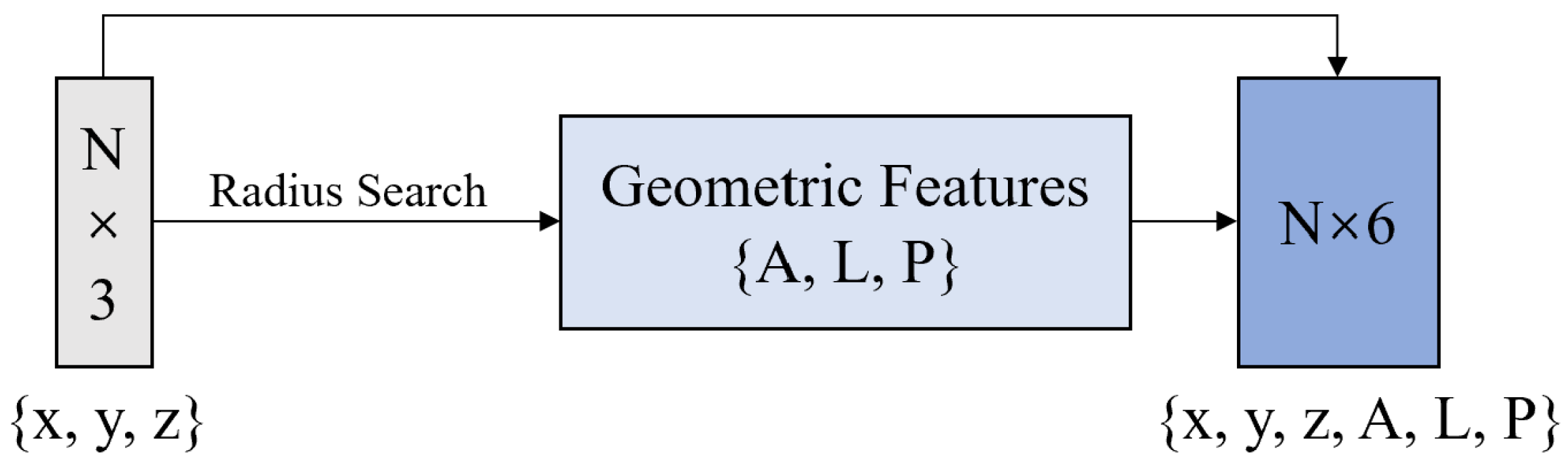
Remotesensing 14 05272 g005
Figure 6. Network structure of the GFE module.
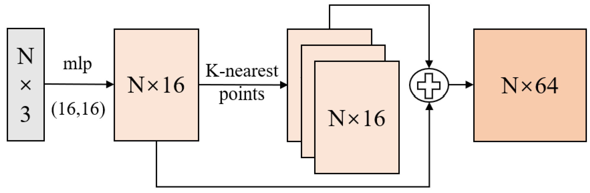
Remotesensing 14 05272 g006
Figure 7. Network structure of the NIA module.
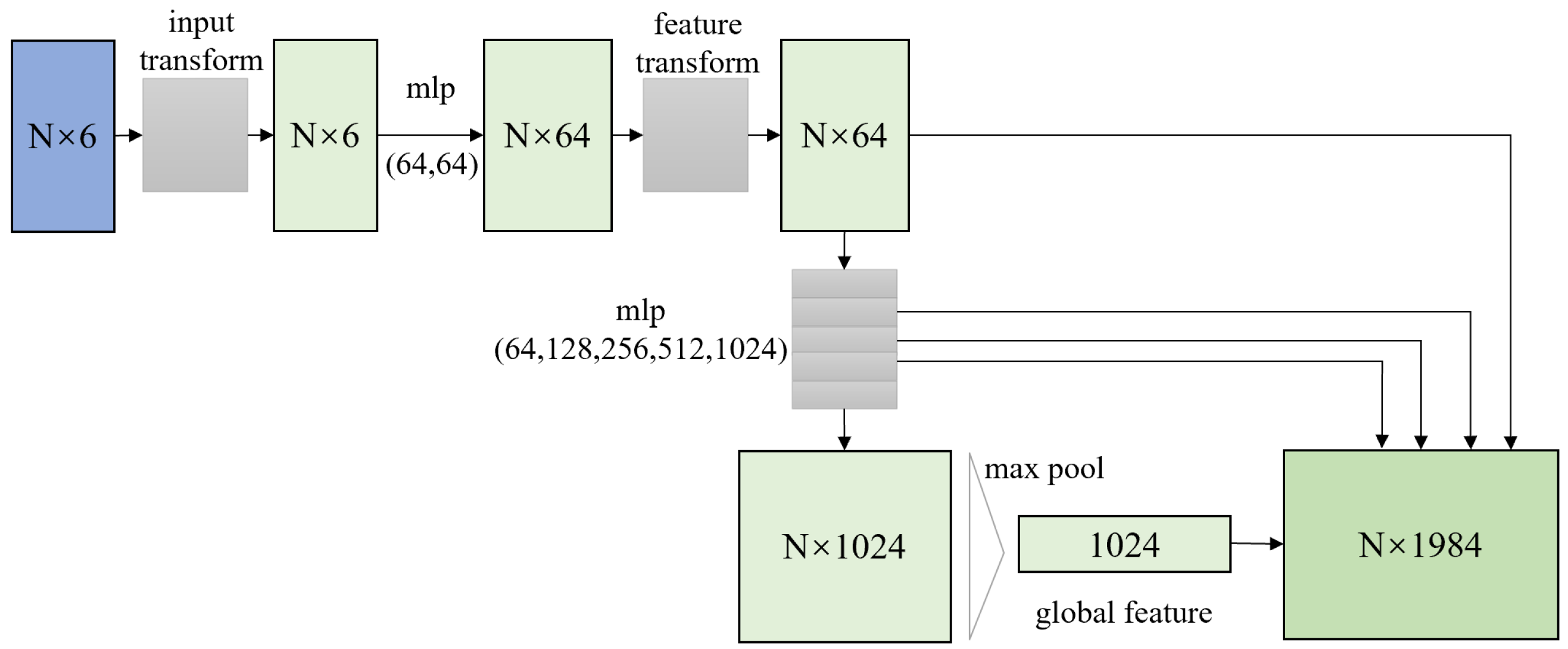
Remotesensing 14 05272 g007
Figure 8. Network structure of the PointNet module.
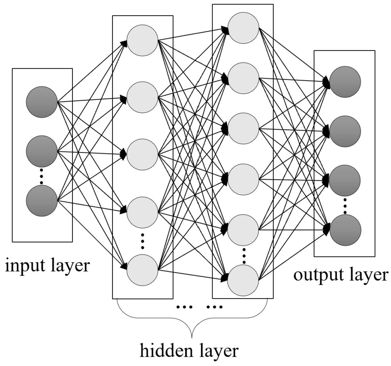
Remotesensing 14 05272 g008
Figure 9. Multi-layer perception (MLP) structure.
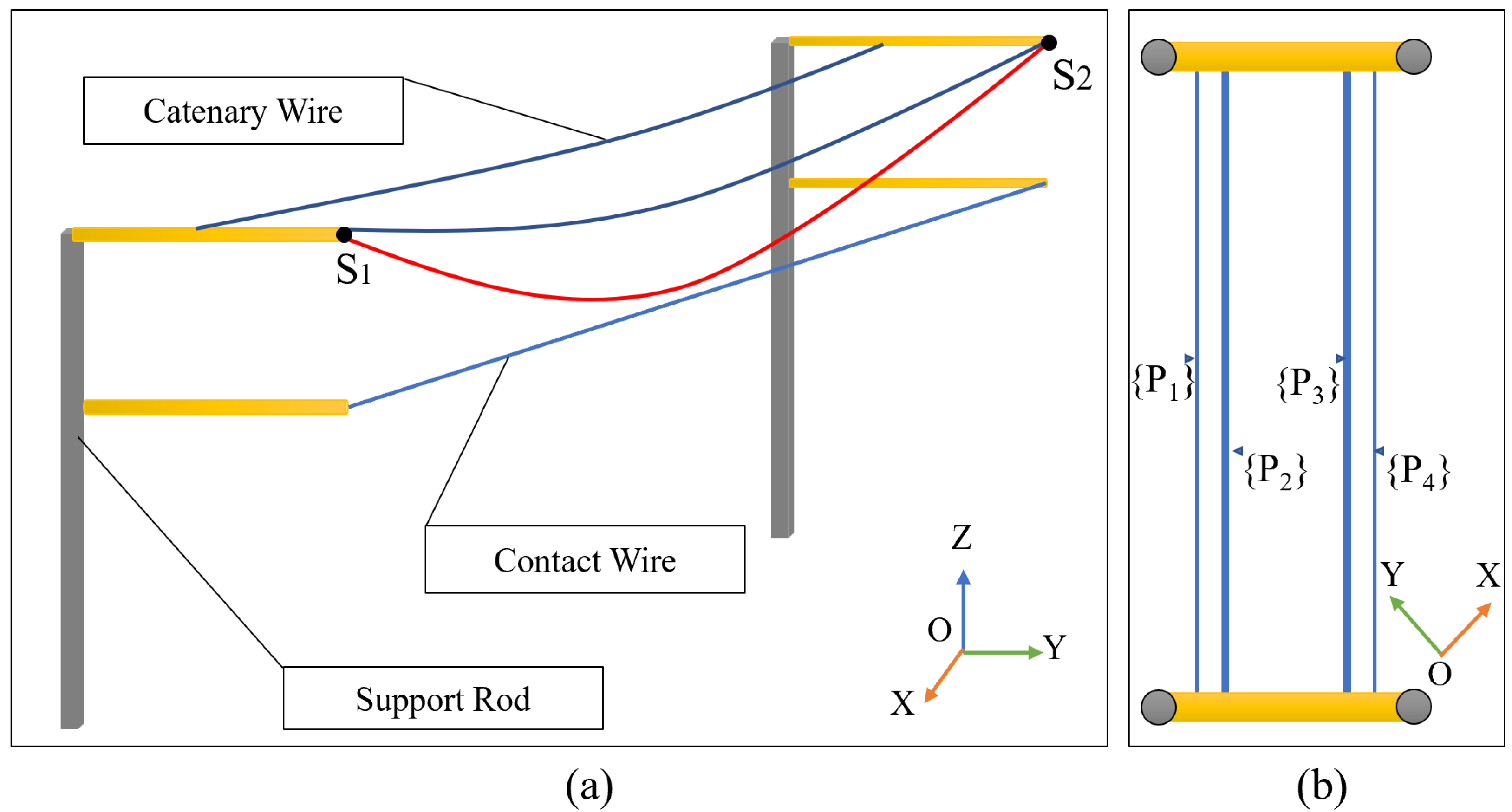
Remotesensing 14 05272 g009
Figure 10. Schematic diagram of the structure of the railway overhead wires (a) side view; (b) top view.
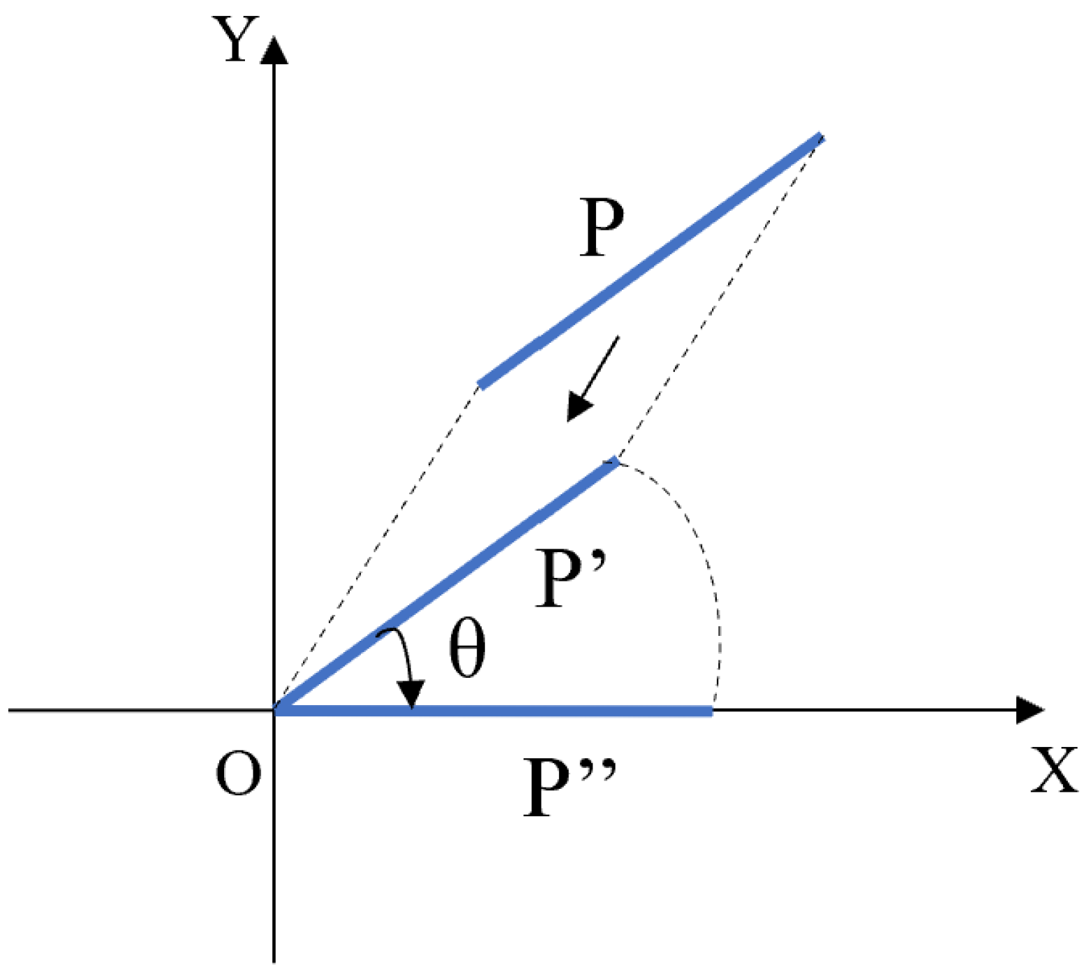
Remotesensing 14 05272 g010
Figure 11. Transformation procedures of the point set P in the XOY plane.
Remotesensing 14 05272 g011
Figure 12. The railway dataset used by the proposed method.
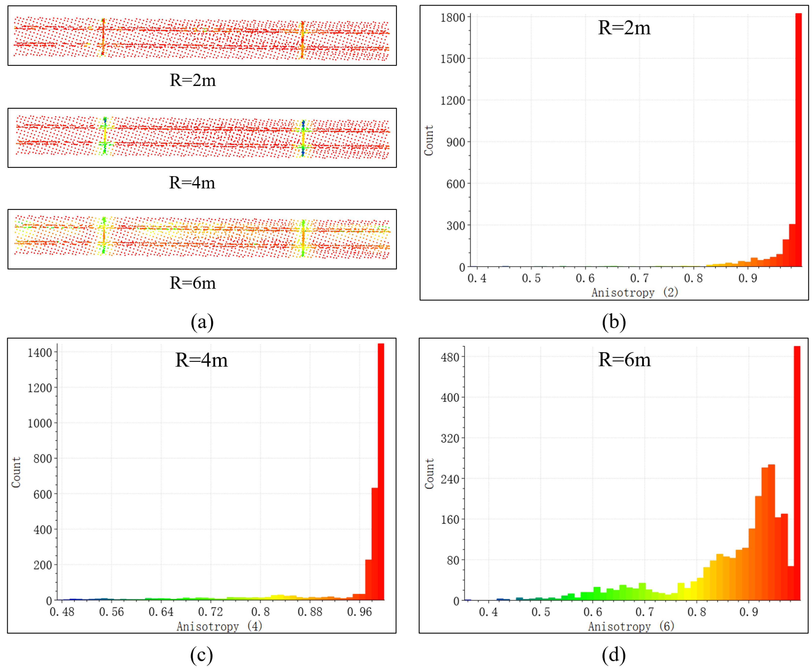
Remotesensing 14 05272 g012
Figure 13. The anisotropy value with different neighbourhood radius. (a) anisotropy values with radius 2, 4, and 6 m; (bd) are the distributions of anisotropy value with the radius, respectively.
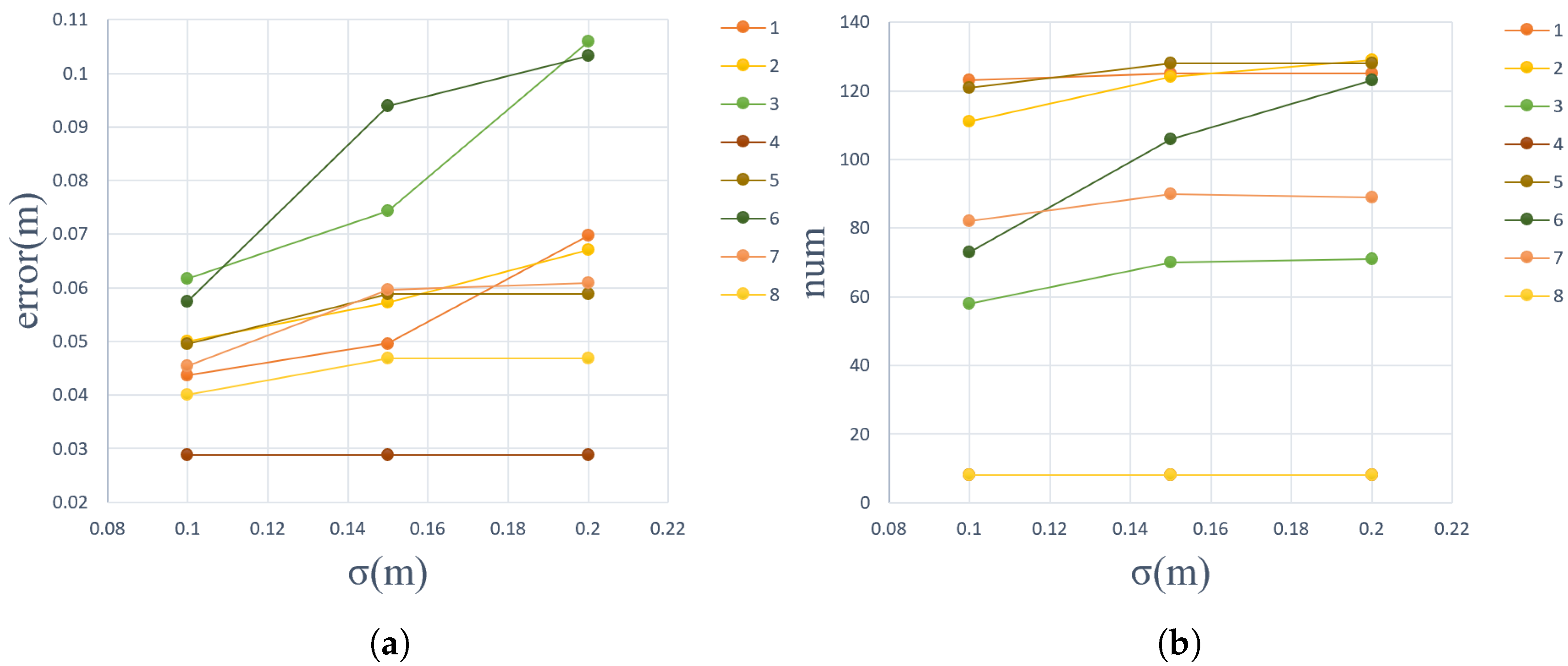
Remotesensing 14 05272 g013
Figure 14. The influence of the choice of σ on the fitting effect. (a) the average fitting error of a single wire under different σ ; (b) the number of points fitted by a single wire under different σ (1–8 represent 8 wires in a span respectively).
Remotesensing 14 05272 g014
Figure 15. Training data from different perspectives after preprocessing (red, green and blue points represent wire, pylon, and ground points, respectively).
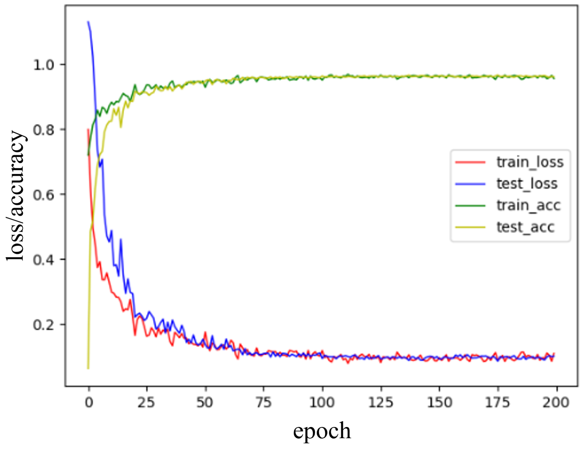
Remotesensing 14 05272 g015
Figure 16. The trend of the training and test sets loss/accuracy during the model training.
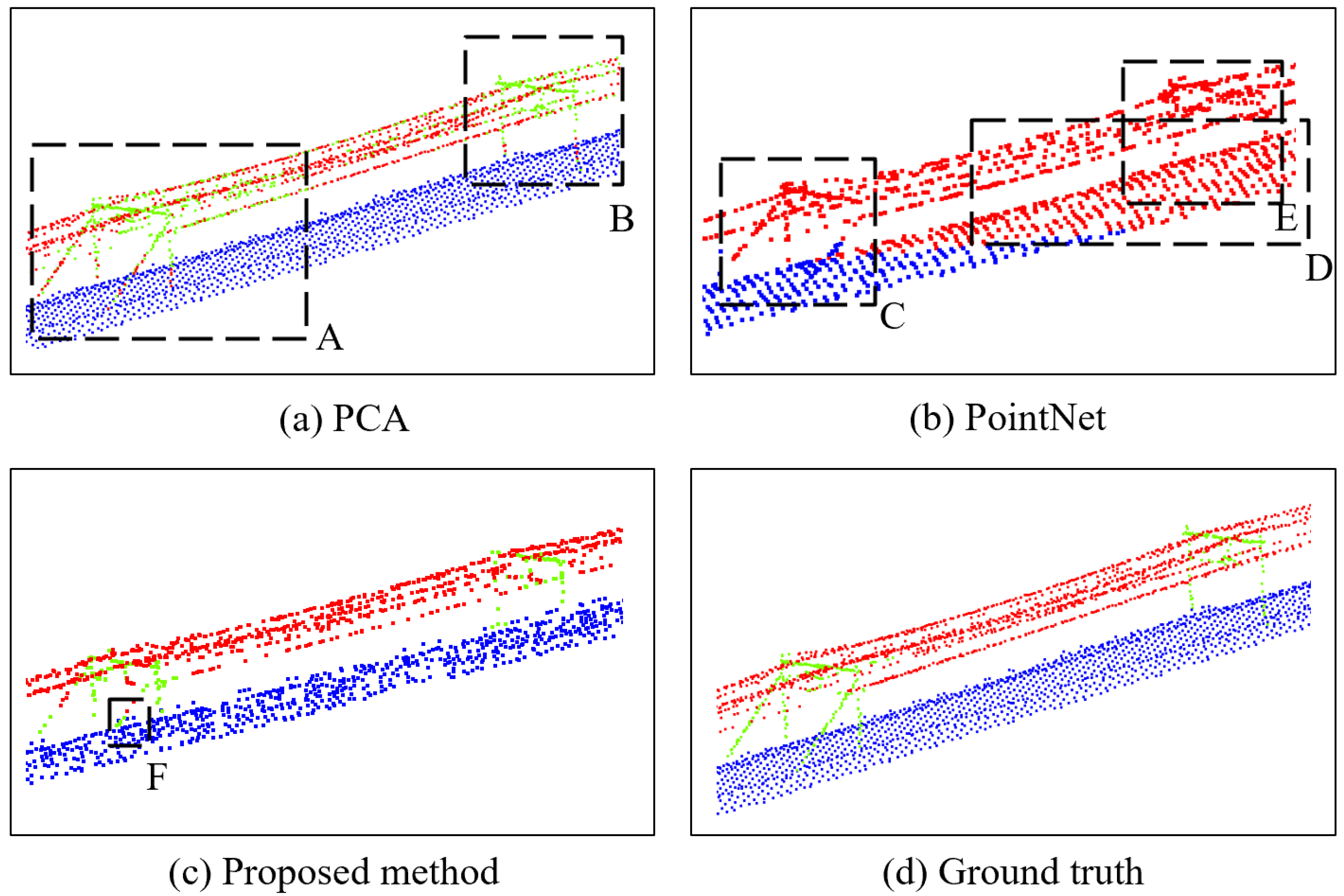
Remotesensing 14 05272 g016
Figure 17. The results of different wire segmentation methods. The wire, pylon, and ground are colored with red, green, and blue, respectively. The black dotted frame indicates points that are classified with error.
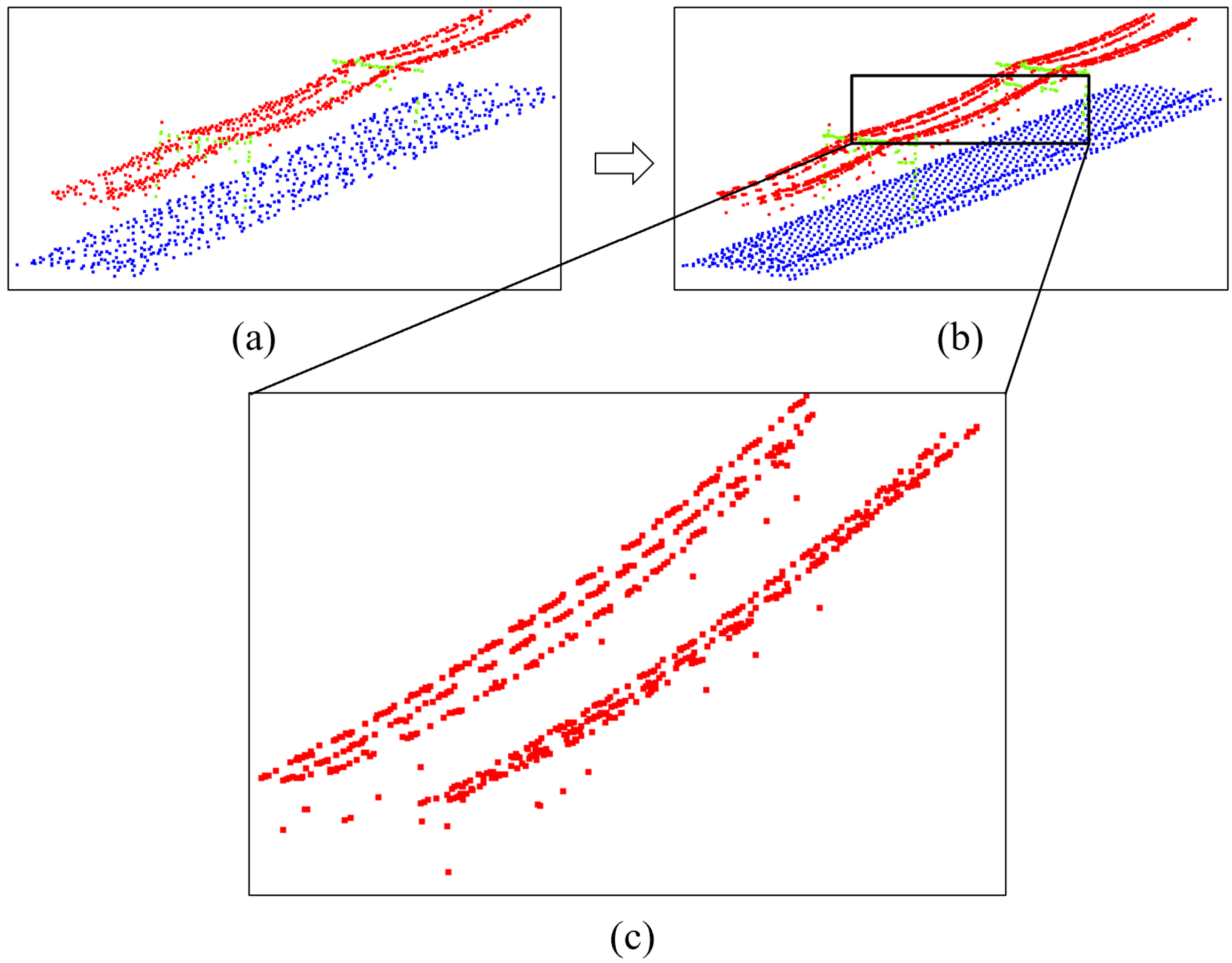
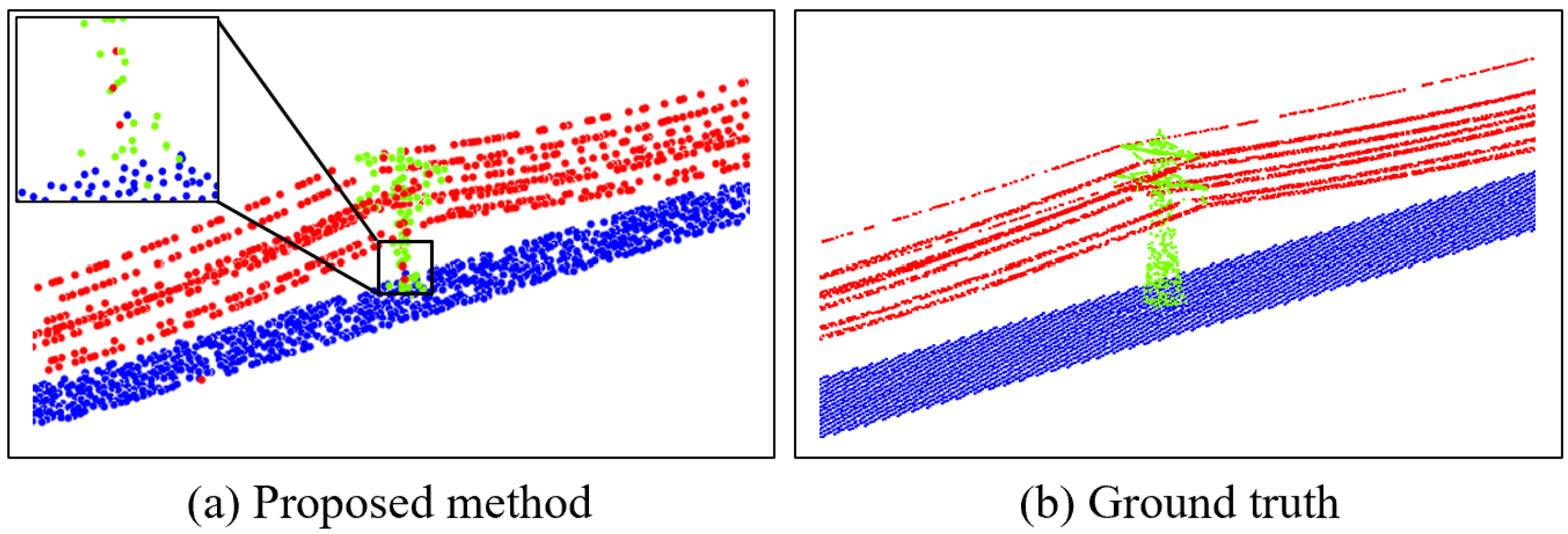
Remotesensing 14 05272 g017
Figure 18. Raw wire reverse mapping and span extraction. (a) wire point cloud after segmentation by the proposed model; (b) wire segmentation results of the original dataset after reverse mapping; (c) span extraction results.
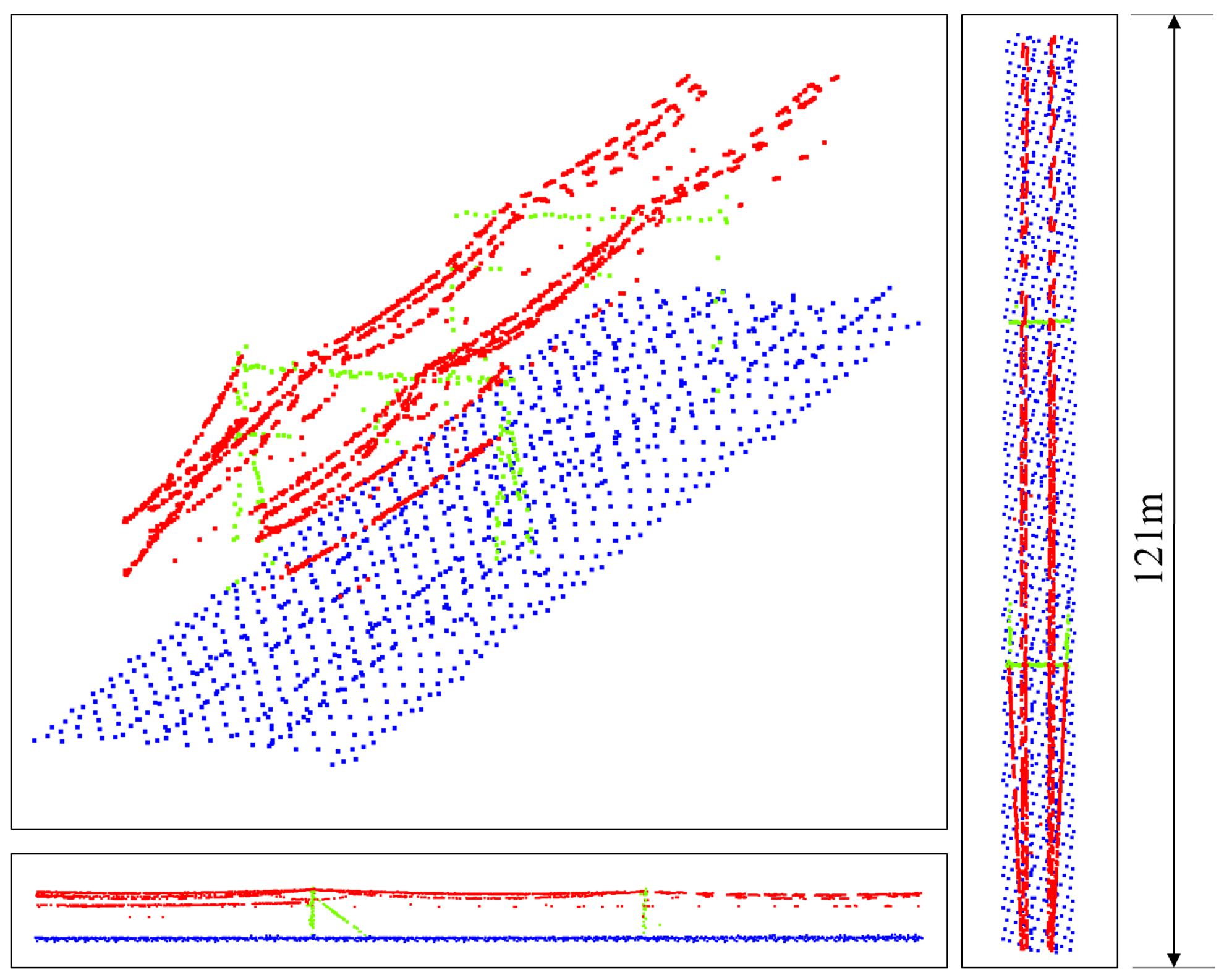
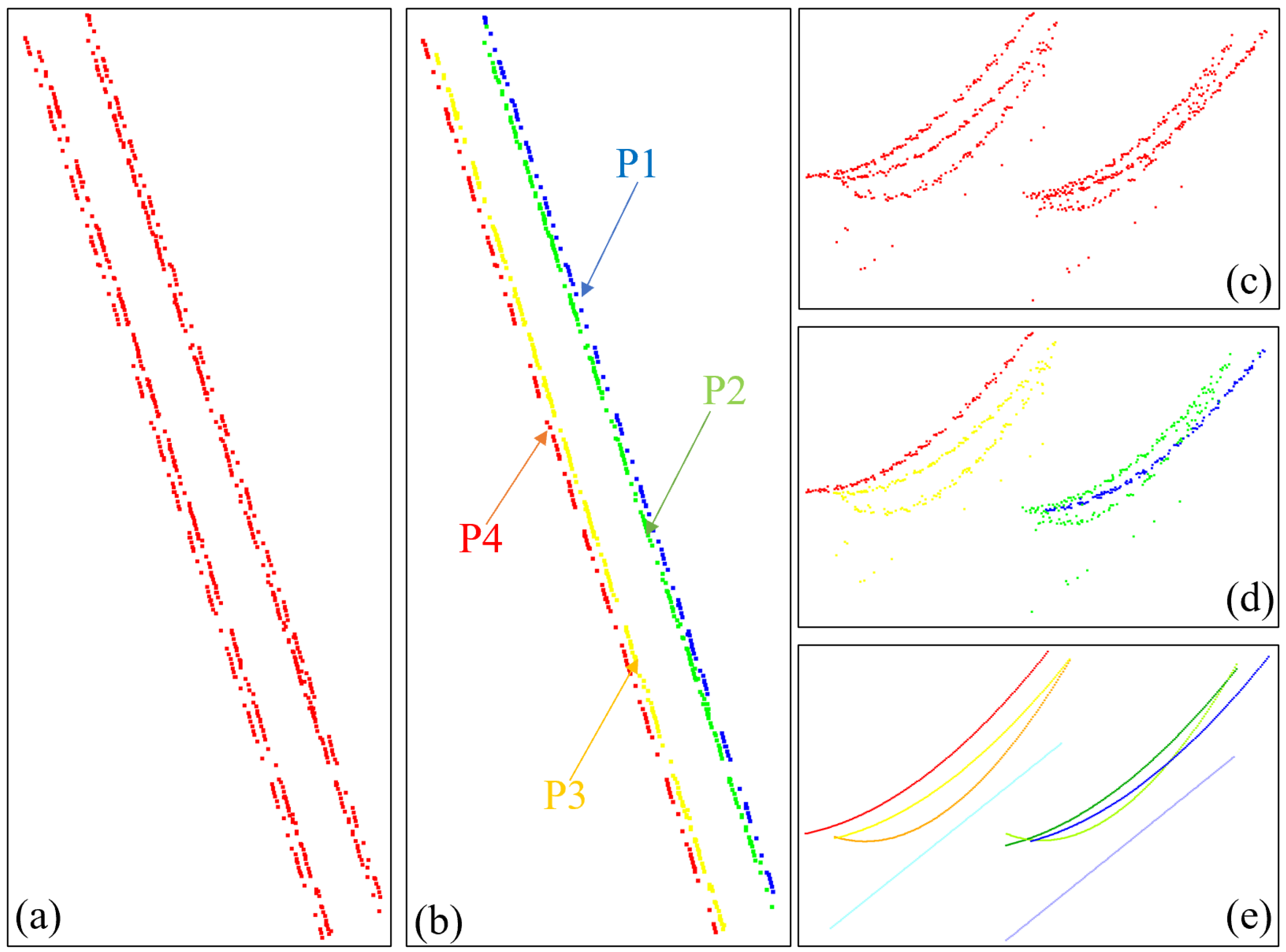
Remotesensing 14 05272 g018
Figure 19. Wire individualization and reconstruction. (a) wire points distribution on the XOY plane; (b) wire individualization based on the XOY plane; (c) side view of (a); (d) side view of (b); (e) wire reconstruction results.
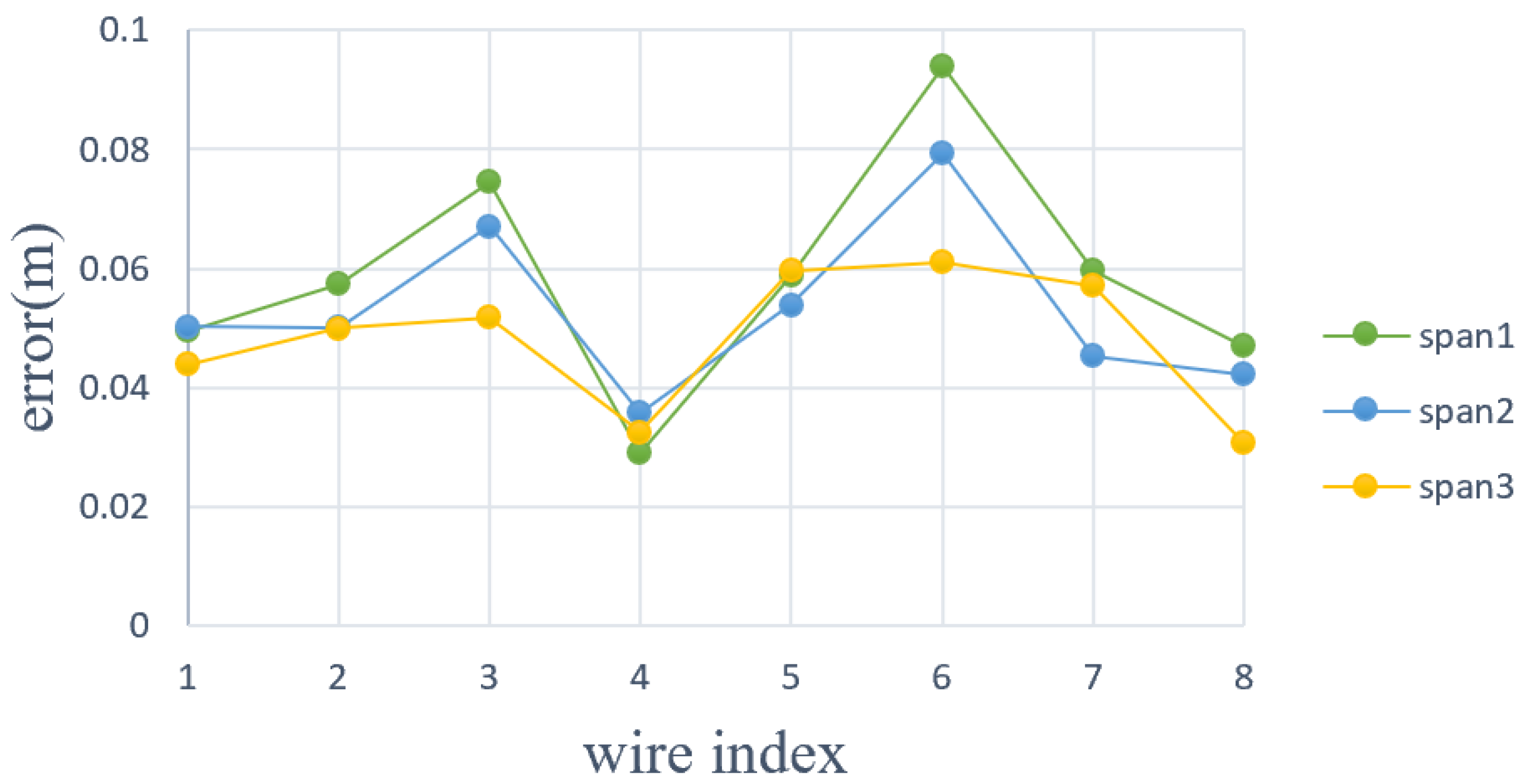
Remotesensing 14 05272 g019
Figure 20. Fitting error for eight wires at each span.
Remotesensing 14 05272 g020
Figure 21. (a) High-voltage powerline scenario; (b) pre-processing result.
Remotesensing 14 05272 g021
Figure 22. The results of proposed powerline segmentation methods. The powerline, pylon, and ground are colored with red, green, and blue, respectively. The black dotted frame indicates points that are classified by error.
Remotesensing 14 05272 g022
Table 1. Summary of powerline extraction methods.
MethodsDataCharacteristic
Model fitting based methodsMelzer and Briese [25]ALSIteratively bottom-up HT strategy
Jing et al. [26]ALSLSM-Based line fitting
Sohn et al. [27]ALSIntegrated HT, eigenvectors, and point density
Yadav and Chousalkar [28]MLSHT-based powerline extraction
Lehtomäki et al. [29]MLSVoxelization, PCA and RANSAC
Clustering based methodsCheng et al. [33]MLSBottom-up clustering
Guan et al. [34]MLSIntegrates height filters, spatial density filters, size and shape filters
Liang et al. [35]ALSEuclidean distance-based clustering
Machine Learning based methodsGuo et al. [36]ALSJoint-Boost classification using 26 features
Wang et al. [37]ALSSVM-based extraction
Peng et al. [38]ALSRF-based classification
Li et al. [23]ALSGraph convolution-based identification
Proposed methodALSDeep learning based method for extraction and RANSAC based wire fitting
Table 2. Descriptions of the dataset.
ParametersValue
Length(km)7
Number of points (million)0.18
Density ( pts / m 2 )15
Number of pylons106
Table 3. Specifications of the experimental environment.
Experiment EnvironmentConfigurations
Operating SystemUbuntu20.04
CPUInter®Xeon(R)Silver 4210R CPU@2.40GHZ×40
GPUNVIDIA Corporation GV100[TITAN V]
RAM64GB
VRAM12GB
Deep Learning PlatformPyTorch
PythonPython3.6
Table 4. Parameter settings.
PartParameterValue
Pre-processingsegment standard (contain pylon numbers)2
rotation amplification3 times
training data392 tiles
Segmentationmoment estimation0.9
learning rate0.001
batch size40
epoch200
R4 m
k3
Reconstruction σ 0.15 m
t50 times
Table 5. Comparison of the number of various targets in the original data and after downsampling.
DatasetRaw Point CloudsDownsampled Results
LinePylonGroundTotalLinePylonGroundTotal
156415414,65515,37356415422042922
2146563728,02130,123146563745436645
392141918,74520,08592141913952735
Table 6. Comparison of the MIoU and ACC of the three different wire segmentation methods.
DatasetPCAPointNetProposed Method
MIoUACCMIoUACCMIoUACC
Railway0.60290.84380.44600.73940.82650.9689
Table 7. The performance of different modules proposed in this work in aspects of MIoU and ACC.
DatasetPointNetPointNet+GFEPointNet+GFE+NIAPointNet(C)+GFE+NIA
MIoUACCMIoUACCMIoUACCMIoUACC
Railway0.44600.73940.80120.96130.81230.96530.82650.9689
Table 8. Fitting rate and fitting error of the railway overhead wires at each span.
Data SetRaw PointsFit PointsFitting Rate (%)Fitting Error (m)
span169366796.240.058
span270568196.590.052
span365863296.040.048
average68566096.310.053
Table 9. MIoU and ACC of the proposed method in a high-voltage powerline scenario.
DatasetProposed Method
MIoUACC
High-voltage0.89940.9852
Publisher’s Note: MDPI stays neutral with regard to jurisdictional claims in published maps and institutional affiliations.

