LiDAR Odometry and Mapping Based on Neighborhood Information Constraints for Rugged Terrain

Abstract

The simultaneous localization and mapping (SLAM) method estimates vehicles’ pose and builds maps established on the collection of environmental information primarily through sensors such as LiDAR and cameras. Compared to the camera-based SLAM, the LiDAR-based SLAM is more geared to complicated environments and is not susceptible to weather and illumination, which has increasingly become a hot topic in autonomous driving. However, there has been relatively little research on the LiDAR-based SLAM algorithm in rugged scenes. The following two issues remain unsolved: on the one hand, the small overlap area of two adjacent point clouds results in insufficient valuable features that can be extracted; on the other hand, the conventional feature matching method does not take point cloud pitching into account, which frequently results in matching failure. Hence, a LiDAR SLAM algorithm based on neighborhood information constraints (LoNiC) for rugged terrain is proposed in this study. Firstly, we obtain the feature points with surface information using the distribution of the normal vector angles in the neighborhood and extract features with discrimination through the local surface information of the point cloud, to improve the describing ability of feature points in rugged scenes. Secondly, we provide a multi-scale constraint description based on point cloud curvature, normal vector angle, and Euclidean distance to enhance the algorithm’s discrimination of the differences between feature points and prevent mis-registration. Subsequently, in order to lessen the impact of the initial pose value on the precision of point cloud registration, we introduce the dynamic iteration factor to the registration process and modify the corresponding relationship of the matching point pairs by adjusting the distance and angle thresholds. Finally, the verification based on the KITTI and JLU campus datasets verifies that the proposed algorithm significantly improves the accuracy of mapping. Specifically in rugged scenes, the mean relative translation error is 0.0173%, and the mean relative rotation error is 2.8744°/m, reaching the current level of the state of the art (SOTA) method.

1. Introduction

The key technologies of unmanned navigation include environment perception, mapping, localization, decision making, and planning [1,2]. As shown in Figure 1, SLAM methods can estimate the pose of robots and unmanned ground vehicles in an unknown environment, and construct 3D maps to provide significant priori information for the navigation of unmanned systems. Consequently, they play an important role in the field of autonomous driving and unmanned ground vehicles. The sensors commonly used in SLAM methods are cameras and LiDAR in the current research. However, the data provided by the camera are two-dimensional images, which lack depth information and suffer from scale ambiguity and illumination variation, resulting in inaccurate representation of texture information. Therefore, the method based on a visual sensor is only suitable for low precision localization and mapping. The data provided by LiDAR are three-dimensional point clouds, which are not affected by light variations, resulting in the LiDAR-based SLAM method becoming a hot research topic in recent years. The three primary components of the LiDAR-based SLAM method include front-end odometry, loop closure detection, and back-end optimization. Firstly, front-end odometry is performed using the interframe matching algorithm based on the point cloud information from LiDAR so as to estimate its pose and trajectory. Secondly, loop closure detection is intended to eliminate the cumulative error during the process of interframe matching by determining whether to reach the revisited place and estimating the pose between the current data and the historical data. Finally, back-end optimization globally optimizes the estimated pose and trajectory obtained by the odometry and closure detection is carried out, along with global pose and mapping for the point cloud.

The precision of pose estimation directly determines the effect of subsequent mapping. However, the existing pose estimation algorithms rely on the assumption of structural road and near-linearity motion, which still face significant challenges in complex scenes. Pose estimation algorithms are divided into two types: matching-based and feature-based. The matching-based pose estimation method adopts the geometric registration technique as a foundation, of which the Iterative Closest Point (ICP) algorithm proposed by Besl et al. [3] is a classic example. The ICP algorithm directly matches the point cloud and constructs constraints on neighborhood information by minimizing the Euclidean distance residuals of two adjacent point clouds to be matched to estimate pose change. However, there are also some restrictions on this algorithm. For instance, in view of the fact that the single distance constraint cannot accurately identify the differences between the feature points of adjacent frames, and the number of scanned point set elements is huge, this algorithm will produce mis-registration or even matching failure. Additionally, since the algorithm is sensitive to the initial pose, its precision will affect the subsequent registration precision. Some ICP variants have been proposed to address the aforementioned issues such as point-to-plane ICP [4] and generalized ICP (GICP) [5]. However, these methods convert the point-to-point matching problem into point-to-plane and plane-to-plane matching, but fail to change the problem caused by inaccurate initial values in essence. In addition, some factors such as noise and outlier cloud will also affect the accuracy of registration [6].

The feature-based pose estimation method extracts feature points by abstracting the geometric primitives of point clouds, such as points, lines, and planes, reducing the number of point clouds involved in pose estimation. LiDAR Odometry and Mapping (LOAM) [7] adopts a feature-based method in the pose estimation, where the edge and planar points are extracted according to the roughness of the local region of point cloud data, and different features are registered separately to reduce the mis-registration of feature point pairs. However, the aforementioned method is generally based on the assumption of structural and flat roads. When facing rugged terrain, the overlapping area of adjacent frames is reduced. Vehicles undulate with the ground in rugged road conditions, resulting in sensor data acquisition being unparallel. In that case, the adjacent frame data collected by a rugged road creates a new angle offset in the vertical direction compared with the adjacent frame data collected by a smooth road. Thus, it is a new challenge to extract a certain number of valuable edge points and surface points from the above adjacent frame data. At the same time, the relative position between the matching point pairs alters as a result of the changes in the pitching of the vehicles due to the roadways’ undulations. In this case, it is challenging to distinguish the difference between the point cloud data of adjacent frames and ensure the correspondence between the feature points when depending solely on the distance information constraints. In order to solve the registration error problem brought on by roadway undulations in rugged terrains, Lightweight and Ground-Optimized LiDAR Odometry and Mapping (LeGO-LOAM) [8] has established a ground constraint filtering interference feature to enhance feature points’ description of rugged scenes. However, the essence of this method still lies in the utilization of a single distance information constraint to distinguish the difference between the point cloud data of adjacent frames.

In this paper, we present LoNiC, a SLAM algorithm based on neighborhood information constraints, to address the aforementioned issues brought on by the non-smooth motion of vehicles in rugged terrains. From our perspective, extracting valuable feature information through the SLAM algorithm to increase the describing ability of point cloud features in rugged scenes and improving the discrimination of point cloud data differences between adjacent frames by adding constraint information is crucial to promoting the algorithm’s overall performance in rugged scenes. Therefore, this paper first proposes a feature point extraction method based on surface information description. In this method, the normal vector angle in the local neighborhood is used to describe the fluctuation degree of the surface, followed by a dynamic adjustment of the neighborhood surface fluctuation thresholds in accordance with the relationship between the local and average surface fluctuation factors. The feature points with surface information are then screened using the above thresholds to describe rugged scenes. Then, a new multi-scale constraint relationship is constructed in this paper based on curvature, normal vector angle, and distance information to identify the difference between the point cloud data of adjacent frames so as to ensure the reliability of feature point correspondences. Finally, this paper proposes a point cloud registration method based on dynamic iteration factors to enhance the performance of the SLAM algorithm. In this method, the distance and angle thresholds are dynamically adjusted during each iteration, and the corresponding relationship of the matching point pairs is modified by dynamic iteration factors to reduce the dependence on the initial value in the registration process. The contributions of this study are as follows:

• A feature point extraction method based on surface information description is proposed, which effectively promotes the describing ability of point cloud features’ description of rugged scenes by extracting the features with high discriminability and value based on the differences in the point cloud neighborhood surface.
• A multi-scale constraint description method is proposed, which lessens the possibility of mis-registration and matching failure by integrating the surface information of the feature points, such as curvature and normal vector angle, as well as the distance information between the feature points to enhance the discrimination of the differences between the point cloud data of adjacent frames in rugged terrains.
• Dynamic iteration factors are introduced to the point cloud registration method, which reduce the dependence of the registration process on the initial pose by adjusting the thresholds of distance and angle in the iteration to modify the corresponding relationship of matching point pairs.
• A comprehensive evaluation of our solution is made over the KITTI sequences with a 64-beam LiDAR and the campus datasets of Jilin University collected by a 32-beam LiDAR, and the results demonstrate the validity of our proposed LCD method.

The remainder of this paper is structured as follows: Section 2 briefly covers the related work of this study. Section 3 demonstrates the simultaneous localization and mapping (SLAM) algorithm of the modified odometry based on the neighborhood information constraints. Section 4 displays the experiment results based on the KITTI and JLU datasets. Section 5 serves as a conclusion of this study.

2. Related Work

2.1. Traditional LiDAR-Based SLAM Method

The traditional LiDAR-based SLAM method is matching-based [9,10,11,12,13], employing a geometric registration technique for point cloud registration. Iterative Closest Point (ICP) and Normal Distributions Transform (NDT) are two common geometric registration algorithms.

The ICP algorithm, which was first proposed by Besl and Mckay [3], iteratively calculates the transformation matrix between the two point clouds to be matched by minimizing the Euclidean distance of them to obtain the relative pose and estimate the vehicle motion. Although the ICP algorithm is simple and easy to implement, it is sensitive to the initial pose value, and its calculation efficiency is relatively low, making it prone to local optimum. Therefore, many researchers have proposed modified algorithms and applied them to the odometry of the LiDAR-based SLAM method [14,15,16]. The point-to-plane ICP method replaces the point-to-point distance in the original ICP algorithm with the point-to-plane distance, which is more suitable for the case of low point cloud density and can lessen the dependence of ICP on the initial value. ElasticFusion [10] and Surfel-based Mapping (SuMa) [12] employ the point-to-plane ICP method in the odometry. GICP [5] introduced a Gaussian probability model to the ICP cost function to reduce the computational complexity, which can handle the problems at the point, line, and plane level flexibly, but requires additional stability processing. Koide et al. [11] adopted the GICP algorithm to construct the SLAM framework based on the pose graph.

Normal Distributions Transform (NDT) [17,18,19] is another standard geometric registration algorithm applied to the traditional LiDAR-based SLAM method. The two-dimensional NDT was first proposed by Biber [17] in 2003, and is used to obtain the point cloud pose to be registered by maximizing the possibility that the point to be registered is located on the reference (benchmark) scanning surface. Based on this, Magnusson [19] extended the two-dimensional NDT to three-dimensional matching. The essence of this method is to put the point cloud data into the grid composed of small cubes, convert the point cloud in each cube into a probability density function, and then calculate the matching relationship between the point clouds. The three-dimensional NDT algorithm has the advantages of a good initialization effect, fast running speed, and high robustness, and has been widely utilized in the LiDAR-based SLAM method. The NDT algorithm has been employed in the odometry of Hdl-Graph-SLAM [11] to propose a new SLAM method based on NDT and graph optimization, which can be applied to the extension of multi-sensor fusion. Erik et al. [20] described a graph-based SLAM method combining the NDT algorithm and occupancy mapping, which displays good mapping performance even in highly dynamic environments. Additionally, a proposed multi-scale NDT method has been proven to effectively improve the convergence properties of the algorithms [21]. Although the multi-scale method can provide accurate registration results when there is a large displacement between scans, the size and number of required scales are not always precise. Traditional LiDAR-based SLAM methods have great limitations due to the initial pose’s significant impact, which makes them vulnerable to the local optimum and weakens their robustness. Additionally, a solution must be found for the mis-registration caused by a large number of scanning point clouds.

2.2. LiDAR-Based SLAM Method for Rugged Scenes

Another LiDAR-based SLAM method is feature-based [7,8,22,23], which extracts feature points by abstracting geometric primitives, such as the points, lines, and planes of the point cloud, to reduce the number of point clouds participating in pose estimation. LOAM [7] is a typical feature-based LiDAR SLAM method, which extracts planar and edge points by calculating the roughness of the local region as an index to extract the feature information of the current frame instead of utilizing the whole point cloud data, thus reducing the computational overhead caused by the huge number of point clouds. As an extension of the LOAM framework, F-LOAM [24] adopts a non-iterative two-stage distortion correction method to replace the iterative distortion correction method with low computational efficiency, which improves the real-time performance of the algorithm. These two methods are both realized by extracting edge and planar features for registration. However, the roadway undulations in rugged terrains lead to the reduction in the describing ability of the original algorithm in the scenes. Thus, the precision of point cloud registration needs to be improved.

The most relevant works in this paper are LeGO-LOAM, SA-LOAM, and Semantic LiDAR Odometry and Mapping (SLOAM). As a new framework derived from LOAM, LeGO-LOAM [8] adds the segmentation processing function and establishes a ground constraint in an attempt to improve the registration precision of point clouds in rugged scenes. The essence of the LeGO-LOAM method is to achieve registration by identifying the difference between the point clouds of adjacent data frames using distance information constraints and determining the corresponding relationship of feature points. However, in rugged scenes, the relative positional relationship between feature point pairs is no longer consistent with the assumption under structural roads, and the single distance constraint cannot identify the differences between point clouds reasonably or determine the corresponding relationship of the feature points. SA-LOAM [25] employs semantic constraint plane fitting during registration to reduce mis-registration points and thus obtain more precise matching results for rugged terrains. Notably, the SA-LOAM method eliminates some effective feature points inevitably while filtering interference features, which leads to feature loss to a certain extent. Additionally, the universality of deep learning methods has certain limitations, as they need to be retrained once applied to a new scene. Considering the situations of high leaf occlusion in the rugged mountain forests, SLOAM [26] extracts good landmark features, such as tree branches and ground plane, through segmentation and instance detection to estimate the motion pose and construct a more accurate map.

2.3. LiDAR-Based SLAM Method for Rugged Scenes

In view of the SLAM mapping in different scenes, the JLUROBOT team conducted this study from the following two aspects. Firstly, some all-terrain data collection platforms were established for data tasks under different terrains. Figure 2 demonstrates some data collection platforms designed by the team, of which J5 is used for mountain forest scenes, Avenger is used for off-road scenes, and Volkswagen Tiguan is mainly used for structural roads. Secondly, the team designed and implemented SLAM algorithms for different scenes, and the LoNiC algorithm in this paper was designed for rugged terrains. Extracting valuable features and imposing reasonable constraints for matching point pairs are of great significance in constructing more effective maps for rugged terrains. On the one hand, valuable feature points exhibit strong discrimination, which facilitates the precise description of the scene in complex and bumpy terrains. On the other hand, a reasonable constraint can increase the discriminability of the differences between the feature points of adjacent frames and help select the matching point pairs with stronger correspondence from the feature points. Therefore, this paper proposed a LoNiC algorithm based on the previous findings.

3. Materials and Methods

3.1. Algorithm Overview

We introduce the LoNiC algorithm in this section. According to the flow in Figure 3, the algorithm is divided into LiDAR Odometry and Pose Graph Optimizer. The LiDAR Odometry estimates the vehicle pose change through the input data of point clouds, that is, register the point cloud at the current time point with that at the previous time point to calculate the relative position change in the two data frames. First, the extraction module for feature points described by surface information performs voxelized downsampling on the input point cloud, and adaptively filters the feature points with surface information according to the local surface fluctuation degree. Finally, the matching point pairs are sent to the registration module with dynamic iteration factors. The dynamic iteration factor is adjusted continuously in the iterative process to correct the correspondence of the matching point pairs to output the final pose estimation. Pose Graph Optimizer serves as a back-end optimization, and the factor graph is employed for global pose optimization in this paper, which is the same as the optimization strategy used in the LIO-SAM [23] method. The node information of the factor graph is provided by the LiDAR Odometry and loop closure detection (LCD) algorithm. The LCD algorithm selects all point cloud frames within a radius of 15 m from the current position in the historical data as loop closure candidate frames according to the GNSS data output by the Inertial Navigation System (INS). The candidate frames are then matched with the current point cloud frames, and the corresponding results are used for graph optimization.

3.2. Extraction Module for Feature Points Described by Surface Information

Since the huge amount of original point cloud data collected by LiDAR will affect the speed of subsequent registration, it is necessary to reduce the amount of three-dimensional point cloud data while maintaining the original features. Therefore, the method of downsampling the barycenter adjacent points based on voxel grids is utilized to reduce the collected data. Specifically, tiny three-dimensional spatial cubes called voxel grids are first created in the point cloud data, followed by replacing all the points in each voxel grid with the adjacent points of the barycenter. This downsampling method improves the processing speed of subsequent algorithms while keeping the original feature information. In order to extract the feature points with surface information for subsequent matching, we first use the normal vector and curvature of the point cloud to construct its surface features, followed by an adaptive extraction of the feature points described by the surface information according to the degree of surface fluctuation. Figure 4 is the algorithm flow diagram of this module.

3.2.1. Surface Feature Construction

In this paper, we perform the odometry registration based on surface features to estimate the pose transformation of point clouds. Since the distribution of the plane normal vector in the point cloud can characterize the local structure of the region, we construct the surface features of point cloud by calculating the normal vector and the ratio of normal vectors’ eigenvalues (curvature). In this paper, Principal Components Analysis (PCA) is used to obtain the normal vector for two main reasons: firstly, PCA is a common dimensionality reduction method. Through this method, the features of the plane fitted from the local point set can be reconstructed. The redundancy information of the original 3D data is eliminated and the data volume is reduced. Secondly, the relationship between the normal vector and the plane is vertical, which is exactly the eigenvector corresponding to the smallest eigenvalue of the three dimensions in the PCA process, thus reducing the processing steps. We suppose that the point set formed by all points in the neighborhood of any point $p_i$ in the point cloud set$P$is $C=\left\{p_{i1},p_{i2},\dots ,p_{ik}\right\}$. In order to obtain the normal vector estimation of point $p_i$, we first calculate the covariance matrix of the neighborhood $C$ to obtain the eigenvalue, and then find the feature vector corresponding to the smallest eigenvalue, which is the corresponding normal vector at the point $p_i$. The calculation process of normal vector is as follows

$$E_i=\frac{1}{k}{\displaystyle \sum }_{j=1}^k\left(p_{ij}-{\overline{p}}_i\right)\ast {\left(p_{ij}-{\overline{p}}_i\right)}^T,$$

(1)

$$E_i{v}_i={\lambda }_i{v}_i,$$

(2)

where $E_{i }$refers to the neighborhood covariance matrix of$p_i$. $k$ refers to the number of points in the point set$C$. $v_i$and${\lambda }_i$refer to the feature vector and eigenvalue of $E_{i }$to be obtained, respectively. ${\overline{p}}_i$refers to the center of the point set$C$, which can be calculated by the following formula

$${\overline{p}}_i=\frac{1}{k}{\displaystyle \sum }_{j=1}^k{p}_{ij}.$$

(3)

The selection of normal vectors needs to be determined by eigenvalues${\lambda }_i$, and we take the feature vector corresponding to the smallest eigenvalue as the normal vector.${\lambda }_i$contains three dimensions:${\lambda }_{i1}$, ${\lambda }_{i2}$, and ${\lambda }_{i3}$. Sort the feature value ${\lambda }_i$, if ${\lambda }_{i1}<{\lambda }_{i2}<{\lambda }_{i3}$, the direction of the feature vector $v_{i1 }$corresponding to${\lambda }_{i1}$is the direction in which the degree of dispersion of the neighborhood data of the point$p_i$ is the smallest, and is also the direction of the normal vector of the local neighborhood of the point$p_i$. In order to ensure the consistency of the direction of the normal vector and increase the precision of subsequent matching, we specify that the direction of the normal vector is consistent with the positive direction of the $z$-axis. The direction of the normal vector can be unified by Equation (4)

$$n_i=\{\begin{array}{c}\frac{v_i}{\Vert v_i\Vert },\frac{v_i}{\Vert v_i\Vert }.z>0\\ -\frac{v_i}{\Vert v_i\Vert },\frac{v_i}{\Vert v_i\Vert }.z<0\end{array},$$

(4)

where $z$ is the unit vector along the z-axis. The normal vector $n_i$ at $p_i$ can be obtained through the unitization of the feature vector$v_{i1}$. The eigenvalue ${\lambda }_{i1}$, ${\lambda }_{i2}$, and ${\lambda }_{i3}$ can be obtained according to the covariance matrix, whose size can be expressed by the length of the three semi-major axes of three-dimensional ellipsoid. When ${\lambda }_{i1}$ is equal to ${\lambda }_{i2}$ and ${\lambda }_{i3}$, the surface fluctuation of the local neighborhood of $p_i$is the largest, which is a spherical surface. When ${\lambda }_{i1}$ is much smaller than ${\lambda }_{i2}$ and ${\lambda }_{i3}$, the surface of the local neighborhood of $p_i$ is flat and approximates a plane, as shown in Figure 5. Therefore, the surface curvature at point $p_i$ can be calculated as follows.

$$\epsilon \left(p_i\right)=\frac{{\lambda }_{i1}}{{\lambda }_{i1}+{\lambda }_{i2}+{\lambda }_{i3}} .$$

(5)

3.2.2. Adaptive Extraction of Feature Points

An adaptive method of extracting feature points is proposed in this paper, and the angle distribution of normal vectors in the local neighborhood is employed to describe the fluctuation degree of the surface. The more scattered the angle distribution, the smaller the surface fluctuation in the point cloud region, the less need for feature points for description, and the fewer feature points need to be sampled in the region; in contrast, the more dispersed the angle distribution, the more obvious the surface fluctuation in the region, and the more feature points need to be extracted for description. Therefore, the threshold value needs to change dynamically with the fluctuation degree of the local surface. The angle $\theta \left(p_i\right)$ between a point $p_i$ of the point cloud and its normal vector in the neighborhood can be defined as

$$\theta \left(p_i\right)=\frac{1}{k}{\displaystyle \sum }_{j=1}^k{\theta }_{ij},$$

(6)

where${\theta }_{ij}$refers to the angle between the normal vector of$p_{i }$and the normal vector of the $j$th point in the neighborhood $k$. As shown in Figure 6a, the normal vector angle of the point cloud in the local neighborhood is large, indicating that the region is relatively undulating. Conversely, the normal vector angle changes little, indicating that the region is relatively smooth, as shown in Figure 6b.

The normal vector angles of the points in the $p_i$ neighborhood satisfy the larger variance, the more dispersed the distribution of normal vector angles; the smaller the variance, the more concentrated the distribution. This meets the requirements of normal distribution. Thus, we assume the normal vector angles of the points in the $p_i$ neighborhood are normally distributed. The threshold ${\tau }_i$ can be expressed as

$${\tau }_i=\frac{1}{\sqrt{2\pi }\sigma k}{\displaystyle \sum }_{i=1}^k\theta \left(p_i\right)·exp(-\frac{{\left(\theta \left(p_i\right)-\mu \right)}^2}{2{\sigma }^2}),$$

(7)

where $\mu$ is the mean value of the normal vector angle of the points in the neighborhood $p_i$, and ${\sigma }^2$ is the variance. The corresponding calculation formula is as follows

$$\mu =\frac{1}{k}{\displaystyle \sum }_{i=1}^k\theta \left(p_i\right),$$

(8)

$${\sigma }^2=\frac{1}{k}{\displaystyle \sum }_{i=1}^k{\left(\theta \left(p_i\right)-\mu \right)}^2,$$

(9)

Equation (7) demonstrates that the larger the fluctuation degree of the surface in the local region, the smaller the threshold ${\tau }_i$, and more feature points are extracted, while the smoother the region, the larger the threshold ${\tau }_i$, and fewer feature points are extracted.

The feature points are extracted according to the point$p_{i }$and its normal vector angle in the neighborhood. When $\theta \left(p_i\right)$ > ${\tau }_i$, the fluctuation degree at $p_{\mathrm{i}}$ is relatively large, thus $p_i$ is defined as the feature point; when$\theta \left(p_i\right)$ < ${\tau }_i$, the local region at $p_i$ is rather smooth, thus $p_i$is defined as the non-feature point.

3.3. Matching Module of Multi-Scale Constraint Description

The pitching of the vehicles changes significantly in rugged terrains due to the non-smooth motion of mobile platforms, which means that the relative positional relationship between the point clouds in the overlapping region of adjacent frames no longer meets the assumption under structural road conditions. In this case, there will be mis-registration and non-convergence in iterative calculations if we continue to employ the distance information as the constraints to search the matching point pairs in two frame point clouds. In order to achieve precise registration of feature points in rugged scenes, this paper proposes a matching search mechanism of multi-scale constraint description. In the proposed mechanism, a new constraint description has been established based on curvature, normal vector angle, and distance, which can be used to search matching point pairs according to the similarity of the constraint description. The algorithm flow in this section is displayed in Figure 7.

We suppose that$Q$is the point cloud set of point cloud$P$, and $q_{i }$is the corresponding point of $p_{i }$ in $Q$. We employ KD-TREE to search the neighborhood $k$ of $p_{i }$ in the set$Q$, which are$q_{i1},q_{i2},\dots ,q_{ik}$. Hence, three binding terms can be defined:

The first binding term is the Euclidean distance ratio between feature points

$$s\left(p_i,q_{ij}\right)=\frac{d\left(p_i,q_{ij}\right)}{d\left(p_i,q_{ik}\right)},$$

(10)

where $d(*)$ is a function of distance.

The second binding term is the surface curvature ratio $c$ of feature points

$$c\left(p_i,q_{ij}\right)=\frac{\epsilon \left(q_{ij}\right)}{\epsilon \left(p_i\right)},$$

(11)

The third binding term is the ratio $e$ of normal vector angle of feature points

$$e\left(p_i,q_{ij}\right)=\frac{\theta \left(q_{ij}\right)}{\theta \left(p_i\right)},$$

(12)

For the points in the neighborhood $k$, a new constraint relationship is constructed according to the three binding terms, and the similarity scores are calculated

$$score\left(q_{ij}\right)=\alpha s\left(p_i,q_{ij}\right)+\beta c\left(p_i,q_{ij}\right)+\gamma e\left(p_i,q_{ij}\right),$$

(13)

where $\alpha ,\beta ,\gamma$refer to the coefficients, which conform to the following relationship

$$\alpha +\beta +\gamma =1$$

(14)

The point $q_j$ with the highest score is the corresponding point of $p_i$. $p_i$ and $q_j$ are defined as a matching point pair.

3.4. Registration Module with Dynamic Iteration Factors

The dynamic iteration factor is introduced for registration in this paper, and the algorithm flow of this module is shown in Figure 8. In the registration iteration, the matching between the initial point cloud and the target point cloud becomes more precise every time the ICP algorithm completes one iteration, which means that the offset angle and distance between the point cloud and its matching point cloud become smaller, as shown in Figure 9. Therefore, the iteration factors of dynamic angle and dynamic distance are combined in this paper to compress the scale, correct the corresponding relationship of ICP matching point pairs, and solve the local optimum of registration caused by inaccurate initial values.

We need to convert the matching point cloud $Q$ into the coordinate system of $P$, and calculate the coordinate transformation parameters $R$ (rotation matrix) and $T$ (translation vector). When $Q$ and $P$ undergo continuous rotation and translation, the error functions are minimized and the corresponding registration effect is optimal. The rotation translation error $E\left(p_i,q_j\right)$ is expressed as

$$E\left(p_i,q_{ij}\right)=\frac{1}{2}\Vert \left(R{p}_i+T\right)-q_j\Vert {}^2$$

(15)

The cosine value of the normal vector angle between the matching point pairs is taken as the angle error equation of the matching point pairs

$$\cos \theta =\frac{n_i.n_j}{\Vert n_i\Vert \ast \Vert n_j\Vert }.$$

(16)

where $n_i$ and $n_{ij}$ refer to the normal vector of the point $p_i$ and $q_j$, respectively. $\theta$ refers to the normal vector angle between two matching point pairs.

The weight of the matching point pairs can be calculated using Equation (17):

$$\left(p_i,q_j\right)=\{\begin{array}{c}1,(\cos \theta >Z,d\left(p_i,q_j\right)<S)\\ 0, \left(\mathrm{otherwise}\right)\end{array} ,$$

(17)

where $Z$ refers to the threshold of dynamic angle iteration. $S$ refers to the threshold of dynamic distance iteration. $m$ refers to the number of matching point pairs, which can be calculated by Equation (18):

$$m={\displaystyle \sum }_j{\displaystyle \sum }_{i}w\left(p_i,q_j\right),$$

(18)

The final error equation can be expressed as

$$I=\frac{{\displaystyle {{\displaystyle \sum }}_j}{\displaystyle {{\displaystyle \sum }}_i}\left[w\left(p_i,q_j\right)E\left(p_i,q_j\right)\right]}{m}.$$

(19)

Least square method can be employed to realize the minimization of Equation (19). After one iteration of the transformation matrix $H\left(R^{\prime },T^{\prime }\right)$, $Z$and $S$ can be updated by the following equation

$$Z^{new}=Z{D}_{dec},D_{dec}\in \left(0,1\right),$$

(20)

$$S^{new}=S{T}_{dec},T_{dec}\in \left(0,1\right),$$

(21)

where $D_{dec}$and $T_{dec}$refer to the angle and distance iteration coefficients, respectively.

After $I$ reaches the threshold by iterating for $t$ times, the ICP algorithm stops, and the final transformation matrix $H_t\left(R_t^{\prime },T_t^{\prime }\right)$ is obtained, which can be employed to transform the current frame to realize the global incremental mapping.

4. Experiments

This section will evaluate the proposed LoNiC method on the KITTI and JLU campus datasets and compare it to the popular LIO-SAM and LeGO-LOAM methods. The codes of the LIO-SAM and LeGO-LOAM algorithms can be downloaded from the developers’ website. The LoNiC, LIO-SAM, and LeGO-LOAM algorithms are all implemented in c++, and all the experiments in this paper were conducted on a computer with Ubuntu 18.04 operating system, an Intel X5675 CPU, and 16 GB memory.

4.1. Datasets

4.1.1. KITTI Dataset

KITTI [27] is a classic benchmark dataset, which is widely used in SLAM and three-dimensional object detection tasks. We utilized the data of 01, 02, 04, 05, 06, 07, 08, 09, and 10 in KITTI raw benchmark to evaluate the performance of the proposed method in this paper. The point cloud data of the KITTI dataset is obtained by Velodyne HDL-64E, and its ground truth data is obtained by Oxford RT3000. The number of data frames, trajectory length (m), and loop closure of each section used in the experiment are shown in

Table 1. Details of the KITTI dataset.

Sequence	01	02	04	05	06	07	08	09	10
Scans	1101	4661	271	2761	1101	1101	5171	1591	1201
Trajectory length (m)	2453	5067	393	2205	1232	694	3222	1705	919
Loop closure (Y/N)	N	N	N	Y	Y	Y	Y	Y	N

.

4.1.2. JLU Campus Dataset

In order to verify the method proposed in this paper, we collected data from four sections of rugged roads on the campus of Jilin University using the Volkswagen Tiguan as the mobile platform, using Velodyne HDL32E LiDAR to collect point cloud data in each section. We also employed the Inertial Navigation System NPOS220S to record the pose and position of each frame data. Velodyne HDL32E was placed on the aluminum frame of the roof center, and NPOS220S was placed in the trunk of the Tiguan. The data acquisition platform is shown in Figure 10, and the number of frames, trajectory length (m), and loop closure of each data section are shown in

Table 2. Details of the JLU campus dataset.

Sequence	JLU_062801	JLU_062802	JLU_070101	JLU_070102
Scans	3867	1648	7584	7779
Trajectory length (m)	754	382	1824	2044
Loop closure (Y/N)	N	N	Y	Y

.

4.2. Experimental Results and Analysis

In the experiment, the mean relative pose error (mRPE) was employed to evaluate the accuracy of the maps. mRPE includes two indexes: the mean relative translation error and the mean relative rotation error. The mean relative translation error reflects the displacement deviation between the constructed map and the ground truth in the horizontal direction. The mean relative rotation error reflects the angular deviation between the constructed map and the ground truth of the map in the vertical direction. To ensure the fairness of the comparison, all the performance and precision results shown in each experiment were averaged over three trials of playback of each dataset.

4.2.1. KITTI Dataset

Two experiments were run on the KITTI dataset to demonstrate the proposed LoNiC method’s efficacy in general scenarios. The first group of experiments was conducted to verify the effectiveness of the odometry method, and the second group verified the performance of the SLAM algorithm.

• Ablation Experiment

In order to verify the advantages of introducing constraints on neighborhood information into the odometry, we designed an odometry ablation experiment on the general KITTI dataset. Since the back-end part of LoNiC adopts the same strategy as LIO-SAM, a comparison of the proposed LoNiC method with the LIO-SAM was conducted. The major difference between LoNiC and LIO-SAM lies in their odometry. The LIO-SAM method divides the feature points into the edge and planar points and employs the distance information to constrain the registration, while the LoNiC method adopts the odometry method based on neighborhood information constraints, as discussed in Section 3.

Table 3. Relative pose error of LIO-SAM and LONIC on the KITTI dataset.

	Method	LIO-SAM	LoNiC
Sequence
01		3.4853/0.0069	2.3651/0.0041
02		1.9191/0.0054	2.1181/0.0057
04		1.4769/0.0049	1.2080/0.0043
05		0.6241/0.0037	0.6189/0.0038
06		12.3343/0.0348	12.3265/0.0336
07		0.5615/0.0040	0.7151/0.0059
08		3.5843/0.0136	4.4680/0.0163
09		1.9774/0.0063	1.4933/0.0049
10		1.5089/0.0068	1.4544/0.0065
Average		3.0524/0.0096	2.9742/0.0095

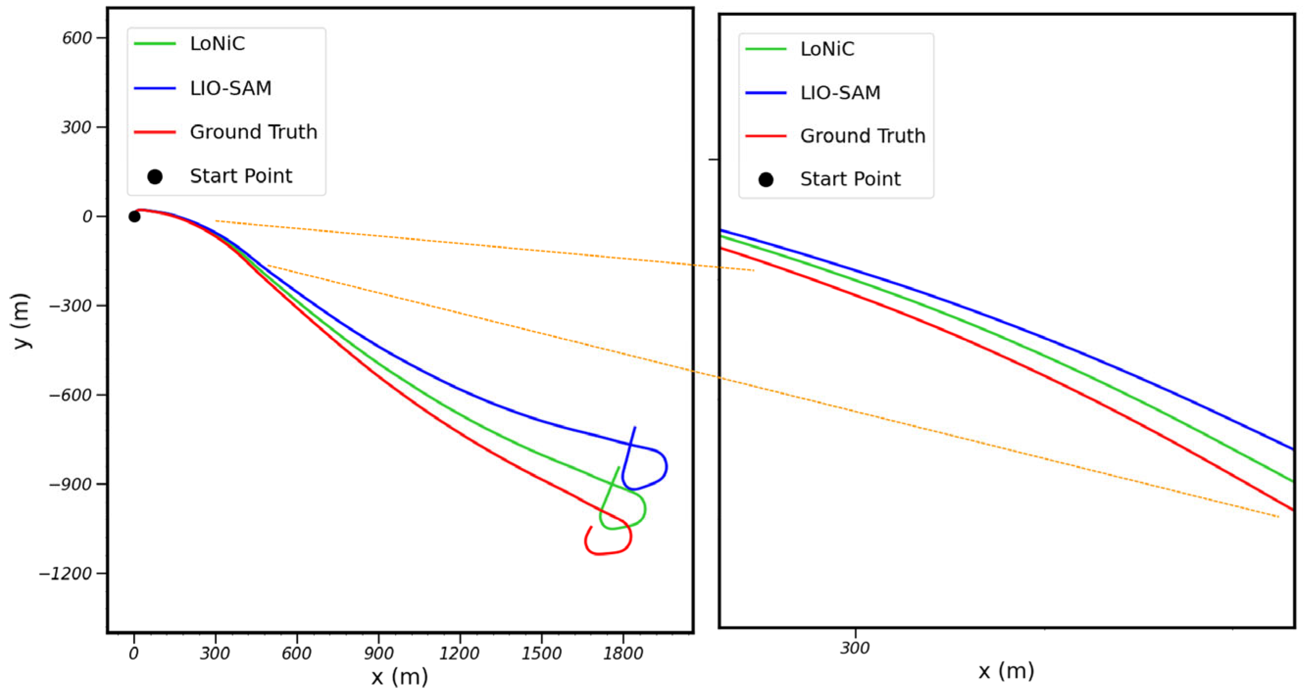
Note: Relative translation error (%)/relative rotation error (°/m). Bold numbers indicate the best performance.

exhibits the relative pose errors of LIO-SAM and LONIC on the KITTI dataset. As can be seen, the LoNiC method proposed outperforms the upper LIO-SAM on the KITTI dataset, especially in terms of mapping accuracy, which can reach the state of the art (SOTA) level. Specifically, the mean relative translation error and the mean relative rotation error of the LoNiC method on nine data sequences are 2.9742% and 0.0095°/m, which are 0.0782% and 0.0095°/m lower than that of the LIO-SAM method, respectively. Therefore, the mapping accuracy of the LoNiC method is better than that of the LIO-SAM method, especially in 01 and 09 sequences. 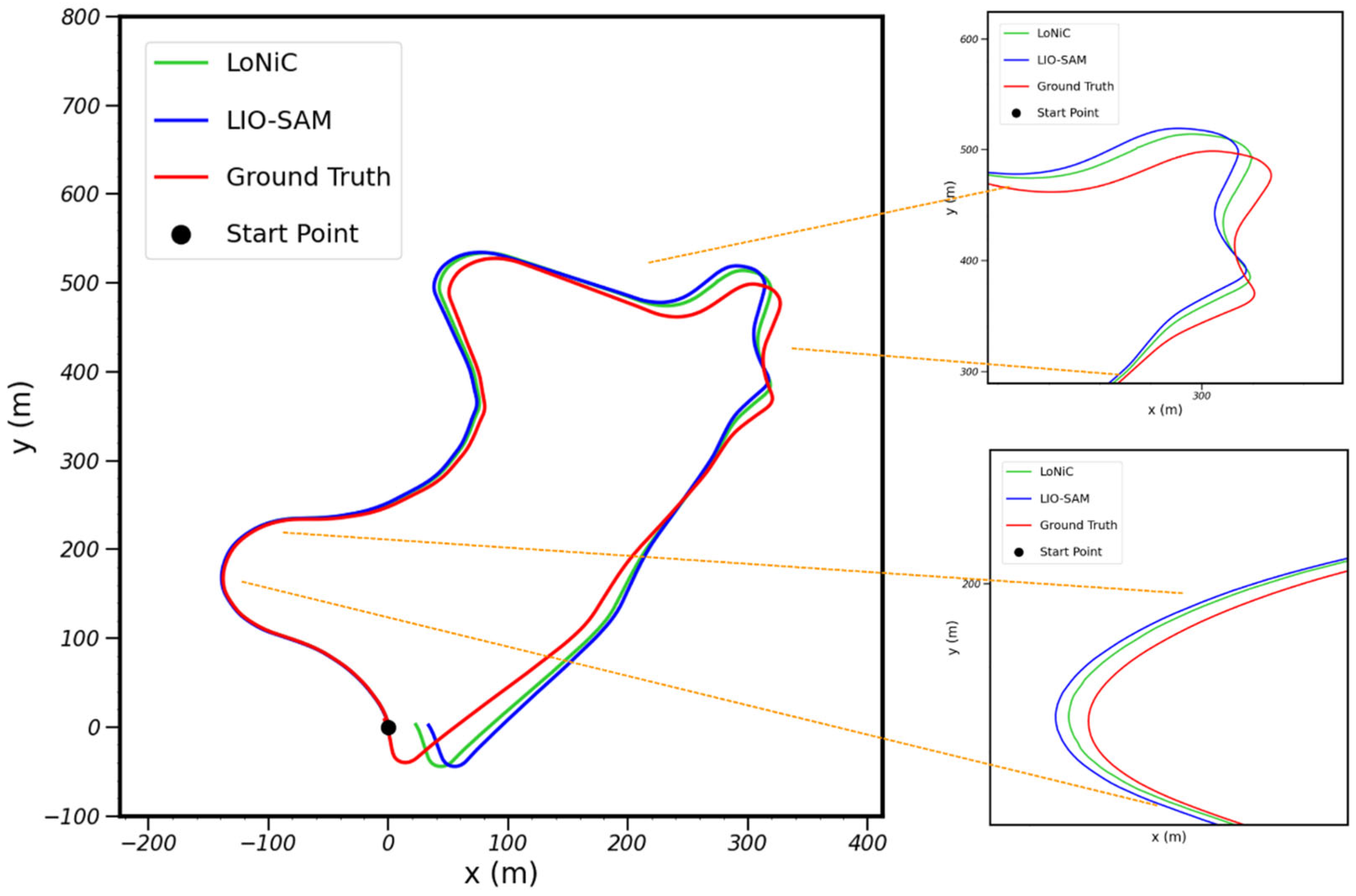According to the ground truth of sequence 01 in the KITTI dataset, the mapping trajectory of LIO-SAM and LoNiC displayed in Figure 11, the mapping trajectory of LoNiC is closer to the ground truth without loop optimization, indicating that the odometry of the LoNiC method is better than that of LIO-SAM, and the mapping results are more accurate. The feature points extracted by the odometry of LIO-SAM are more appropriate for the mapping of structured roads, while the description of complicated conditions exhibits unsatisfactory performance. Conversely, the proposed LoNiC obtains feature points with surface information with the angle distribution of neighborhood normal vectors, effectively illustrating the rugged terrain and raising the mapping accuracy. Similarly, according to the ground truth of sequence 09 in the KITTI dataset, the mapping trajectory of LIO-SAM, and the mapping trajectory of LoNiC displayed in Figure 12, the experimental results of the LoNiC method are better than those of LIO-SAM with loop closure detection (at the starting position). We analyzed the ground truth of these nine sections of data and found that the elevation fluctuation of the 01 and 09 sequences was more obvious than in other sequences. The result further demonstrates the effectiveness of the feature extraction scheme and constraint method proposed in this paper, which can lessen the mis-registration of feature points and improve the precision of the odometry.

2.

Comparative Experiment

This paper compared the proposed LoNiC with another SOTA method called LeGO-LOAM on the KITTI dataset to verify the mapping ability and effect of the LoNiC algorithm and evaluated the mapping results by using the mean relative pose error (mRPE).

According to

Table 4. Relative pose error of LeGO-LOAM and LONIC on the KITTI dataset.

	Method	LeGO-LOAM	LoNiC
Sequence
01		28.3265/0.0257	2.3651/0.0041
02		10.6081/0.0108	2.1181/0.0057
04		2.3260/0.0066	1.2080/0.0043
05		2.1959/0.0056	0.6189/0.0038
06		2.3439/0.0083	12.3265/0.0336
07		1.6979/0.0068	0.7151/0.0059
08		3.8719/0.0092	4.4680/0.0163
09		8.3678/0.0078	1.4933/0.0049
10		7.6577/0.0084	1.4544/0.0065
Average		7.4884/0.0099	2.9742/0.0095

Note: Relative translation error (%)/relative rotation error (°/m). Bold numbers indicate the best performance.

, the mean relative rotation error and mean relative translation error of LoNiC are significantly better than those of LeGO-LOAM in the nine sections of data except for the 06 and 08 sequences. The possible reason why the error of sequences 06 and 08 of LoNiC is slightly worse than that of LeGO-LOAM is that the clustering strategy in LeGO-LOAM provides extra label information in the process of point cloud registration. Additionally, a combination of features helps to obtain better results. The mean translation error of LeGO-LOAM on these nine sections of data is 7.4884%, which is 4.5142% lower than that of LoNiC, being 2.9741%; the mean rotation error of LeGO-LOAM is 0.0099°/m, while that of LoNiC is 0.0094°/m, which reduces by 4.04% compared with LeGO-LOAM. This result indicates that LoNiC can reduce the cumulative errors of mapping. 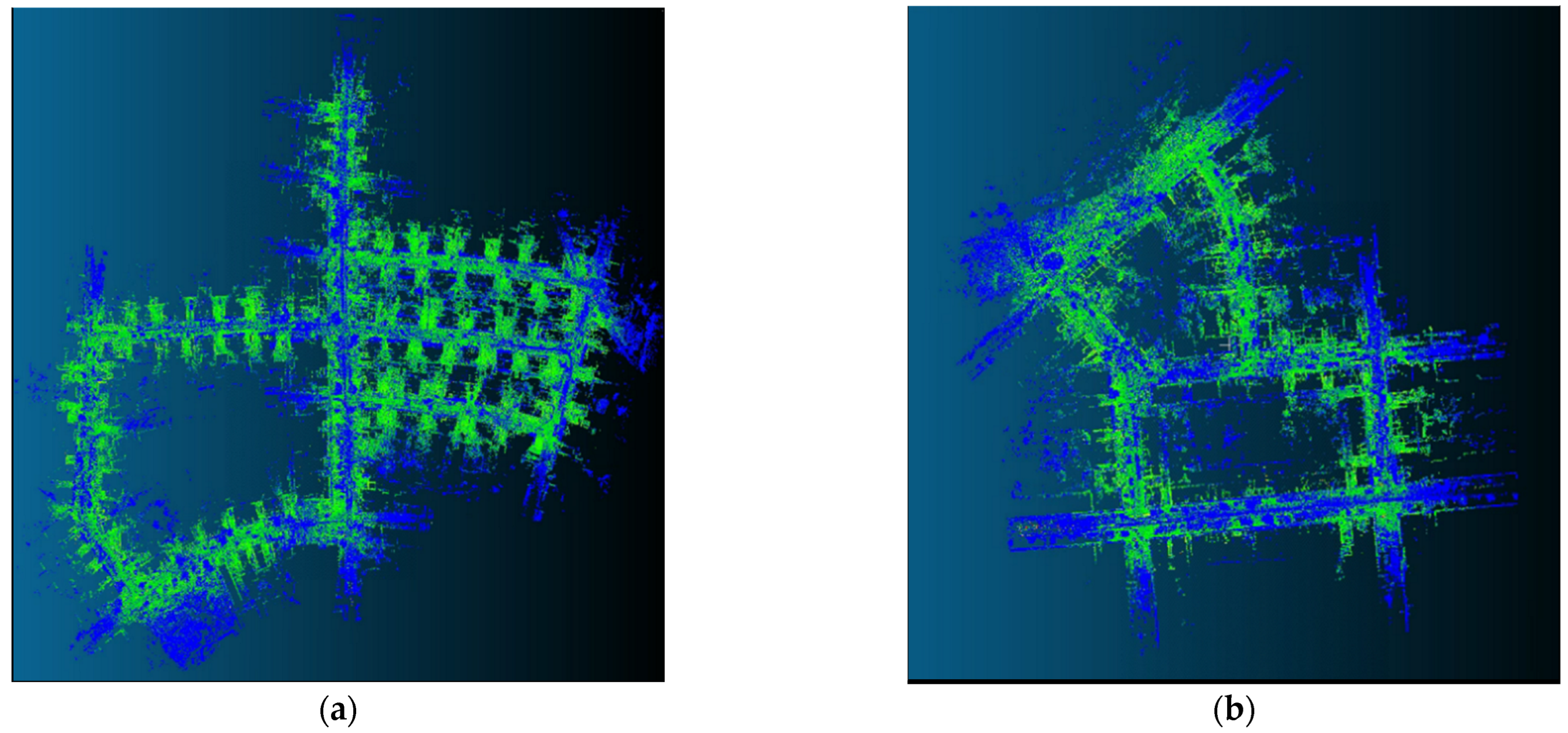The actual mapping effect of sequences 05 and 07 are shown in Figure 13. According to the point cloud images, our map has no obvious ghosting and drift, indicating that the LoNiC algorithm has excellent mapping ability in general scenes. According to the mapping trajectories of sequences 05 and 07 on the KITTI dataset shown in Figure 14, the trajectories estimated by the LoNiC method proposed in this paper are closer to the ground truth compared with LeGO-LOAM. The reason is that LeGO-LOAM just adopts a single distance constraint to identify adjacent frame point cloud data and ignores reliable feature correspondence in complicated environments. Differently, our method employs a multi-scale constraint description to enhance the discrimination of the difference of point cloud data between frames and improve the reliability of feature correspondence. Experimental results suggest that the precision of translation and rotation estimation can be effectively improved by introducing neighborhood information constraints in the SLAM framework.

4.2.2. Experiments on the JLU Dataset

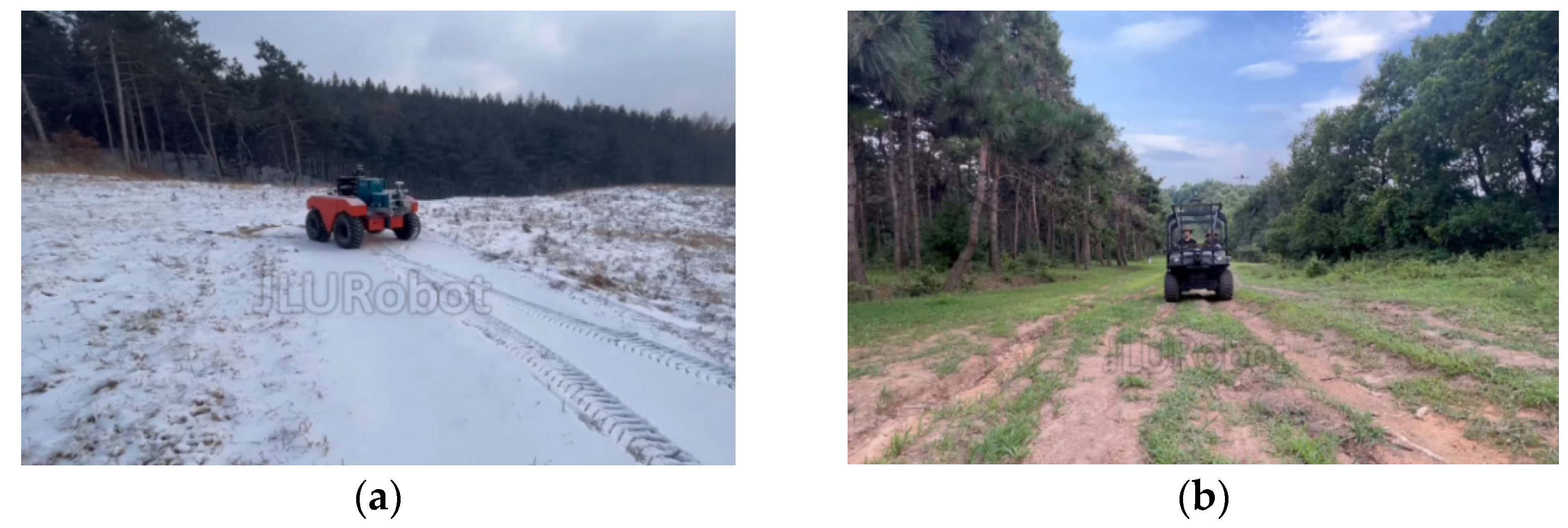
In order to verify the performance of the method proposed in this paper, we collected data from four sections of rugged roads that contained undulating roads on the campus of Jilin University. The mean relative pose error (mRPE), which was used to evaluate the experiment results, was employed on the JLU dataset in the same way that it was on the KITTI dataset.

• Ablation Experiment

First, we contrasted the odometry of LoNiC and LIO-SAM to demonstrate the superior performance of odometry in rugged terrains.

Table 5. Relative pose error of LIO-SAM and LoNiC on the JLU campus dataset.

	Method	LIO-SAM	LoNiC
Sequence
JLU_062801		1.9931/0.0117	2.3454/0.0115
JLU_062802		3.3995/0.0214	2.1599/0.0085
JLU_070101		3.1710/0.0281	2.7353/0.0265
JLU_070102		4.6606/0.0247	4.2571/0.0225
Average		3.3061/0.0215	2.8744/0.0173

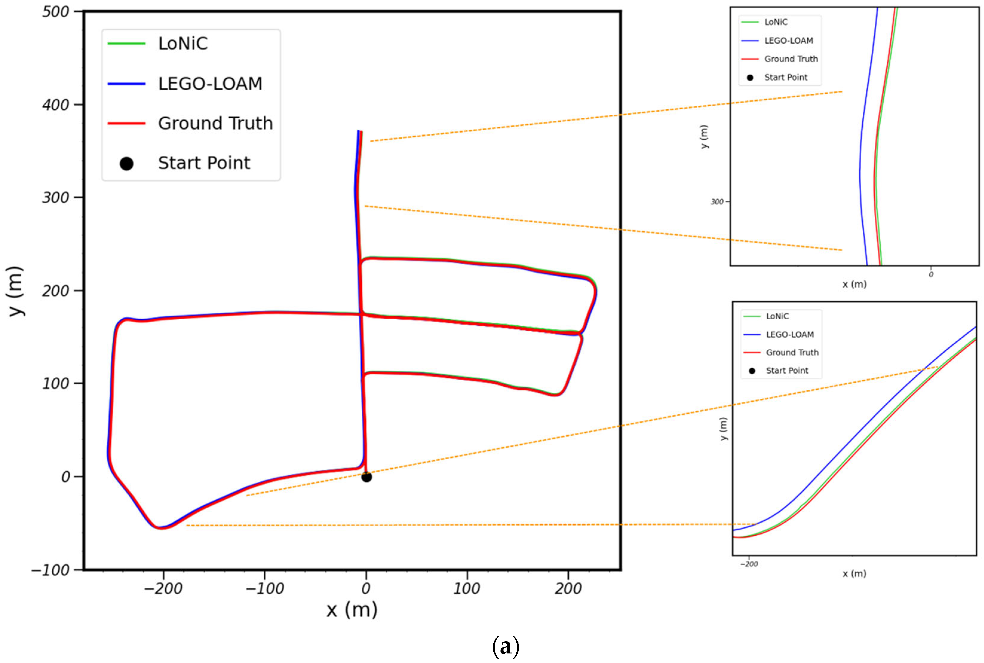
Note: Relative translation error (%)/relative rotation error (°/m). Bold numbers indicate the best performance.

demonstrates that LoNiC performs better than LIO-SAM in most sequences on the JLU campus dataset, with a slightly worse relative rotation error than LIO-SAM on JLU-062801. The mean relative translation error of LoNiC is 3.3061%, which is 0.4317% lower than that of LIO-SAM; the mean relative rotation error of LoNiC is 0.0173°/m, which is 19.53% lower than that of LIO-SAM. This is because the road surface is bumpy in the region of data acquisition, while LIO-SAM is based on the premise of structural roads without consideration of the changes caused by point cloud pitching. Therefore, the odometry based on neighborhood information constraints has stronger discrimination against the difference between feature points of adjacent frames than the traditional odometry based on distance information constraints, thus improving the precision of point cloud registration. As a result, the LoNiC method has more advantages on the JLU campus dataset than the KITTI dataset. According to the trajectory of sequence JLU_070101 on the JLU campus dataset shown in Figure 15, there is no obvious drift of the odometry in both LoNiC and LIO-SAM when the vehicle starts to move. However, the cumulative errors of the LIO-SAM method gradually rise over time and deviate from the ground truth, while the LoNiC method still shows no obvious drift. Based on this, it can be concluded that the LoNiC method proposed in this paper can effectively reduce the cumulative errors of mapping compared with the odometry method based on LIO-SAM, and the figure obtained by the estimated trajectory is the closest to the ground truth.

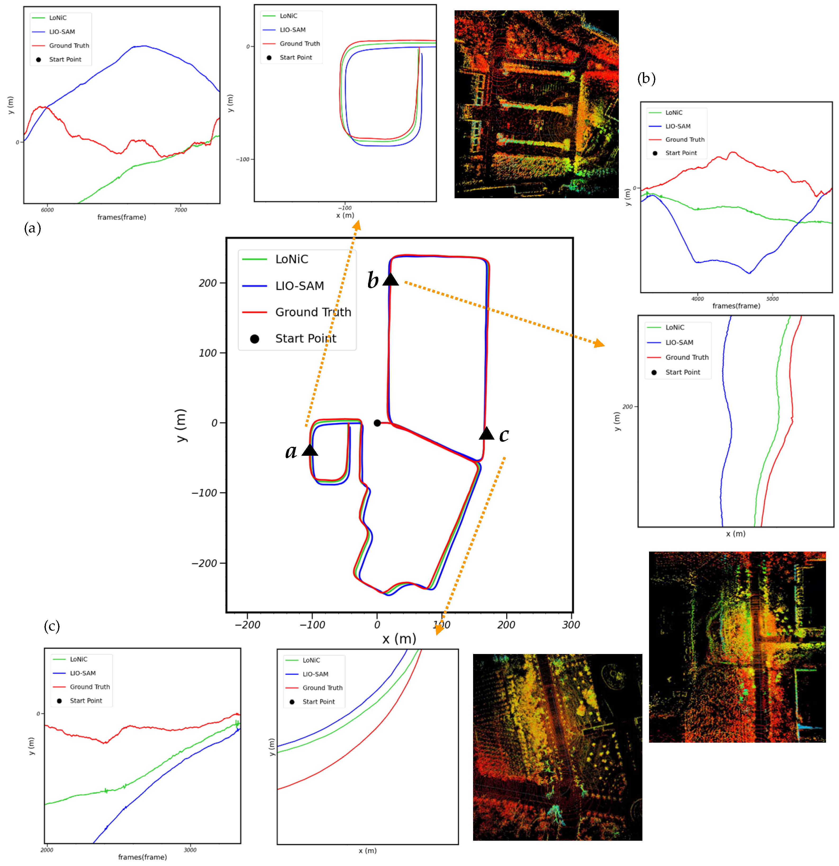
To better prove the performance of LoNiC, three sections of rugged roads in the sequence JLU_070101 were selected for display, and their positions are shown in Figure 15 according to the a, b, and c of the trajectory diagram. Each section is shown in three small figures. The first figure displays the comparison of elevation fluctuation trend of the current road section; the second figure displays the comparison of horizontal mapping trajectories of the current road section; the third figure displays the mapping performance of the current road section. According to Figure 15a, the elevation change trend estimated by the LoNiC algorithm and the LIO-SAM method in the first half section of the data is far from the ground truth. The possible reason is that the first half section of the data is characterized by many trees and no obvious buildings, so it is difficult to extract valuable feature points, particularly in the case of vehicle undulation. However, in the second half of the data, the surface features increase as the vehicle passes through the teaching buildings, and the LoNiC algorithm gradually fits the ground truth, while the elevation estimation of the LIO-SAM method still deviates from the ground truth, indicating an advantage in the feature discrimination of the LoNiC method proposed in this paper. Additionally, as shown in the mapping trajectory, considering that point a is at the end of data acquisition, which is the most significant position of drift for mapping algorithms, the results of the LoNiC method are closer to the ground truth compared with the LIO-SAM method although the LoNiC algorithm has a certain degree of cumulative errors. This suggests that the LoNiC method can ensure the precision of the odometry for a longer time. The road section corresponding to Figure 15b is relatively narrow and long, with buildings on both sides. Theoretically, it is more suitable for the surface feature extraction in the LIO-SAM method. However, the undulation of the data due to the rugged terrains interferes with the corresponding relationship between the feature points, resulting in mis-registration and ultimately leading to large errors in the elevation estimation. The multiple constraints adopted in the LoNiC method can lessen the possibility of mis-registration to a certain extent, thus leading to smaller errors as well as a fluctuation trend that is more similar to the actual situation from the perspective of results. Compared with the first two sections, the road section corresponding to Figure 15c has a wider surrounding environment and fewer reference landmark buildings or objects. Therefore, the performance of the two algorithms is similar to that of the first half of Figure 15a. Although the result of the LoNiC method is close to the ground truth, there is still a gap. In conclusion, the elevation trend and horizontal mapping trajectory of the LIO-SAM method present greater drift in these three sections on the whole, while the results of the LoNiC method are closer to the ground truth. Hence, it can be concluded that feature points with surface information can enhance the scene description, and multi-scale constraint description can effectively reduce the mis-registration of feature points, better correct the errors in elevation and horizontal direction in the case of road fluctuation, and further improve the overall mapping precision.

2.

Comparative Experiment

The LoNiC and LeGO-LOAM methods are compared on the JLU campus dataset in this section to verify the excellent registration precision and mapping effect of the LoNiC method in rugged scenes.

Table 6. Relative pose error of LIO-LOAM and LoNiC on the JLU campus dataset.

	Method	LIO-LOAM	LoNiC
Sequence
JLU_062801		1.7278/0.0100	2.3454/0.0115
JLU_062802		4.1948/0.0269	2.1599/0.0085
JLU_070101		4.3408/0.0282	2.7353/0.0265
JLU_070102		5.7936/0.0268	4.2571/0.0225
Average		4.0143/0.0230	2.8744/0.0173

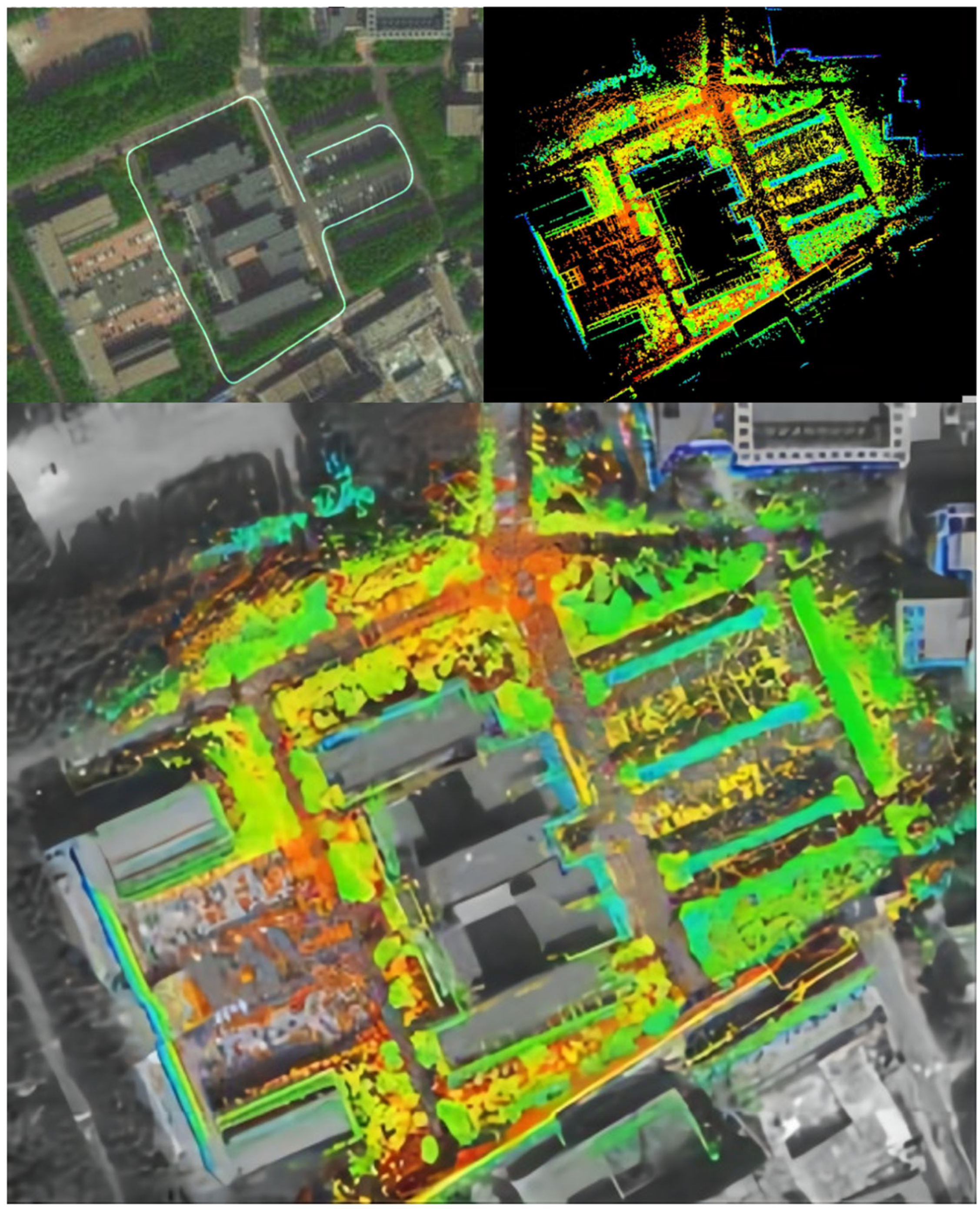
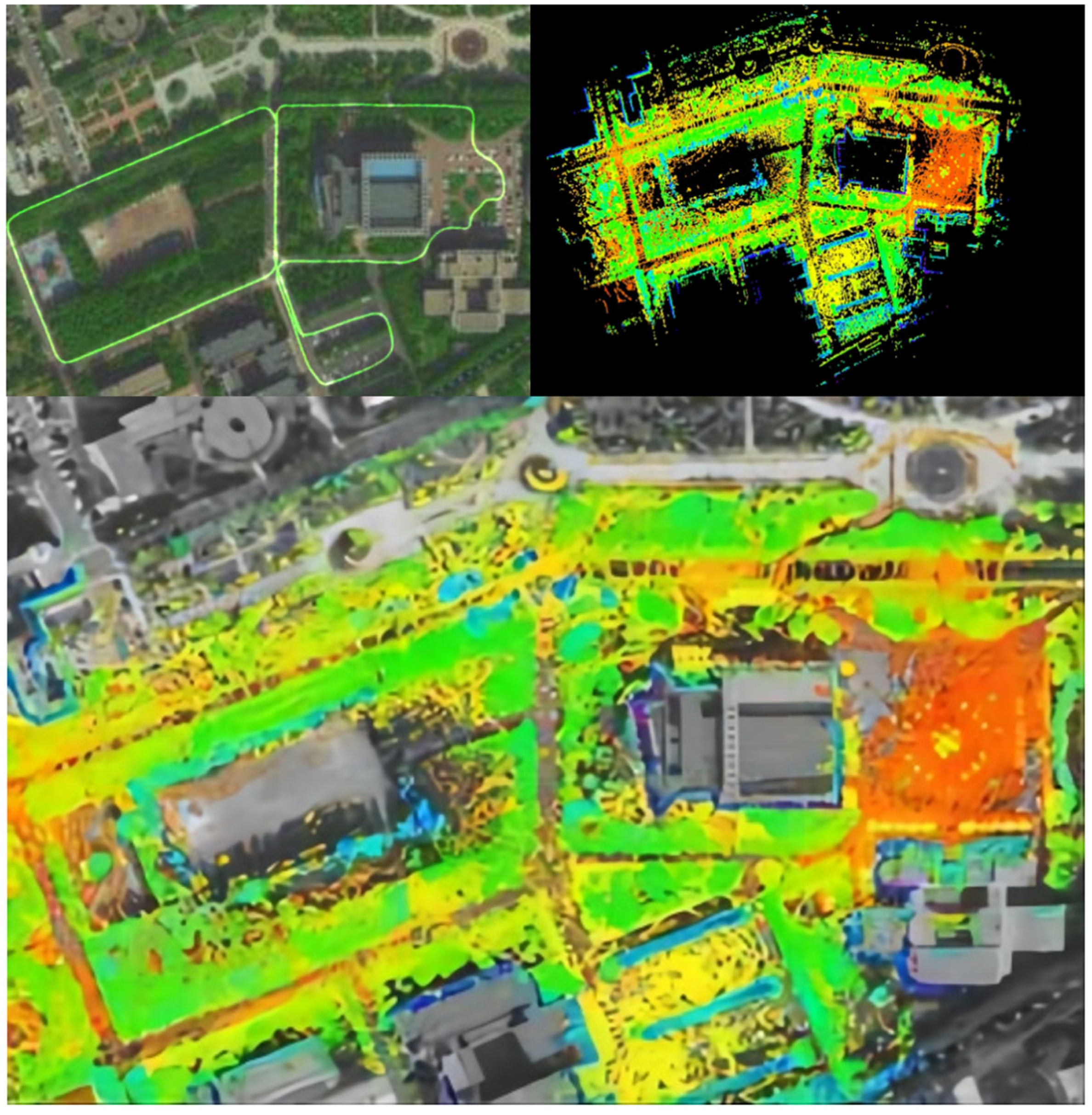
Note: Relative translation error (%)/relative rotation error (°/m). Bold numbers indicate the best performance.

demonstrates that the LoNiC method significantly improved over the LeGO-LOAM method in the mRPE results on the JLU campus dataset, including the sequences of JLU_062802, JLU_070701, and JLU_070702. Specifically, the mean relative translation error of the LoNiC method is 2.8744%, while that of the LeGO-LOAM method is 4.0143%, realizing an improvement of 1.1399%. Similarly, the mean relative rotation error of the LeGO-LOAM method is 0.0230°/m, while that of the LoNiC method is 0.0173°/m, reducing the error by 24.78% compared with LeGO-LOAM. Additionally, the LoNiC method performs much better in the JLU_070701 and JLU_070702 sequences than the LeGO-LOAM method, indicating that the LoNiC method has a greater registration precision for long sequences. The feature points with surface information extracted by LoNiC are more discriminative in complex environments, which effectively improve the accuracy of point cloud registration compared with the corner points and surface points extracted by LeGO-LOAM. With the gradual growth of the motion trajectory, the cumulative error generated by LeGO-LOAM grows quickly compared with that of LoNiC, which indicates that LoNiC outperforms LeGO-LOAM on long sequences. The actual effect of the LoNiC method on the JLU_062801 and JLU_070101 sequences in the JLU campus dataset are displayed in Figure 16 and Figure 17. The following three images are the bird’s-eye view (BEV) image, the point cloud image generated by LoNiC, and the superimposed renderings of the BEV image and the point cloud image. The two superimposed renderings suggest that the point cloud map generated by the proposed LoNiC algorithm can be highly coincident with the actual scenes, whether it is a short-range mapping (≤1 km) or a long-range mapping (≥2 km), which further proves the excellent mapping effect of the LoNiC algorithm.

5. Conclusions

This paper proposed a LiDAR simultaneous localization and mapping (SLAM) algorithm based on neighborhood information constraints for rugged terrains. On the one hand, the pitching of vehicles due to the undulating roads in rugged scenes will decrease the overlapping area of the point clouds of the two adjacent frames, making it impossible to guarantee that the same features can be extracted from the two adjacent frames using an extraction method based on edge and planar points. On the other hand, the current odometry method does not take point cloud pitching into account, so the correspondence between the feature points cannot be guaranteed by relying solely on the distance between the feature points as a constraint, which can result in mis-registration or matching failure. Therefore, this paper utilized the surface feature information for the adaptive extraction of feature points and improved the describing ability in the scene by using the surface characteristics of the point cloud that are unaffected by scene changes. Then, the multi-scale constraint description was used for multiple constraints on feature point matching, precise feature point matching, and the reduction of mis-registration and matching failure in undulating road conditions. On the one hand, ablation experiments demonstrate the effectiveness of our feature extraction method in front-end odometry. Compared with the front-end odometry of LIO-SAM, the mean relative translation error and rotation error of the front-end odometry of our proposed LoNiC on the KITTI dataset is reduced by 0.0782% and 1.04%, and the mean relative translation error and rotation error is reduced by 0.4317% and 19.53% on the JLU dataset, respectively. On the other hand, we conducted comparative experiments on the JLU dataset, and the mean relative translation error is 2.8744% and the average relative rotation error is 0.0173 (°/m). Compared with LEGO-LOAM, the mean relative translation error and rotation error is reduced by 4.0143% and 24.48%, respectively. Meanwhile, the fitting trend in elevation is closer to the ground truth, showing higher mapping accuracy than other advanced methods. The above experiments show that the proposed method has a better processing effect on rugged environments.

In the future work, we will focus on optimizing the feature extraction method and enhancing the feature description by using a machine learning correlation method [28,29] to improve the computational efficiency and testing the proposed algorithm in more scenarios.

References

1. Thrun, S. Probabilistic robotics. Commun. ACM 2002, 45, 52–57. [Google Scholar] [CrossRef]
2. Li, S.; Li, L.; Lee, G.; Zhang, H. A Hybrid Search Algorithm for Swarm Robots Searching in an Unknown Environment. PLoS ONE 2014, 9, e111970. [Google Scholar] [CrossRef] [PubMed]
3. Besl, P.J.; McKay, N.D. Method for registration of 3-D shapes. In Proceedings of the Sensor Fusion IV: Control Paradigms and Data Structures, Boston, MA, USA, 30 April 1992; pp. 586–606. [Google Scholar]
4. Chen, Y.; Medioni, G. Object modelling by registration of multiple range images. Image Vis. Comput. 1992, 10, 145–155. [Google Scholar] [CrossRef]
5. Segal, A.; Haehnel, D.; Thrun, S. Generalized-icp. In Proceedings of the 2009 Robotics: Science and Systems, University of Washington, Seattle, WA, USA, 28 June 28–1 July 2009; p. 435. [Google Scholar]
6. Du, S.; Liu, J.; Zhang, C.; Zhu, J.; Li, K. Probability iterative closest point algorithm for m-D point set registration with noise. Neurocomputing 2015, 157, 187–198. [Google Scholar] [CrossRef]
7. Zhang, J.; Singh, S. LOAM: Lidar Odometry and Mapping in Real-time. In Proceedings of the 2014 Robotics: Science and Systems, Berkeley, CA, USA, 13–15 July 2015; pp. 1–9. [Google Scholar]
8. Shan, T.; Englot, B. Lego-loam: Lightweight and ground-optimized lidar odometry and mapping on variable terrain. In Proceedings of the 2018 IEEE/RSJ International Conference on Intelligent Robots and Systems (IROS), Madrid, Spain, 1–5 October 2018; pp. 4758–4765. [Google Scholar]
9. Hess, W.; Kohler, D.; Rapp, H.; Andor, D. Real-time loop closure in 2D LIDAR SLAM. In Proceedings of the 2016 IEEE international conference on robotics and automation (ICRA), Stockholm, Sweden, 16–21 May 2016; pp. 1271–1278. [Google Scholar]
10. Park, C.; Moghadam, P.; Kim, S.; Elfes, A.; Fookes, C.; Sridharan, S. Elastic lidar fusion: Dense map-centric continuous-time slam. In Proceedings of the 2018 IEEE International Conference on Robotics and Automation (ICRA), Brisbane, QLD, Australia, 21–25 May 2018; pp. 1206–1213. [Google Scholar]
11. Koide, K.; Miura, J.; Menegatti, E. A portable three-dimensional LIDAR-based system for long-term and wide-area people behavior measurement. Int. J. Adv. Robot. Syst. 2019, 16, 1729881419841532. [Google Scholar] [CrossRef]
12. Behley, J.; Stachniss, C. Efficient Surfel-Based SLAM using 3D Laser Range Data in Urban Environments. In Proceedings of the 2018 Robotics: Science and Systems, Pittsburgh, PA, USA, 26–30 June 2018; p. 59. [Google Scholar]
13. Palomer, A.; Ridao, P.; Ribas, D.; Mallios, A.; Gracias, N.; Vallicrosa, G. Bathymetry-based SLAM with difference of normals point-cloud subsampling and probabilistic ICP registration. In Proceedings of the 2013 MTS/IEEE OCEANS-Bergen, Bergen, Norway, 10–14 June 2013; pp. 1–8. [Google Scholar]
14. Trehard, G.; Alsayed, Z.; Pollard, E.; Bradai, B.; Nashashibi, F. Credibilist simultaneous localization and mapping with a lidar. In Proceedings of the 2014 IEEE/RSJ International Conference on Intelligent Robots and Systems, Chicago, IL, USA, 14–18 September 2014; pp. 2699–2706. [Google Scholar]
15. Arth, C.; Pirchheim, C.; Ventura, J.; Schmalstieg, D.; Lepetit, V. Instant Outdoor Localization and SLAM Initialization from 2.5D Maps. IEEE Trans. Vis. Comput. Graph. 2015, 21, 1309–1318. [Google Scholar] [CrossRef] [PubMed]
16. Choudhary, S.; Indelman, V.; Christensen, H.I.; Dellaert, F. Information-based reduced landmark SLAM. In Proceedings of the 2015 IEEE International Conference on Robotics and Automation (ICRA), Seattle, WA, USA, 26–30 May 2015; pp. 4620–4627. [Google Scholar]
17. Biber, P.; Straßer, W. The normal distributions transform: A new approach to laser scan matching. In Proceedings of the Proceedings 2003 IEEE/RSJ International Conference on Intelligent Robots and Systems (IROS 2003)(Cat. No. 03CH37453), Las Vegas, NV, USA, 27–31 October 2003; pp. 2743–2748. [Google Scholar]
18. Takeuchi, E.; Tsubouchi, T. A 3-D scan matching using improved 3-D normal distributions transform for mobile robotic mapping. In Proceedings of the 2006 IEEE/RSJ International Conference on Intelligent Robots and Systems, Beijing, China, 9–15 October 2006; pp. 3068–3073. [Google Scholar]
19. Magnusson, M. The Three-Dimensional Normal-Distributions Transform: An Efficient Representation for Registration, Surface Analysis, and Loop Detection. Ph.D. Dissertation, Örebro Universitet, Orebro, Sweden, 2009. [Google Scholar]
20. Einhorn, E.; Gross, H.-M. Generic NDT mapping in dynamic environments and its application for lifelong SLAM. Robot. Auton. Syst. 2015, 69, 28–39. [Google Scholar] [CrossRef]
21. Das, A.; Waslander, S.L. Scan registration using segmented region growing NDT. Int. J. Robot. Res. 2014, 33, 1645–1663. [Google Scholar] [CrossRef]
22. Ye, H.; Chen, Y.; Liu, M. Tightly coupled 3d lidar inertial odometry and mapping. In Proceedings of the 2019 International Conference on Robotics and Automation (ICRA), Montreal, QC, Canada, 20–24 May 2019; pp. 3144–3150. [Google Scholar]
23. Shan, T.; Englot, B.; Meyers, D.; Wang, W.; Ratti, C.; Rus, D. Lio-sam: Tightly-coupled lidar inertial odometry via smoothing and mapping. In Proceedings of the 2020 IEEE/RSJ International Conference on Intelligent Robots and Systems (IROS), Las Vegas, NV, USA, 24 October 2020–24 January 2021; pp. 5135–5142. [Google Scholar]
24. Wang, H.; Wang, C.; Chen, C.-L.; Xie, L. F-loam: Fast lidar odometry and mapping. In Proceedings of the 2021 IEEE/RSJ International Conference on Intelligent Robots and Systems (IROS), Prague, Czech Republic, 27 September–1 October 2021; pp. 4390–4396. [Google Scholar]
25. Li, L.; Kong, X.; Zhao, X.; Li, W.; Wen, F.; Zhang, H.; Liu, Y. SA-LOAM: Semantic-aided LiDAR SLAM with loop closure. In Proceedings of the 2021 IEEE International Conference on Robotics and Automation (ICRA), Xi’an, China, 30 May–5 June 2021; pp. 7627–7634. [Google Scholar]
26. Chen, S.W.; Nardari, G.V.; Lee, E.S.; Qu, C.; Liu, X.; Romero, R.A.F.; Kumar, V. SLOAM: Semantic lidar odometry and mapping for forest inventory. IEEE Robot. Autom. Lett. 2019, 5, 612–619. [Google Scholar] [CrossRef] [Green Version]
27. Geiger, A.; Lenz, P.; Urtasun, R. Are we ready for autonomous driving? The kitti vision benchmark suite. In Proceedings of the 2012 IEEE conference on computer vision and pattern recognition, Providence, RI, USA, 16–21 June 2012; pp. 3354–3361. [Google Scholar]
28. Chen, X.-w.; Jeong, J.C. Enhanced recursive feature elimination. In Proceedings of the 2007 Sixth International Conference on Machine Learning and Applications, ICMLA 2007, Cincinnati, OH, USA, 13–15 December 2007; pp. 429–435. [Google Scholar]
29. Wang, Y.; Dong, L.; Li, Y.; Zhang, H. Multitask feature learning approach for knowledge graph enhanced recommendations with RippleNet. PLoS ONE 2021, 16, e0251162. [Google Scholar] [CrossRef] [PubMed]
Figure 1. The schematic diagram of SLAM method in unmanned navigation system.
Remotesensing 14 05229 g001
Figure 2. Data collection platforms from JLUROBOT team: (a) J5; (b) Avenger.
Remotesensing 14 05229 g002
Figure 3. Algorithm overview.
Remotesensing 14 05229 g003
Figure 4. Feature described by surface information extraction.
Remotesensing 14 05229 g004
Figure 5. Surface fluctuation of local neighborhood. The red circle represents the current point cloud   p i , and the blue circles represent the k neighbors around   p i : (a) When λ i 1 = λ i 2 = λ i 3 , the surface fluctuates the most; (b) when λ i 1   λ i 2 ,   λ i 1   λ i 3 , the surface is close to a plane.
Remotesensing 14 05229 g005
Figure 6. Smoothness of the region: (a) undulating region; (b) smooth region.
Remotesensing 14 05229 g006
Figure 7. Multi-scale constraint description matching search.
Remotesensing 14 05229 g007
Figure 8. Registration with dynamic iteration factors.
Remotesensing 14 05229 g008
Figure 9. Point cloud iterative matching process: Q   is iterated to position Q with a smaller offset angle and distance from P .
Remotesensing 14 05229 g009
Figure 10. Mobile platform equipped with sensors (Volkswagen Tiguan).
Remotesensing 14 05229 g010
Figure 11. Trajectory comparison of sequence 01 on the KITTI dataset.
Remotesensing 14 05229 g011
Figure 12. Trajectory comparison of sequence 09 on the KITTI dataset.
Remotesensing 14 05229 g012
Figure 13. Mapping trajectory: (a) mapping trajectory of sequence 05 on the KITTI dataset; (b) mapping trajectory of sequence 07 on the KITTI dataset.
Remotesensing 14 05229 g013
Figure 14. Trajectory comparison: (a) trajectory comparison of sequence 05 on the KITTI dataset; (b) trajectory comparison of sequence 07 on the KITTI dataset.
Remotesensing 14 05229 g014aRemotesensing 14 05229 g014b
Figure 15. Trajectory map of sequence JLU_070101 on the JLU campus dataset: a, b and c refer to the comparison of elevation fluctuation trend, mapping trajectory, and mapping effect of road sections at the marked positions of (ac), respectively.
Remotesensing 14 05229 g015
Figure 16. BEV image of the JLU_062801 sequence, LoNiC mapping results, and the superimposed renderings of the BEV image and the point cloud image (the colored trajectory in the BEV image refers to the actual trajectory of the Volkswagen Tiguan).
Remotesensing 14 05229 g016
Figure 17. BEV image of the JLU_070102 sequence, LoNiC mapping results, and the superimposed renderings of the BEV image and the point cloud image (the colored trajectory in the BEV image refers to the actual trajectory of the Volkswagen Tiguan).
Remotesensing 14 05229 g017