Article

A Refined Model for Quad-Polarimetric Reconstruction from Compact Polarimetric Data

1
School of Automation, Northwestern Polytechnical University, Xi’an 710072, China
2
School of Electronic Engineering, Xidian University, Xi’an 710071, China
3
National Key Laboratory of Radar Signal Processing, Xidian University, Xi’an 710071, China
4
Science and Technology on Millimeterwave Laboratory, Beijing Institute of Remote Sensing Equipment, Beijing 100039, China
5
School of Physics and Optoelectronic Engineering, Xidian University, Xi’an 710071, China
*
Author to whom correspondence should be addressed.
Remote Sens. 2022, 14(20), 5226; https://doi.org/10.3390/rs14205226
Submission received: 6 September 2022 / Revised: 15 October 2022 / Accepted: 17 October 2022 / Published: 19 October 2022
(This article belongs to the Special Issue SAR Images Processing and Analysis)

Abstract

:
As a special dual-polarization technique, compact polarimetric (CP) synthetic aperture radar (SAR) has already been widely studied and installed on some spaceborne systems due to its superiority to quad-polarization; moreover, quad-pol information can be explored and reconstructed from the CP SAR data. In this paper, a refined model is proposed to estimate the quad-pol information for the CP mode. This model involves CP decomposition, wherein the polarization degree is introduced as the volume scattering model parameter. Moreover, a power-weighted model for the co-polarized coherence coefficient is proposed to avoid the iterative approach in pseudo-quad-pol information reconstruction. Experiments were implemented on the simulated Gaofen-3 and ALOS-2 data collected over San Francisco. Compared with typical reconstruction models, the proposed refined model shows its superiority in estimating the quad-pol information. Furthermore, terrain classification experiments using a complex-value convolutional neural network (CV-CNN) were performed on AIRSAR Flevoland data to validate the reconstruction effectiveness for classification applications.

Graphical Abstract

1. Introduction

Synthetic aperture radar (SAR) polarimetry is a widely used technique for the derivation of qualitative and quantitative physical information of land [1,2,3,4,5]. Among polarimetric SAR (PolSAR) systems, quad-polarimetric (quad-pol) SAR can obtain complete polarimetric scattering information, and has been successfully applied in terrain classification [6], crop parameter inversion [7], ship detection [8], and so on. However, the available swath width of quad-pol SAR systems is at least halved compared with conventional SAR systems due to the doubled pulse repetition frequency (PRF) for the interleaved transmission of two orthogonal polarizations. To break through the limitation of the quad-pol SAR mode and achieve a lower system complexity, a special dual-polarization mode, known as the compact polarization (CP) mode, is proposed. Furthermore, three types of CP mode are studied: the π / 4 mode, the dual circular polarimetric (DCP) mode, and the hybrid polarimetric (HP) mode [9,10,11]. Due to the advantages over traditional multi-polarization modes, the CP mode has attracted wide attention in recent years. Satellites with a fixed CP mode have been launched, such as the two mini-radio-frequency (mini-RF) radars onboard the Indian Chandrayaan-2-1 moon mission, the American Lunar Reconnaissance Orbiter (LRO) [12,13], the C-band SAR onboard the Indian remote sensing satellite RISAT-1 [14], the L-band SAR onboard the Japanese remote sensing satelite ALOS-2 with experimental mode [15], and the Canadian C-band RADARSAT Mission (RCM) [16], which all adopt HP mode.
To use the CP data, two categories with which to process the CP data are considered. One category is extracting the features from the CP data directly, such as using stokes vectors [12,13] and eigenvalue decomposition [17,18]. Another is to expand the covariance matrix, which means recovering 3 × 3 matrices information from 2 × 2 matrices. This paper mainly focuses on the latter, in that all the information extraction approaches for the quad-pol SAR can be directly employed for the reconstructed data. In 2005, Souyris et al. [9] proposed the primary model to reconstruct a quad-pol covariance matrix using the π / 4 mode. The reconstruction model is based on reflection symmetry assumption, viz., the correlation between the co-polarized term and cross-polarized term equals to zero. Then the relationship between the ratio of the cross-polarized intensity to the co-polarized intensity and the co-polarized coherence coefficient is constructed, and the reconstruction is solved using the iterative method. This model is suitable for the areas dominated by volume scattering, but not for regions dominated by surface or double-bounce scattering. Nord et al. [19] found that Souyris’ model oversimplified the complexity of natural media and introduced a variable parameter N to correct the constructed relationship by Souyris. However, the parameter N depends on the initial reconstruction result, and the relationship may not be fine in some areas, such as the sea surface and sea ice areas [20].
Thereafter, Collins et al. [21] obtained an empirically fitted parameter expression for Nord’s model from the statistical analysis of ocean data. Li et al. [20] proposed an improved N for oil spill detection, which performed better in comparison with Collins’ model. Espeseth et al. [22] proposed two reconstruction methods aiming at sea ice terrain, where a simpler solution based on the polarization degree was used. Kumar et al. [23] assumed that all depolarization energy is contributed by volume scattering, and proposed a way to directly estimate the cross-polarized intensity through polarization entropy. Yin et al. [24,25,26] introduced polarimetric decomposition into the reconstruction process and followed a formalism reconstruction to all CP modes. Yin also proposed a least-squares (LS) estimator to reconstruct the quad-pol information more accurately, but a local minimum was required for each pixel, resulting in more computation cost than the iterative algorithm. Yue et al. [27] proposed a Wishart–Bayesian optimization model to solve the reconstruction estimation. However, the reconstruction effect heavily depends on the prior knowledge obtained by averaging the quad-pol images of the target region, which is difficult to achieve in practical applications. The fully convolutional network (FCN) was used in the reconstruction [28] and Zhang et al. [29] proposed a reconstruction method based on a convolutional neural network (CNN).
Although some new techniques have been applied to the quad-pol information reconstruction from CP data, most improvements are based on Souyris’ model [19,20,21,24,25,26]. In this way, the estimation of the co-polarized coherence coefficient is the core issue. Therefore, a refined estimation model is proposed in the paper, which is based on polarimetric decomposition. The co-polarized coherence coefficient is modeled as a combination of contributions from different scattering mechanisms. Moreover, the polarization degree is employed as a parameter of volume scattering considering the relationship between polarization degree and volume scattering. The sign of co-polarized coherence coefficient is also considered and realized by replacing its real part for its modulus. From the above, the complete reconstruction process was structured and verified on the measured data. In addition, the following contributions and improvements of the work are presented in this article: (1) the estimation of the co-polarized coherence coefficient is improved according to three-component decomposition, so as to avoid the iterative solution in the reconstruction process; (2) the polarization degree is taken as a flexible parameter after analyzing the relationship between the polarization degree and volume scattering model, in order to adapt to different terrain types; (3) considering the sign of the co-polarized coherence coefficient, its modulus is replaced by the real part to retain more information.
The remainder of the paper is organized as follows: In Section 2, the related principle is introduced including three-component decomposition for quad-pol data, and the basic reconstruction model of CP data. Then, the CP decomposition is introduced and a refined method to estimate the co-polarized coherence coefficient is proposed in Section 3, and the entire reconstruction model and process are presented. In Section 4, the experiments on Gaofen-3 and ALOS-2 simulated data are analyzed and discussed, and then the reconstructed AIRSAR Flevoland data is applied to terrain classification using a complex-valued CNN (CV-CNN). Finally, the conclusion is provided in Section 5.

2. Related Basis

2.1. Quad-PolSAR and Freeman-Durden Decomposition

With the H and V linear polarization states, the quad-pol information can be expressed in the form of a scattering matrix, as in Equation (1), which is known as the Sinclair matrix.
  S = [ S H H S H V S V H S V V ]
where S x y denotes the scattering coefficient under transmitted x polarization and received y polarization. Under the backscattering reciprocity assumption, the scattering matrix can be formalized in terms of a scattering vector, as in Equation (2), and the 3 × 3 polarimetric covariance matrix is achieved, as in Equation (3).
k = [ S H H 2 S H V S H V ] T
C = k · k * =   [ | S H H | 2 2 S H H · S H V * S H H · S V V * 2 S H V · S H H * 2 | S H V | 2 2 S H V · S V V * S V V · S H H * 2 S V V · S H V * | S V V | 2 ]
where · denotes the spatial average operation and | · | denotes the modulus. T and * are the matrix transpose and complex conjugation operator, respectively.
To illustrate the scattering characteristics, different polarimetric decompositions were developed. In addition, one classical model-based decomposition is Freeman–Durden decomposition, which decomposes the polarimetric covariance matrix into three parts corresponding to three scattering mechanisms, as in Equation (4), including surface, double-bounce, and volume scattering [30].
C = f s [ C s ] + f d [ C d ] + f v [ C v ]
where f s , f d , and f v represent the scattering coefficient contributed by surface, double-bounce, and volume scattering, respectively. Moreover, the covariance matrices of the three scattering components are as follows:
[ C s ] = [ | β | 2 0 β 0 0 0 β * 0 1 ] [ C d ] = [ | α | 2 0 α 0 0 0 α * 0 1 ] [ C v ] = [ 1 0 1 / 3 0 2 / 3 0 1 / 3 0 1 ]
where α and β refer to the value of S H H · S V V * belonging to double-bounce and surface scattering, respectively. By substituting Equations (3) and (5) into (4), the following equations are obtained:
{ | S H H | 2 = f s · | β | 2 + f d · | α | 2 + f v | S V V | 2 = f s + f d + f v S H H · S V V * = f s · β + f d · α + f v / 3 | S H V | 2 = f v / 3
To solve the above indefinite equations, the sign of ( S H H · S V V * ) was introduced by Zyl et al. [31] to determine whether the surface or double-bounce scattering component is the dominant contribution, where ( · ) indicates the real part of the complex. While ( S H H · S V V * ) > 0 , surface is regarded as the dominant scattering mechanism and α is set as −1. β = 1 is fixed and the double-bounce is decided as the dominant mechanism while ( S H H · S V V * ) < 0 .
As the volume scattering characteristic might be from randomly layered scatter, e.g., randomly oriented long spherical and elliptical scatter, Freeman [32] improved the volume scattering model in Equation (5), which is shown as
C v = [ 1 0 b 0 1 b 0 b * 0 1 ]
where 0 b 1 and b is a real number. For two stable cases, b = 1 / 3 relates to a dipole and b = 1 relates to a sphere [33]. It can be observed that the volume scattering model in Equation (5) is equal to Equation (7) when b = 1 / 3 .

2.2. Compact-PolSAR and the Classical Reconstruction Approach

Considering that HP mode is generally established in CP systems [14,15,16,34], the scattering vector and the 2 × 2 polarimetric covariance matrix for the CP mode are given as follows, by taking the HP mode as example.
k H P = [ S R H S R V ] T = [ S H H i · S H V S H V i · S V V ] T / 2
[ C H P ] = k · k * = [ C 11 C 12 C 21 C 22 ]   = 1 2 [ | S H H | 2 i · S H H · S V V * i · S H H · S V V * | S V V | 2 ] + 1 2 [ | S H V | 2 i · | S H V | 2 i · | S H V | 2 | S H V | 2 ]   + 1 2 [ 2 ( S H H · S H V * ) S H H · S H V * + S V V * · S H V S H H * · S H V + S V V · S H V * 2 ( S V V · S H V * ) ]
where i is the imaginary unit, and ( · ) denotes the imaginary part of a complex. Under the reflection symmetry assumption, S H H · S H V * = S V V · S H V * = 0 , and then the last term in Equation (9) is omitted. From the above, the quad-pol information could be reconstructed by evaluating five parameters from four observations. Souyris et al. [9] introduced an extra model in Equation (10) to help the estimation, which links the ratio between the cross-polarized intensity and the co-polarized intensity to the co-polarized coherence coefficient ρ .
| S H V | 2 | S H H | 2 + | S V V | 2 = 1 | ρ | N
ρ = S H H · S V V * | S H H | 2 · | S V V | 2
In Souyris’ model, the crucial parameter N is stable as N = 4 in Equation (10). In addition, it is extrapolated from the cases where the backscattering wave is either completely polarized or depolarized. In the completely polarized state, | ρ | is close to 1 and | S H V | 2 is quite small compared to the co-polarized component. In the depolarized state, | ρ | is close to zero and Equation (3) degenerates to an identity matrix, viz., | S H H | 2 = | S V V | 2 = 2 | S H V | 2 . Starting from | S H V | 2 = 0 , | S H V | 2 and ρ are iterated to convergence, and finally the stable estimate of | S H V | 2 is obtained. For the special case | ρ | > 1 encountered during the iteration, | S H V | 2 = 0 and | ρ | = 1 are assigned, and then the iteration ends. The pseudo-quad-pol reconstruction result can be achieved, as shown Equation (12), where | S H V | 2 n is the final result after the n-th iteration, and C i j is the element of the CP covariance matrix given in Equation (9).
C q u a d p o l = [ C 11 | S H V | 2 n 0 i · C 12 + | S H V | 2 n 0 2 | S H V | 2 n 0 i · C 12 * + | S H V | 2 n 0 C 22 | S H V | 2 n ]
As N = 4 is suitable for volume-scattering-dominated regions but not for surface or double-bounce-scattering-dominated regions, such as urban areas, Nord et al. [19] proposed a variable expression for N during the iterations with N = | S H H S V V | 2 / | S H V | 2 . The parameters on the right side of the equation depend on the reconstruction results of Souyris’ model.

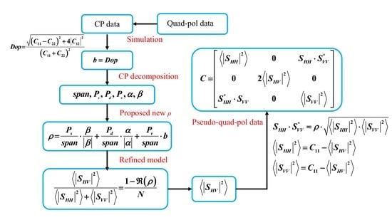
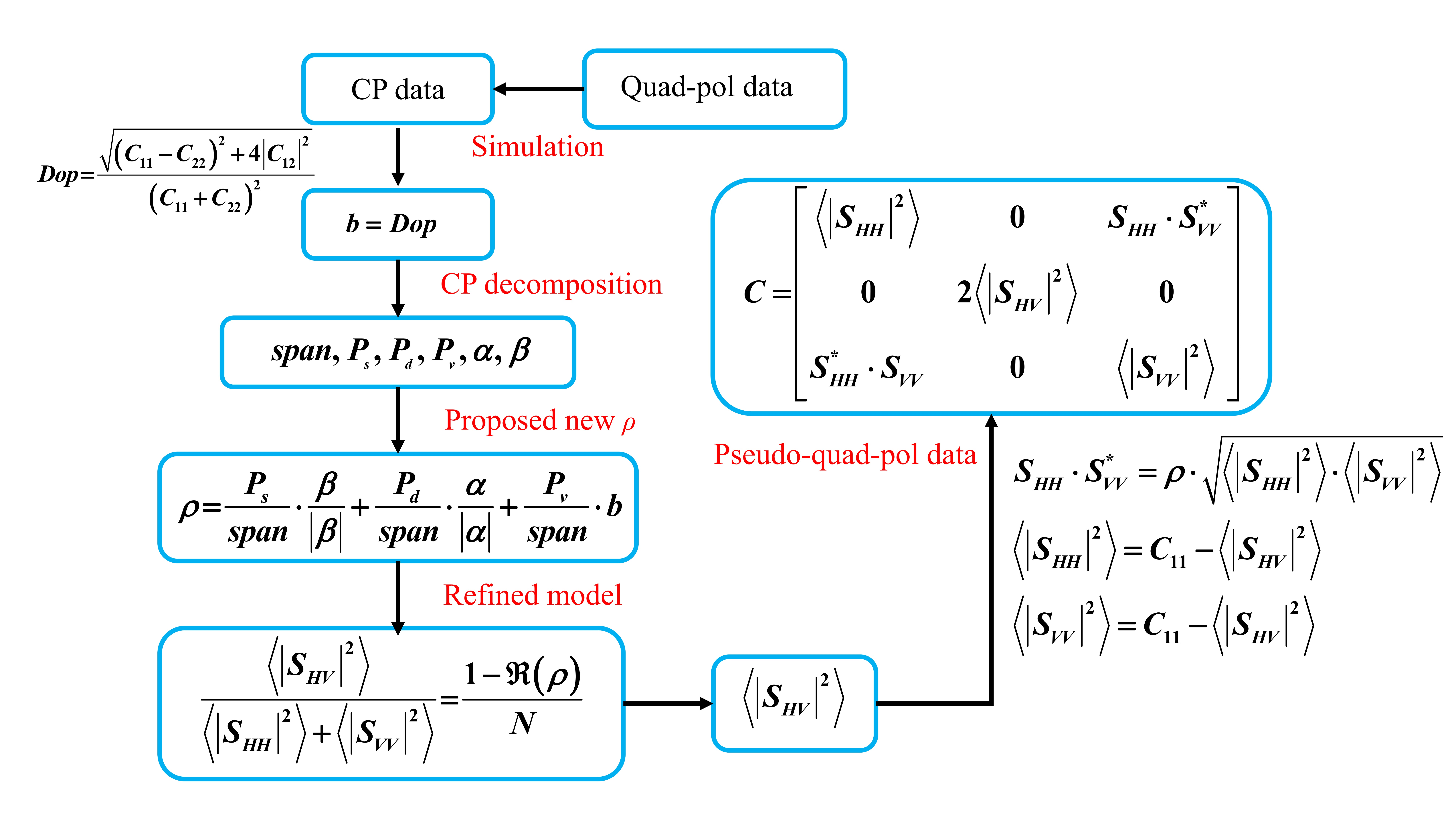
3. Proposed Reconstruction

3.1. CP Decomposition Method

As mentioned in Section 2.1, a flexible parameter b is adopted to improve the Freeman–Durden decomposition for the volume scattering component. The volume scattering matrix degenerates into the unit matrix while b = 0 , which maximizes the freedom degree of backscattering. b is set to be 1/3 in Freeman–Durden decomposition [30] by modeling the volume scattering as completely random dipole scattering. In addition, b = 1 corresponds to model particles as spheres [33]. While increasing the adaptability, the introduction of b also brings difficulties in solving the equations. Freeman settled it by reducing three components to two components, while other researchers used a fixed b [24,25,26,30,35]. However, a fixed b cannot feed different terrain types. Hence, a more flexible parameter should be considered for the parameter b , to satisfy different scattering states.
In Equation (7), 1 b represents the | S H V | 2 component in the model, so b will be quite small while | S H V | 2 is large. The similar relationship exists between | S H V | 2 and the polarization degree [22], which is defined by using the Stokes vector [12] as
D o p = g 1 2 + g 2 2 + g 3 2 g 0
where D o p [ 0 ,   1 ] , and g 0 , g 1 , g 2 , and g 3 are the elements of the Stokes vector. Under the CP mode, Stokes parameters can be obtained from the CP covariance matrix as follows:
[ C C P ] = 1 2 [ g 0 + g 1 g 2 i g 3 g 2 + i g 3 g 0 g 1 ]
In Equation (13), the polarization degree has the same value range as b , which is from 0 to 1. It is known that D o p = 1 implies the completely polarized state and D o p = 0 corresponds to the depolarized state. Between the two limits, the polarized state is regarded as partial polarization. As previously mentioned, b is associated with | S H V | 2 . While b = 1 , viz., 1 b = 0 , | S H V | 2 = 0 is obtained, which corresponds to the completely polarized state. In addition, D o p = 1 describes the same state as above. With the decrease in b , the proportion of | S H V | 2 increases, and the depolarization effect also increases, which corresponds to the decrease in the polarization degree. Finally, when b = 0 , it is obvious that the strongest depolarization effect will be characterized, which corresponds to the case of the lowest polarization degree. Hence, D o p is proposed as a substitution of b in this paper.
After presetting b , the three-component decomposition for CP data by Guo et al. [35] is employed to estimate the three components f s , f d , and f v using the CP mode. Herein, the three 2 × 2 covariance matrices for the three scattering components are formulated as follows:
[ C s ] = [ | β | 2 i · β i · β * 1 ] [ C d ] = [ | α | 2 i · α i · α * 1 ] [ C v ] = [ 3 b 2 ( 3 b 1 ) i 2 ( 1 3 b ) i 2 3 b 2 ]
where b = 1 / 3 in [35], and b = D o p in this paper. Then, the equations in Equation (6) can be deduced to the following:
{ C 11 = f s · | β | 2 + f d · | α | 2 + f v · 3 b 2 C 22 = f s + f d + 3 b 2 · f v C 12 = f s · i β + f d · i α + ( 3 b 1 ) i 2 · f v
Observing Equation (15), it can be seen that the mathematical format of the double-bounce component is the same as the surface component. When the surface scattering model and double-bound scattering model are temporarily combined into one, the volume scattering coefficient can be solved by the following formula:
f v = 1 2 A · ( B 2 4 A · C B ) w h e r e   { A = 2 2 b 2 B = 3 b 2 · ( C 11 + C 22 ) + i C 12 · ( 3 b 1 ) C = | i C 12 | 2 C 11 · C 22
Then, S H H · S V V * can be estimated by S H H S V V * = i C 12 + 1     b 2 · f v . In the remaining model, if R e ( S H H · S V V * ) > 0 , f d is obtained by setting α = 1 , otherwise f s is obtained by setting β = 1 .
{ i f   ( S H H · S V V * ) > 0     t h e n   α = 1 f d = X Y     | Z | 2 X   +   Y   +   2 ( Z ) f s = C 22 f d 3 b 2 · f v β = Z   +   f d f s o r { i f   ( S H H · S V V * ) < 0     t h e n   β = 1 f d = C 22     f s     3 b 2 · f v f s = 2 X Y     | Z | 2 X   +   Y     2 ( Z ) α = Z     f s f d
where X = C 11     3     b 2 · f v , Y = C 22     3     b 2 · f v   , and Z = i C 12     3 b     1 2 f v are residual models after removing volume scattering. In addition, the three scattering power elements are obtained as follows:
{ P s = f s · ( 1 + | β | 2 ) P d = f d · ( 1 + | α | 2 ) P v = f v · ( 3 b )

3.2. Estimation of ρ

The process mentioned in Section 2.2 illustrates that the accuracy of the reconstructed result depends on the estimates of | S H V | 2 and | ρ | . Hence, Yin et al. [24] pointed out that the sign of ρ should be involved during the iteration and rebuilt Equation (10) according to the power of scattering components, including the three components in Equation (4).
Combined with Equation (5), the values of ρ for the three components are achieved as β | β | , α | α | , and b by updating Equation (11). Note that α | α | and β | β | are not always equal to 1 or −1 as arg ( α ) ± π and arg ( β ) 0 . According to three-component decomposition, the covariance matrix can be decomposed into three scattering mechanisms; thus, the coefficient ρ in Equation (11) is regarded as relevant to the three scattering contributions. Then, ρ is redefined as consisting of three parts in Equation (20).
C = f s [ C s ] + f d [ C d ] + f v [ C v ] s p a n · C t r a c e ( C ) = P s · [ C s ] 1   +   | β | 2 + P d · [ C d ] 1   +   | α | 2 + P v · [ C v ] 3     b ρ = f s [ ρ s ] + f d [ ρ d ] + f v [ ρ v ] ρ = P s s p a n · β | β | + P d s p a n · α | α | + P v s p a n · b
where span is the total scattering power. The first formula shows the composition of the covariance matrix in three-component decomposition. P s s p a n , P d s p a n , and P v s p a n are weights of the surface scattering, double-bounce scattering, and volume scattering power in the total scattering power, respectively. Correspondingly, ρ is formalized as a weighted sum of the three scattering components.
Three typical terrain types from Gaofen-3 data were extracted here to verify the performance of the estimate of ρ . Figure 1 illustrates the pseudo-color image of Gaofen-3 data over San Francisco, where three regions: ocean, mountain, and urban areas, were selected and marked. Herein, the ocean area is highlighted with the yellow rectangle, the mountain area is highlighted with red, and the urban area is highlighted with blue. The three test regions are all 400 × 400 pixels in size in the image.
The proposed ρ value in Equation (20) is compared to the real ρ value defined in Equation (11) in Figure 2 and Figure 3. In the figures, the scattering points lie along the diagonal line to support the validity of the polarization state model. Figure 2a–c illustrate the real part of ρ and Figure 3a–c show the imaginary part. The color bar indicates the scatterer number ranging from 0 to 50. It is easy to see that the estimates of ρ in the ocean terrain are quite close to the real ρ value, whose real parts are almost equal to 1 and whose imaginary parts are relatively close to 0, which implies a completely polarized state. In the mountain scene, the real and the imaginary parts of ρ are mainly concentrated in (−0.5, 0.5), and most estimates of the scattering point are close to the real ρ value. The real and the imaginary parts of ρ disperse from −1 to 1 in the urban scene, and the estimation results of ρ are not as good as those for the other scenes. Overall, the estimates of ρ are all around the real values. For quantitative evaluation, the mean errors between the proposed ρ value in Equation (20) and the real ρ value in Equation (11) were calculated and are listed in Table 1. The mean errors for the three tested regions are not far from being less than 0.1. In addition, it can be observed that the estimated ρ value in Equation (20) performs quite well in the ocean scene, but the performance degrades seriously in the urban scene.

3.3. Reconstruction Method

According to the new ρ value proposed in Section 3.2, the stable estimate of ρ can be obtained directly using Equation (20). Therefore, the iterative estimation process mentioned in Section 2.2 can be omitted, which greatly reduces the time cost. Then, the reconstruction of | S H V | 2 is achieved by directly using Equation (10). In addition, the right item in Equation (10) ignores the sign of ρ [25] and directly takes the modulus value. However, the real part of ρ is negative in many cases, such as the illustration in Figure 2c. Hence, Equation (10) is redefined as follows:
| S H V | 2 | S H H | 2 + | S V V | 2 = 1 ( ρ ) N
As shown in Figure 2 and Figure 3, the real part of ρ is always larger than the imaginary part, especially in the ocean area. The statistical mean value of | ( ρ ) | ρ | | is 0.9074 for the data shown in Figure 1, indicating that ( ρ ) guarantees the main information of | ρ | . Moreover, ( ρ ) retains the sign information, so ( ρ ) is used to replace | ρ | in the paper as shown in Equation (21).
As mentioned in Section 2.2, Nord proposed a variable N, so the following Equation (22) can be used to obtain the value of N from the aforementioned CP decomposition.
N = C 11 + C 22 2 ( i C 12 ) 4 1     b 2 · P v 3     b 1     b 2 · P v 3     b
In addition, | S H V | 2 can then be estimated as follows:
| S H V | 2 = C 11 + C 22 2 · 1 ( ρ ) N / 2 + 1 ( ρ )
Finally, the pseudo-quad-pol covariance matrix is reconstructed as shown in Equation (24).
C q u a d p o l = [ C 11 | S H V | 2 0 ρ · ( C 11 | S H V | 2 ) · ( C 22 | S H V | 2 ) 0 2 | S H V | 2 0 ρ * · ( C 11 | S H V | 2 ) · ( C 22 | S H V | 2 ) 0 C 22 | S H V | 2 ]
In summary, the complete process of the proposed reconstruction method is as follows.
Step 1: Data preparation. The 2 × 2 CP covariance matrix is prepared using Equation (9).
Step 2:Polarization degree estimation. The relationship between the polarization degree and CP covariance matrix is given in Equations (13) and (14), and the calculation formula of the polarization degree is then achieved as in Equation (25):
D o p = ( C 11 C 22 ) 2 + 4 | C 12 | 2 ( C 11 + C 22 ) 2 .
Step 3: CP decomposition. Firstly, the parameter b of the volume scattering model in Equation (7) is set as the polarization degree. Then, the CP decomposition is implemented according to Equations (17)–(19). In addition, the decomposition results include the scattering components P s , P d , P v , and the model parameters α , β .
Step 4: Model parameter estimation. The parameter ρ in the quad-pol information reconstruction model is estimated using the CP decomposition results, according to Equation (20). Thus, the iteration procedure employed in Section 2.2 is avoided, and the computational complexity is sharply reduced. Moreover, the parameter N is obtained by using Equation (22).
Step 5: Quad-polarimetric information reconstruction. Cross-polarized intensity | S H V | 2 is firstly reconstructed using Equation (23), and other parameters in the pseudo-quad-polarimetric covariance matrix are then obtained according to Equation (24).

4. Experiments and Discussion

In this section, the experiments implemented using Gaofen-3 data and ALOS-2 data over San Francisco to verify the proposed model are discussed. Moreover, the Flevoland data collected by AIRSAR were employed to further explore the application of the reconstruction result in terrain classification.

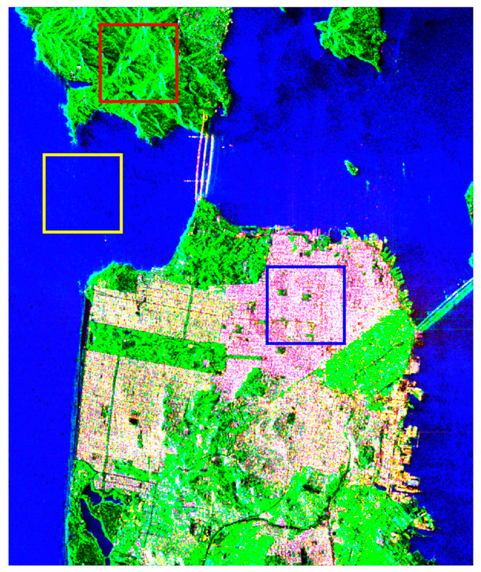
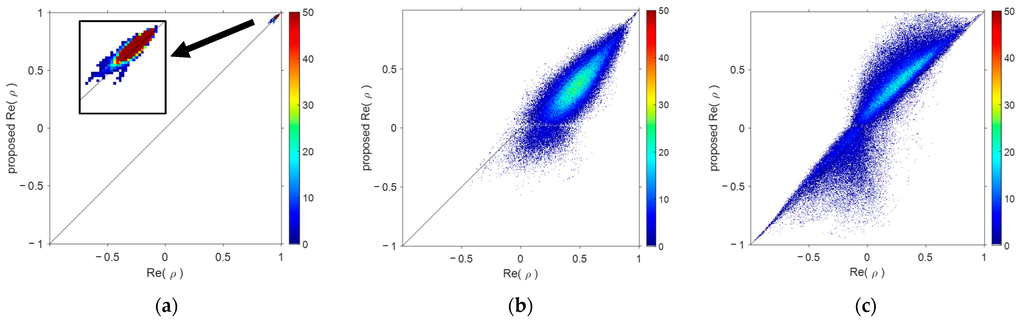
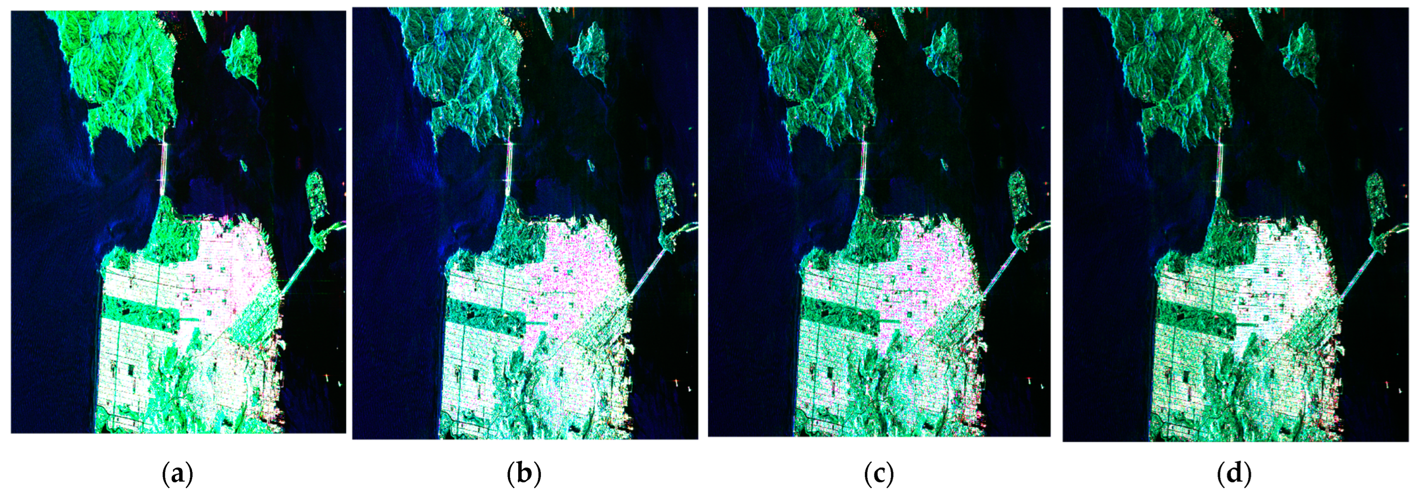
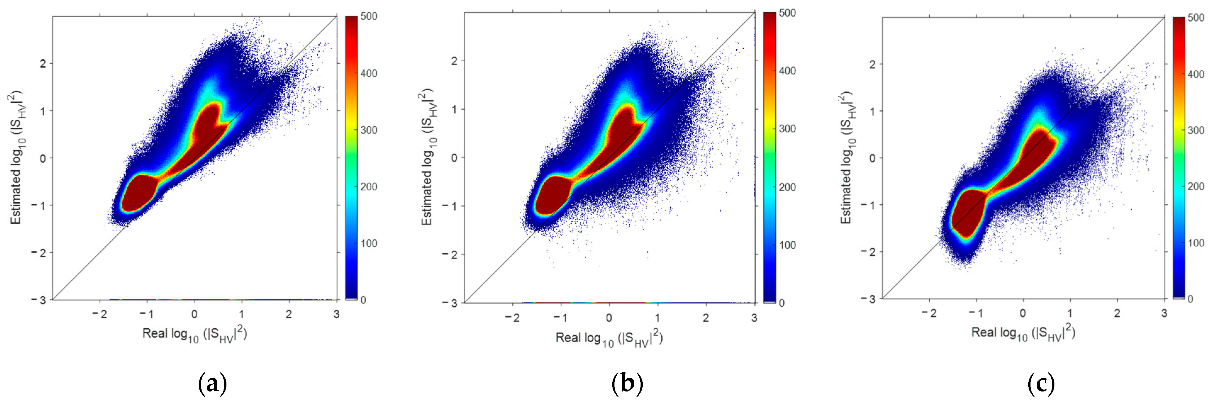
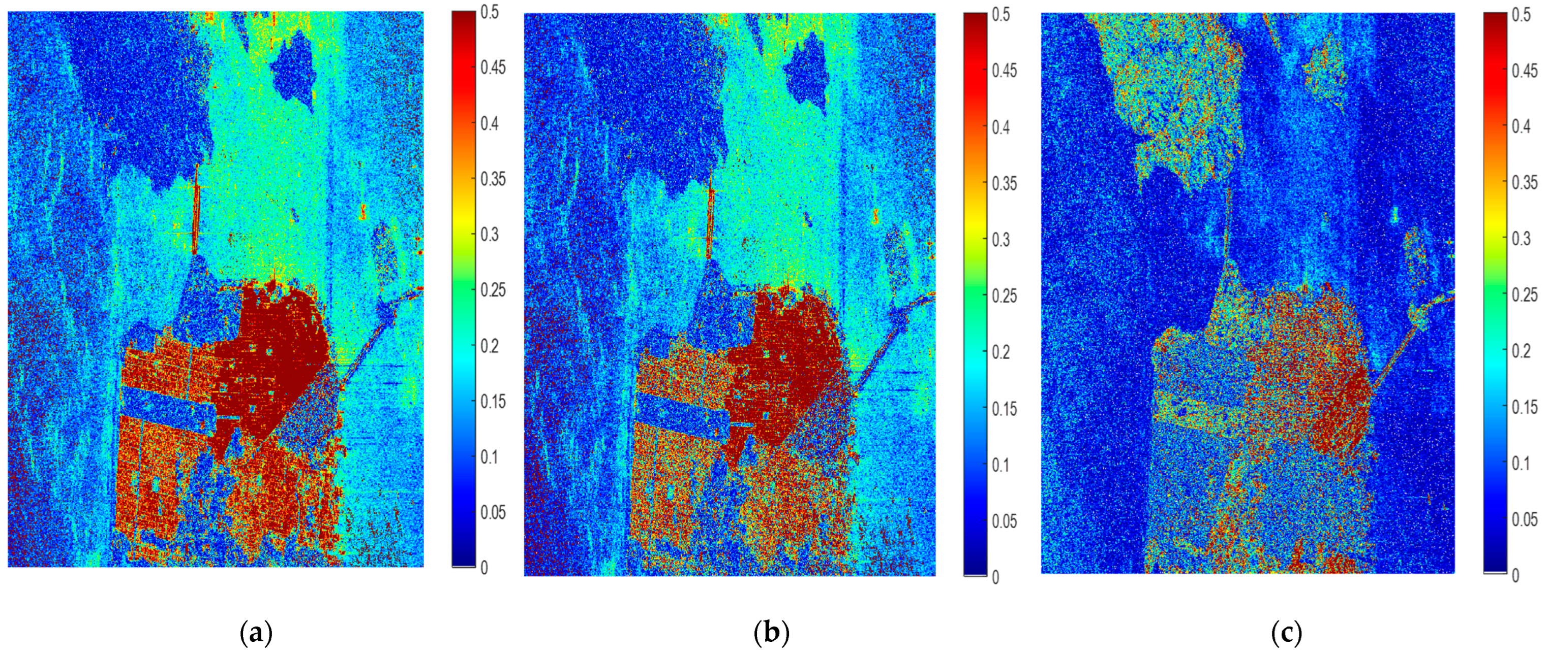
4.1. Experiment on San Francisco Data

4.1.1. Gaofen-3 Data

The experimental dataset was collected by C-band Gaofen-3 with quad-pol mode in 2017. Figure 4a is the pseudo-color image based on the Pauli basis. The size is 3000 × 2500 (range × azimuth) pixels, and the spatial resolution is 5.36 m in azimuth and 2.25 m in range. The CP data were simulated using the quad-pol data according to its specific scattering matrix [19].
The quad-pol reconstruction results with different models are illustrated in Figure 4 in the form of pseudo-color images with Pauli basis. For Souyris’ and Nord’s models, the reconstruction results were finally solved using iterations, as shown in Figure 4b,c. Figure 4d was directly obtained following the procedure described in Section 3.3. It is well established that the urban area in the pseudo-color image with Pauli basis tends to be red, as shown in Figure 4a. However, the performance of the reconstruction models in the urban area was not particularly good due to the complex scattering mechanism of the artificial buildings. In Figure 4b,c, the scattered red color appears in the urban area with quite few texture features. The reason for this is that the parameters exceeded the limits during the iterations and | S H V | 2 was rebuilt to be 0. The absence of green channel led to the appearance of red patches. In Figure 4d, the color of urban area is bright, indicating that | S H V | 2 might be overestimated to some extent.
The evaluation of | S H V | 2 reconstruction result is given in Figure 5 in the form of the comparison between the real value and the reconstructed value, as the performance of | S H V | 2 reconstruction result is of great importance. As more scattering points lying along the diagonal line implies a better reconstruction performance of | S H V | 2 , it is obvious that the proposed method performed best. Souyris’ model significantly overestimated | S H V | 2 due to the empirical value of the model originating from the forest. Nord’s model improved the | S H V | 2 estimates by considering the variable N, but were still a litter inferior to that of Figure 5c. Although the proposed model has several scattering points that deviate significantly owing to it being reconstructed without iteration, there are still more scattering points on both sides of the diagonal, which shows the superiority of the proposed model. It is worth noting that the improvement in the effectiveness of the proposed model is quite apparent when | S H V | 2 is small.
For a better evaluation, the logarithm relative error, as defined in Equation (26), was calculated and is depicted in Figure 6. In Equation (26), | S H V | q u a d 2 and | S H V | C P 2 are the real value and the reconstruction result, respectively. It can be observed that, in Figure 6c, there are more error values close to zero compared to Figure 6a,b, and the reconstruction performance is enhanced in both the ocean region and the urban region. In particular, although the absolute error in urban area is still larger than in other areas, the error in the urban area is significantly reduced in terms of vision. The | S H V | 2 in the urban area is universally smaller, which validates the same conclusion as in Figure 5.
e r r o r l o g = | ( l o g 10 ( | S H V | q u a d 2 ) ) ( l o g 10 ( | S H V | C P 2 ) ) ( l o g 10 ( | S H V | q u a d 2 ) ) |
In order to quantitatively analyze the reconstruction results, statistical metrics, such as the reconstruction error and the cross-entropy, were employed. The reconstruction error is given by | ( X q u a d X C P ) / X q u a d | , where X q u a d is the original value of quad-pol data, and X C P is the value of the reconstruction data. The mean value measures the bias in the reconstruction result with respect to the quad-pol data, and the standard deviation (Std.) measures the error deviation level referring to the mean error. Mean and Std. can evaluate the reconstruction accuracy from a statistical perspective, and both decrease as the reconstruction accuracy increases. The mathematical equations for Mean and Std. are shown in Equation (27).
M e a n = 1 K i = 1 K | e r r o r ( i ) | , S t d . = 1 K 1 i = 1 K | e r r o r ( i ) M e a n | 2
where K is the total number of pixels. The cross-entropy (CE) measures the performance by comparing the possibility distribution function (PDF) consistency between the reconstruction results and the original quad-pol data, and decreases as the reconstruction accuracy increases. The definition of CE is given in Equation (28).
CE ( X Y ) = x X , y Y p ( x ) log p ( y ) p ( x )
where p ( x ) and p ( y ) are the PDFs of the original quad-pol data and the reconstruction data. Except for Souyris’ and Nord’s models, the methods proposed by Espeseth [22] and Kumar [23] were also taken for comparison and discussion. Table 2 compares the proposed model with the aforementioned reconstruction models in detail. In the table, four parameters are used: | S H H | 2 , | S V V | 2 , | S H V | 2 , and | ρ | . Since Espeseth’s model and Kumar’s model do not follow pixel-by-pixel reconstruction, both the time cost and | ρ | were not considered.
As shown in Table 2, the proposed model obtained the minimum mean error on | S H H | 2 , | S V V | 2 , and | S H V | 2 . This indicates that the proposed model is of the highest accuracy. Moreover, the proposed model also achieved good Std. evaluations. In particular, the Mean and Std. of | S H V | 2 were 0.6805 and 1.0342, respectively, using the proposed model, which were significant improvements when compared to the values of 2.2379 and 2.6883 obtained using Souyris’ model. As | S H V | 2 is the core and essential parameter in reconstruction, this enhancement is of great importance. For the metric of CE, the proposed model achieved the best results on almost all parameters compared to other models. The CE of the proposed model for | S H V | 2 was 1/4 of Souyris’ model; furthermore, the CE of the proposed model for | ρ | was 1/8 of Souyris’ model.
While the proposed model achieved the best reconstruction effect, the time cost was also explored and is illustrated in Table 2. The experiments were performed on a PC with 3.0 GHz CPU and 16 GB memory. The time costs show that the proposed method saved more than 400 s in an identical running environment, which is a 20% saving as compared to Souyris’ model.

4.1.2. ALOS-2 Data

The L-band ALOS-2 data over San Francisco collected in 2015 were also employed in the experiment, as shown in the pseudo-color image based on Pauli basis in Figure 7a, which has a size of 5000 × 4000 (azimuth × range) pixels. The spatial resolution is 6 m in azimuth and 4.3 m in range. The CP data were simulated.
The quad-pol reconstruction results with different models are depicted in Figure 7 in the form of pseudo-color images. Figure 7b–d are the results of Souyris’ model, Nord’s model, and the proposed model, respectively. Generally, speckle-like scatterers are apparent in Figure 7b,c in the urban region, and Figure 7d shows better reconstruction result in terms of vision. The comparison between the real value and the reconstructed | S H V | 2 is given in Figure 8 to assess the reconstruction performance. In Figure 8a, most values of | S H V | 2 are overestimated. Compared to Figure 8a, the improvement of Nord’s model seems quite inapparent. By using the proposed model, the estimation was improved while | S H V | 2 was small; and when | S H V | 2 was large, the reconstructed | S H V | 2 was underestimated. Overall, the proposed model caused the most scattering points to fall near to the diagonal on both sides.
For further assessment, the logarithm relative error is depicted as Figure 9. The proposed model had a better effect on the overall scene. Obviously, the error value is closer to zero in Figure 9c. The reconstruction performance of the proposed model in both the ocean region and the urban region improved as compared to Figure 9a,b, and in urban areas in particular, the improvement was greater, which is consistent with the results of the Gaofen-3 data.
Table 3 illustrates the quantitative comparison results using different models. The proposed model performed best on most parameters. Similar to the results of the Gaofen-3 data, the most significant improvement of the proposed model was in the estimation of | S H V | 2 . Comparing the reconstructed | S H V | 2 using the proposed model with Souyris’ model, the mean error and standard deviation reduced from 2.1401 and 3.7699 to 0.5551 and 1.0260, and the cross-entropy reduced from 0.6546 to 0.0638. In addition, the time cost reduced by nearly 23% compared with Souyris’ model. In general, the proposed model was able to greatly improve the reconstruction results.

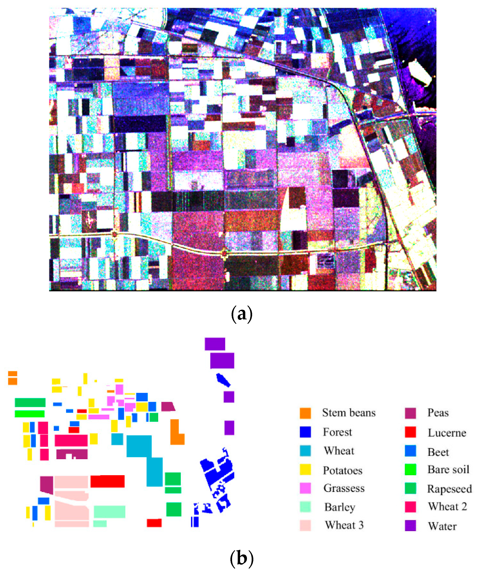
4.2. Experiment on Flevoland Data

4.2.1. Data Set and Reconstruction

In this section, the L-band AIRSAR data acquired over Flevoland are introduced. They were employed for terrain classification to verify the effectiveness of the reconstructed pseudo-quad-pol information using the simulated CP data. Figure 10a is the pseudo-color image decomposed by Pauli decomposition of the quad-pol data, with a size of 1024 × 750 pixels. The ground truth is illustrated in Figure 10b for the following terrain classification. In this area, there are 14 identified terrain types, including stem beans, peas, forest, lucerne, three types wheat, beet, potatoes, bare soil, grass, rapeseed, barley, and water.
With the simulated CP data, the quad-pol reconstruction results were achieved. Figure 11a–c show the pseudo-color images from the reconstructed quad-pol information according to Souyris’ model, Nord’s model, and the proposed model, respectively. The relative error between the real value and the reconstructed | S H V | 2 is shown in Figure 12. It was found that the error in vision was significantly reduced by the proposed model compared to Souyris’ and Nord’s results.

4.2.2. Performance on CV-CNN Classifier

For further analysis of the reconstruction models, the quad-pol data, simulated CP data, and reconstructed data were applied in terrain classification with the deep learning technique, which performs much better than conventional classification algorithms. Here, the CNN was considered and developed for the SAR complex data. Instead of the traditional CNN for real values, the complex convolution network (Complex-Valued-CNN, CV-CNN) proposed by Xu Feng et al. [36] was adopted, which extends the CNN to complex domain for SAR images with phase information, as the coherent phase between polarization channels has important information.
The convolution network employed in this paper includes two convolution layers: one pool layer and one full connection layer, as in [36]. The experimental data were sampled from the 8 × 8 window of the ground truth and extended to the size of 12 × 12 after filling zero. Only data with less than 20 unlabeled pixels in the window were sampled. A fivefold cross-validation [37] approach was carried out in the experiment. All sampling data were randomly divided into five groups, which were used as test sets in turn. In the experiment, the channel number for quad-pol data was six with all normalization parameters of the covariance matrix. For the CP data, three channels were used and the reconstructed data had four channels, as shown in Equations (12) and (24). Moreover, the learning rate was set to be 0.8 and 65 epochs were carried.
The classification results in Figure 13a–e were obtained by the quad-pol data, CP data, and pseudo-quad-pol data reconstructed with Souyris’ model, Nord’s model, and the proposed model, respectively. The figures are all from the same group of the cross-validation experiment. The classification results are listed in Table 4 in terms of the classification accuracy on the test sets. Compared with CP mode and Souyris’ and Nord’s models, the proposed model achieved the highest average accuracy. In particular, the proposed method achieved the best results in the classification of a variety of crops. This shows that the classification accuracy of the pseudo-quad-pol data reconstructed from the proposed model was better than that of the CP data, which verifies the effectiveness of the proposed model. This strongly shows the significance of the reconstruction method and the improvement in the reconstruction accuracy by the proposed model. Although the total accuracy of the reconstructed quad-pol data was not as good as the real quad-pol data, the proposed model performed much better than Souyris’ model, which implies that the proposed model can supply more accurate reconstructed quad-pol information.

4.3. Discussion

From experiments on the Gaofen-3 and ALOS-2 datasets, the proposed model was compared with other models in terms of figure vision and quantitative assessments. The results show the advantages of the proposed model. The comparison of different models is given in Table 5. As the first proposed reconstruction model, Souyris’ model opened the door to the CP reconstruction method. Souyris’ model performed well in the vegetation area, but it did not produce good results in other areas. According to the verification of empirical data, Nord optimized the effect of the model to a certain extent through introducing the parameter N into the model. Espeseth’s model and Kumar’s model, which are less complex, exhibited similar performance to Souyris’ model. In the paper, a refined model based on three-component decomposition is proposed. A new way to estimate ρ through polarimetric decomposition is proposed, and the relationship between | S H V | 2 and ρ is modified. The experiments validated that the precision of the proposed model is higher than that of the other models, and the solution is faster than that of pixel-by-pixel models.

5. Conclusions

In this paper, quad-pol information reconstruction is analyzed and a refined model based on three-component decomposition is proposed. The main concept is to use the estimation of ρ through polarimetric decomposition instead of iteration. Considering different terrain types, the polarization degree is introduced into the model to substitute the volume scattering model parameter. Moreover, ( ρ ) replaces | ρ | in order to retain symbol information. With all the above improvements, the proposed model can realize effective quad-pol information reconstruction from CP data with less computation cost, thus avoiding the iteration process.
Tests using Gaofen-3 data confirmed that the proposed method can estimate ρ relatively well, which lays the foundation for the improvement of the reconstruction results. Moreover, experiments were performed on the San Francisco datasets from both Gaofen-3 and ALOS-2, which validated the superiority of the proposed model in quad-pol information reconstruction as compared to typical models. In particular, the proposed method is far better than the other two methods in estimating | S H V | 2 . Moreover, CV-CNN classification was implemented on AIRSAR Flevoland data for further analysis, showing the effectiveness of the reconstruction model in terrain classification.

Author Contributions

Conceptualization R.G.; Methodology R.G. and X.Z.; Validation and analyzed X.Z.; Writing R.G. and X.Z.; Resources B.Z. and Y.L.; Data preparation J.B. and L.G. All authors have read and agreed to the published version of the manuscript.

Funding

This work was funded by State Key Laboratory of Geo-Information Engineering under grant SKLGIE2020-M-4-2, by Shanghai Aerospace Science and Technology Fund under grant SAST2020-028, and by the National Natural Science Foundation of China (61971326).

Conflicts of Interest

The authors declare no conflict of interest.

References

  1. Moreira, A.; Prats-Iraola, P.; Younis, M.; Hajnsek, I.; Papathanassiou, K.P. A tutorial on synthetic aperture radar. IEEE Geosci. Remote Sens. 2013, 1, 6–43. [Google Scholar] [CrossRef] [Green Version]
  2. Zhou, L.; Yu, H.; Lan, Y.; Gong, S.; Xing, M. CANet: An unsuperivised deep convolutional neural network for efficient cluster-anlysis-based multibaseline InSAR phase unwrapping. IEEE Trans. Geosci. Remote Sens. 2021, 60, 1–15. [Google Scholar] [CrossRef]
  3. Yiğit, E.; Demirci, Ş.; Özdemir, C. Clutter removal in millimeter wave GB-SAR images using OTSU’s thresholding method. Int. J. Eng. Geosci. 2022, 7, 43–48. [Google Scholar] [CrossRef]
  4. Demirci, Ş.; Özdemir, C. An investigation of the performances of polarimetric target decompositions using GB-SAR imaging. Int. J. Eng. Geosci. 2021, 6, 9–19. [Google Scholar] [CrossRef]
  5. Duysak, H.; Yiğit, E. Investigation of the performance of different wavelet-based fusions of SAR and optical images using Sentinel-1 and Sentinel-2 datasets. Int. J. Eng. Geosci. 2022, 7, 81–90. [Google Scholar] [CrossRef]
  6. Ohki, M.; Shimada, M. Large-area land use and land cover classification with quad, compact, and dual polarization SAR data by PALSAR-2. IEEE Trans. Geosci. Remote Sens. 2018, 56, 5550–5557. [Google Scholar] [CrossRef]
  7. Zhang, L.; Meng, M.; Zeng, J.; Wei, X.; Shi, H. Evaluation of Gaofen-3 C-Band SAR for soil moisture retrieval using different polarimetric decomposition models. IEEE J. Sel. Top. Appl. Earth Obs. Remote Sens. 2021, 14, 5707–5719. [Google Scholar] [CrossRef]
  8. Chang, Y.; Anagaw, A.; Chang, L.; Wang, Y.; Hsiao, C.; Lee, W. Ship Detection Based on YOLOv2 for SAR imagery. Remote Sens. 2019, 11, 786. [Google Scholar] [CrossRef] [Green Version]
  9. Souyris, J.; Imbo, P.; Fjortoft, R.; Mingot, S.; Lee, J.-S. Compact polarimetry based on symmetry properties of geophysical media: The π/4 model. IEEE Trans. Geosci. Remote Sens. 2005, 43, 634–646. [Google Scholar] [CrossRef]
  10. Stacy, N.; Preiss, M. Compact polarimetric analysis of X-band SAR data. In Proceedings of the 6th European Conference on Synthetic Aperture Radar, Dresden, Germany, 16–18 May 2006. [Google Scholar]
  11. Raney, R.K. Hybrid-Polarity SAR architecture. IEEE Trans. Geosci. Remote Sens. 2007, 45, 3397–3404. [Google Scholar] [CrossRef]
  12. Raney, R.K.; Cahill, J.T.; Patterson, C.W.; Bussey, D.B. The m-chi decomposition of hybrid dual-polarimetric radar data with application to lunar craters. J. Geophys. Res. Planets 2012, 117, E00H21. [Google Scholar] [CrossRef]
  13. Raney, R.K.; Spudis, P.D.; Bussey, D.B.; Crusan, J.; Jensen, J.R.; Marinelli, W. The lunar mini-RF radars: Hybrid polarimetric architecture and initial results. Proc. IEEE 2011, 99, 808–823. [Google Scholar] [CrossRef]
  14. Turkar, V.; De, S.; Rao, Y.S.; Shitole, S.; Bhattacharya, A.; Das, A. Comparative analysis of classification accuracy for RISAT-1 compact polarimetric data for various land-covers. In Proceedings of the 2013 IEEE International Geoscience and Remote Sensing Symposium-IGARSS, IGARSS 2013, Melbourne, Australia, 21–26 July 2013. [Google Scholar]
  15. Rosenqvist, A.; Shimada, M.; Suzuki, S.; Ohgushi, F.; Tadono, T.; Watanaba, M. Operational performance of the ALOS global systematic acquisition strategy and observation plans for ALOS-2 PALSAR-2. Remote Sens. Environ. 2014, 155, 3–12. [Google Scholar] [CrossRef]
  16. Geldsetzer, T.; Khurshid, S.K.; Warner, K.; Botelho, F.; Flett, D. Wind speed retrieval from simulated RADARSAT Constellation Mission compact polarimetry SAR data for marine application. Remote Sens. 2019, 11, 1682. [Google Scholar] [CrossRef] [Green Version]
  17. Cloude, S.R.; Goodenough, D.G.; Chen, H. Compact decomposition theory. IEEE Geosci. Remote Sens. Lett. 2012, 9, 28–32. [Google Scholar] [CrossRef]
  18. Guo, R.; Liu, Y.-B.; Wu, Y.-H.; Zhang, S.-X.; Xing, M.-D.; He, W. Applying H/α decomposition to compact polarimetric SAR. IET Radar Sonar Navig. 2012, 6, 61–70. [Google Scholar] [CrossRef]
  19. Nord, M.; Ainsworth, T.; Lee, J.-S.; Stacy, N. Comparison of compact polarimetric synthetic aperture radar modes. IEEE Trans. Geosci. Remote Sens. 2009, 47, 174–188. [Google Scholar] [CrossRef]
  20. Li, Y.; Zhang, Y.-Z.; Chen, J.; Zhang, H.-S. Improved compact polarimetric SAR quad-pol reconstruction algorithm for oil spill detection. IEEE Geosci. Remote Sens. Lett. 2014, 11, 1139–1142. [Google Scholar] [CrossRef]
  21. Collins, M.; Denbina, M.; Atteia, G. On the reconstruction of quad-pol SAR data from compact polarimetry data for ocean target detection. IEEE Trans. Geosci. Remote Sens. 2013, 51, 591–600. [Google Scholar] [CrossRef]
  22. Espeseth, M.; Brekke, C.; Anfinsen, S. Hybrid-Polarity and reconstruction methods for sea ice with L- and C-band SAR. IEEE Geosci. Remote Sens. Lett. 2016, 13, 467–471. [Google Scholar] [CrossRef]
  23. Kumar, A.; Panigrahi, R.K. Entropy based reconstruction technique for analysis of hybrid-polarimetric SAR data. IET Radar Sonar Navig. 2019, 13, 620–626. [Google Scholar] [CrossRef]
  24. Yang, J.; Yin, J.; Moon, W. Model-based pseudo-quad-pol reconstruction from compact polarimetry and its application to oil-spill observation. J. Sens. 2015, 2015, 734848. [Google Scholar]
  25. Yin, J.; Papathanassiou, K.; Yang, J.; Chen, P. Least-squares estimation for pseudo quad-pol image reconstruction from linear compact polarimetric SAR. IEEE J. Sel. Top. Appl. Earth Obs. Remote Sens. 2019, 12, 3746–3758. [Google Scholar] [CrossRef]
  26. Yin, J.; Yang, J. Framework for Reconstruction of pseudo quad polarimetric imagery from general compact polarimetry. Remote Sens. 2021, 13, 530. [Google Scholar] [CrossRef]
  27. Yue, D.-X.; Xu, F.; Jin, Y.-Q. Wishart–Bayesian reconstruction of quad-pol from compact-pol SAR image. IEEE Geosci. Remote Sens. Lett. 2017, 14, 1623–1627. [Google Scholar] [CrossRef]
  28. Gu, F.; Zhang, H.; Wang, C. Quad-pol reconstruction from compact polarimetry using a fully convolutional network. Remote Sens. Lett. 2020, 11, 397–406. [Google Scholar] [CrossRef]
  29. Zhang, F.; Cao, Z.; Xiang, D.; Hu, C.; Ma, F.; Yin, Q.; Zhou, Y.S. Pseudo quad-pol simulation from compact polarimetric SAR data via a complex-valued dual-branch convolutional neural network. IEEE J. Sel. Top. Appl. Earth Obs. Remote Sens. 2021, 15, 901–918. [Google Scholar] [CrossRef]
  30. Freeman, A.; Durden, S. A three-component scattering model for polarimetric SAR data. IEEE Trans Geosci. Remote Sens. 1998, 36, 963–973. [Google Scholar] [CrossRef] [Green Version]
  31. Van Zyl, J. Unsupervised classification of scattering behavior using radar polarimetry data. IEEE Trans. Geosci. Remote Sens. 1989, 27, 36–45. [Google Scholar] [CrossRef]
  32. Freeman, A. Fitting a two-component scattering model to polarimetric SAR data from forests. IEEE Trans. Geosci. Remote Sen. 2007, 45, 2583–2592. [Google Scholar] [CrossRef]
  33. Hajnsek, I.; Jagdhuber, T.; Schon, H.; Papathanassiou, K.P. Potential of estimating soil moisture under vegetation cover by means of PolSAR. IEEE Trans Geosci. Remote Sens. 2009, 47, 442–454. [Google Scholar] [CrossRef]
  34. Hong, W. Hybrid-polarity architecture based polarimetric SAR: Principles and applications. J. Radars 2016, 5, 559–595. [Google Scholar]
  35. Guo, R.; He, W.; Zhang, S.-X.; Zang, B.; Xing, M.-D. Analysis of three-component decomposition to compact polarimetric synthetic aperture radar. IET Radar Sonar Navig. 2014, 8, 685–691. [Google Scholar] [CrossRef]
  36. Xu, F.; Wang, H.-P.; Jin, Y.-Q. Deep learning as applied in SAR target recognition and terrain classification. J. Radars 2017, 6, 136–148. [Google Scholar]
  37. Acaer, H.; Özerdem, M.S.; Acar, E. Soil moisture inversion via semiempirical and machine learning methods with full-polarization Radarsat-2 and polarimetric target decomposition data: A comparative study. IEEE Access 2020, 8, 97896–197907. [Google Scholar]
Figure 1. Pseudo-color image of quad-pol GF3 data. The image is colored by P d (red), P v (green), and P s (blue).
Remotesensing 14 05226 g001
Figure 2. The comparison between the real part of the original ρ and proposed ρ value. (a) Ocean area. (b) Mountain area. (c) Urban area.
Remotesensing 14 05226 g002
Figure 3. The comparison between the imaginary part of the original ρ and proposed ρ value. (a) Ocean area. (b) Mountain area. (c) Urban area.
Remotesensing 14 05226 g003
Figure 4. Pseudo-color image of quad-pol data and reconstruction results. (a) Quad-pol mode. (b) Souyris’ model. (c) Nord’s model. (d) Proposed model.
Remotesensing 14 05226 g004
Figure 5. Comparison between the real value and the reconstruction results of | S H V | 2 . (a) Souyris’ model. (b) Nord’s model. (c) Proposed model.
Remotesensing 14 05226 g005
Figure 6. Relative error images of | S H V | 2 . (a) Souyris’ model. (b) Nord’s model. (c) Proposed model.
Remotesensing 14 05226 g006
Figure 7. Pseudo-color image of quad-pol data and reconstruction results. (a) Quad-pol mode. (b) Souyris’ model. (c) Nord’s model. (d) Proposed model.
Remotesensing 14 05226 g007
Figure 8. Comparison between the real value and the reconstruction results of | S H V | 2 . (a) Souyris’ model. (b) Nord’s model. (c) Proposed model.
Remotesensing 14 05226 g008
Figure 9. Relative error images of | S H V | 2 . (a) Souyris’ model. (b) Nord’s model. (c) Proposed model.
Remotesensing 14 05226 g009
Figure 10. Pseudo-color image and ground truth of AIRSAR data over Flevoland. (a) Pseudo-color image. (b) Ground truth with terrain-type labels.
Remotesensing 14 05226 g010
Figure 11. Pseudo-color image of reconstruction result. (a) Souyris’ model. (b) Nord’s model. (c) Proposed model.
Remotesensing 14 05226 g011
Figure 12. Relative error image of | S H V | 2 . (a) Souyris’ model. (b) Nord’s model. (c) Proposed model.
Remotesensing 14 05226 g012
Figure 13. Classification of entire image. (a) Quad-pol data. (b) CP data. (c) Pseudo-quad-pol data from Souris’ model. (d) Pseudo-quad-pol data from Nord’s model. (e) Pseudo-quad-pol data from proposed model.
Remotesensing 14 05226 g013
Table 1. The mean error modulus between proposed ρ value in Equation (20) and the real ρ value in Equation (11).
Mean ErrorOcean AreaMountain AreaUrban AreaTotal
Real part0.00370.13150.15180.0701
Imaginary part0.01260.09390.09520.0631
Table 2. Quantitative analysis of the parameters reconstructed using different models on Gaofen-3 data.
ModelTime CostsMetrics | S H H | 2 | S H V | 2 | S V V | 2 | ρ |
Souyris’ model2700 sMean0.07292.23790.09700.0853
Std.0.13872.68830.16100.1272
CE5.122 × 10−50.22220.00140.1588
Nord’s model2718 sMean0.07041.61770.09070.0634
Std.0.14512.27440.15970.0928
CE2.912 × 10−50.12528.021 × 10−50.0542
Espeseth’s model-Mean0.08562.41600.1077-
Std.0.15182.61910.1603-
CE0.00150.07940.0026-
Kumar’ model-Mean0.06893.20720.0809-
Std.0.14713.28330.1510-
CE2.699 × 10−50.20454.518 × 10−5-
Proposed model2236 sMean0.06760.68050.07530.0638
Std.0.15181.03420.15090.1099
CE3.201 × 10−50.04394.106 × 10−50.0191
Table 3. Quantitative analysis of the parameters reconstructed using different models on ALOS-2 data.
ModelTime CostsMetrics | S H H | 2 | S H V | 2 | S V V | 2 | ρ |
Souyris’ model7897 sMean0.12432.14010.13970.1433
Std.0.12683.76990.15650.1179
CE0.01960.65460.01520.2680
Nord’s model8177 sMean0.11381.71580.12500.1158
Std.0.13302.78090.15190.1022
CE0.01560.48400.01110.1729
Espeseth’s model-Mean0.15662.32990.1567-
Std.0.14612.83850.1657-
CE0.03740.32370.0235-
Kumar’s model-Mean0.09001.09400.0889-
Std.0.13351.79630.1350-
CE0.00770.39380.0025-
Proposed model6050 sMean0.07890.55510.08240.0828
Std.0.13291.02600.13480.0978
CE0.00130.06380.00130.0483
Table 4. CV-CNN classification rates (%) of quad-pol data, CP data, and reconstructed data.
Quad-PolCPSouyrisNordProposed
Steam bean99.9199.0599.5799.3199.74
Forest99.0199.3498.9699.0798.46
Wheat98.5596.6598.3597.4097.45
Potatoes99.2699.0099.3799.2199.32
Grasses97.4596.5096.7093.5597.05
Barley99.5898.0398.5199.1799.58
Wheat 397.8597.6597.5097.9098.55
Peas98.8294.4592.9495.6398.81
Lucerne95.2592.7394.9691.1490.20
Beet94.9585.7085.5089.4588.80
Bare soil98.0194.0694.7197.4997.49
Rapeseed96.6591.3090.8086.3090.85
Wheat 299.0098.0098.7597.0598.85
Water99.8599.3599.8099.7099.80
Total98.1595.8496.1795.8896.78
Table 5. The comparison between the proposed model and similar studies.
Model FeaturesModel Performance
Souyris’ modelFirst proposed the relationship between ρ and | S H V | 2 .
| S H V | 2 | S H H | 2   +   | S V V | 2 = 1     | ρ | N ,   N = 4
Performs well in the vegetation area, but not in other areas.
Nord’s modelCorrects the value of parameter N.
N = | S H H     S V V | 2 | S H V | 2
Performs slightly better than Souyris’ model in most regions.
Espeseth’s modelEstimates | S H V | 2 from Stokes vector.
| S H V | 2 = 1     D o p 1   +   D o p · g 0 2
Performs slightly worse than Souyris’ model.
Kumar’s modelEstimates | S H V | 2 from polarization entropy.
| S H V | 2 = 1 8 ( C 11 + C 22 ) · H
Performs better than Souyris’ model on L-band ALOS2 data, but worse on C-band Gaofen-3 data
Proposed modelEstimates ρ through refined three-component decomposition, modifies the relationship between ρ and | S H V | 2 .
ρ = P s s p a n · β | β | + P d s p a n · α | α | + P v s p a n · b ,   | S H V | 2 | S H H | 2   +   | S V V | 2 = 1     ( ρ ) N
Performs better than the other models. Reduces the reconstruction error and improves the model accuracy. Saves time compared to pixel-by-pixel models.
Publisher’s Note: MDPI stays neutral with regard to jurisdictional claims in published maps and institutional affiliations.

