3.3. Supplementary Experimental Procedures
This experiment was based on the public platform PyTorch. In this work, we used the ’poly’ learning rate strategy [
43] and the Adam optimizer. We believed that Adam optimizer was the most suitable for this dataset and network—if the data were dense, the SGD optimizer was adopted. Although it takes a long time and is easily trapped at saddle points, it can quickly reach the maximum value. On the contrary, the Adam optimizer can converge quickly, and the rising curve is relatively stable. The experiments showed that the Adam optimizer can make the most of the model in terms of the density of the land segmentation dataset. Too high of a learning rate will lead to too a large span, and it is easy to miss the best advantage; too low of a learning rate will lead to too slow of a convergence speed. The training effect was the best when the learning rate = 0.001 in this experiment, so the learning rate was set to 0.001. When the power was lower than 0.9, the rising speed of the first 100 epochs was too slow, and when the power was higher than 0.9, the last 150 epochs were completely saturated. So, the basic learning rate was set to 0.001, the power was set to 0.9, and the upper iteration limit was set to 300. The momentum and weight decay rates were set to 0.9 and 0.0001. Considering the actual situation of GPU memory in this experiment, the batch size of the training was set to 4. All experiments were carried out on a Windows 10 system with an Intel (R) corei5 10400F/10500 CPU, 2.90 GHZ, 16 G memory, and NVIDIA GeForce RTX 3070s (8GB) graphics card. This experiment used Python version 3.8 with cuda10.1. We used the cross-entropy loss function [
14] to calculate the loss of the neural network. Shannon proposed that the probability of the occurrence of information decreases with the increase in the amount of information, and vice versa. If the probability of an event is
P(
x), the amount of information is expressed as:
Information entropy is used to express the expectation of the amount of information:
If there are two separate probability distributions and
P(
x) and
Q(
x) can describe the same random variable, we can use the relative entropy (in this paper, the predicted value and the loss value of the label) to quantify the difference between the two probability distributions:
where
is the sample,
p and
q are two independent probability distributions of random variables, and
n is the number of samples. The gradient descent algorithm was used in the training process. By comparing tags and predictions, the parameters were updated through backpropagation. The optimal parameters of the training model were all saved. For the problem of land segmentation and cover, the effect of the cross-entropy loss function was better than that of the mean square error loss function [
44], so the cross-entropy loss function [
45] was used in this experiment.
3.4. Analysis of the Results
The optimal values are bold. As shown in
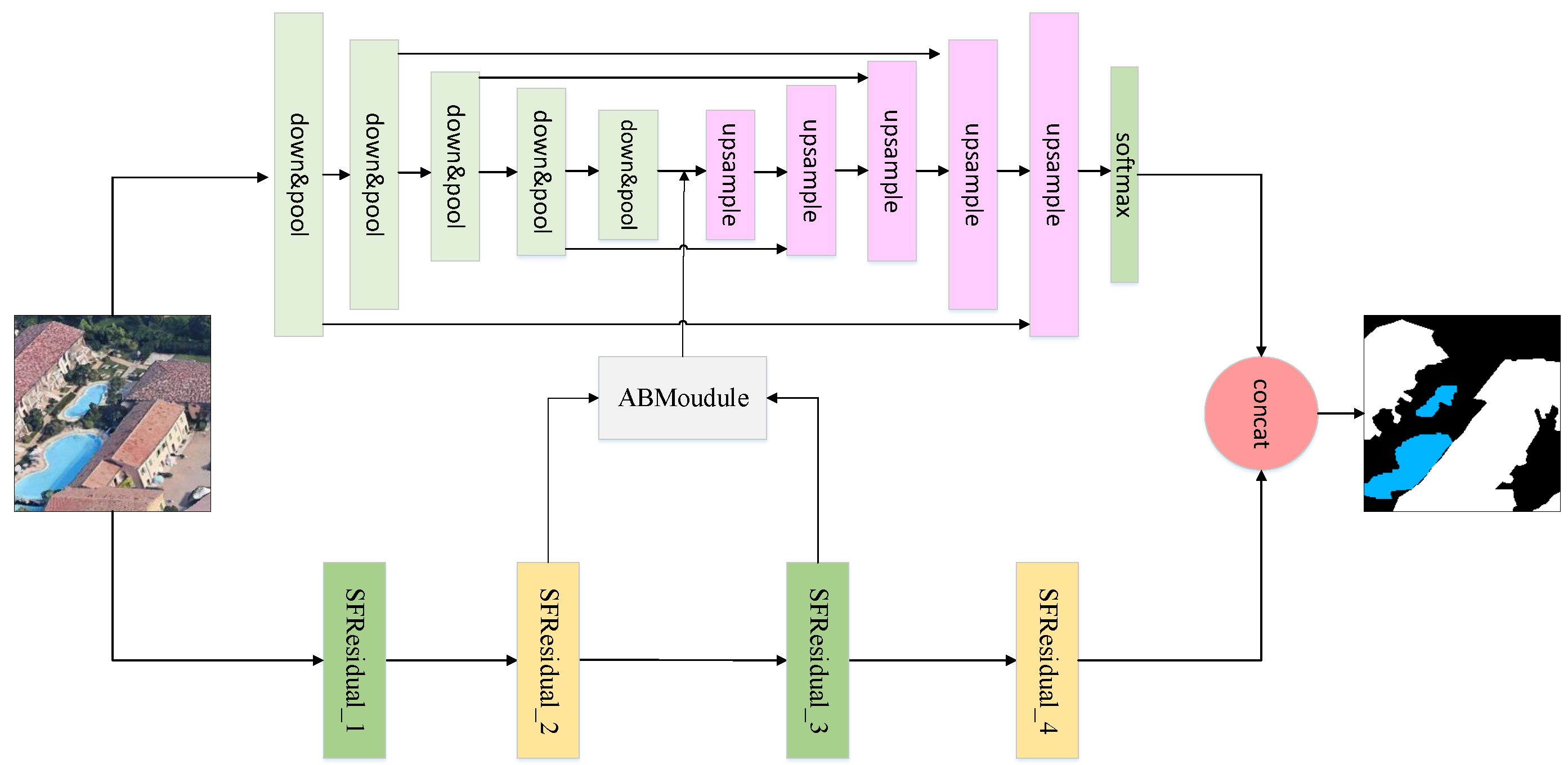
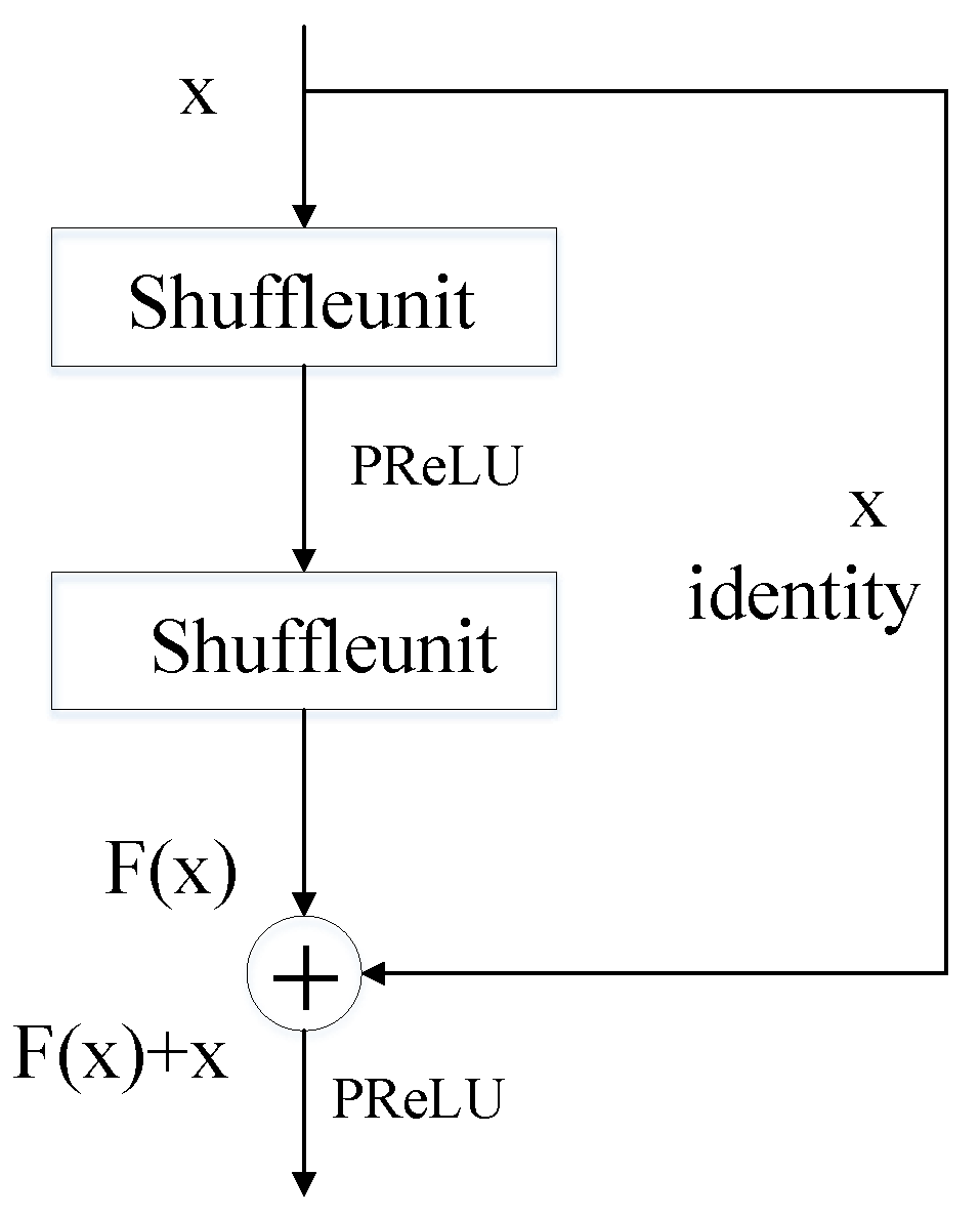
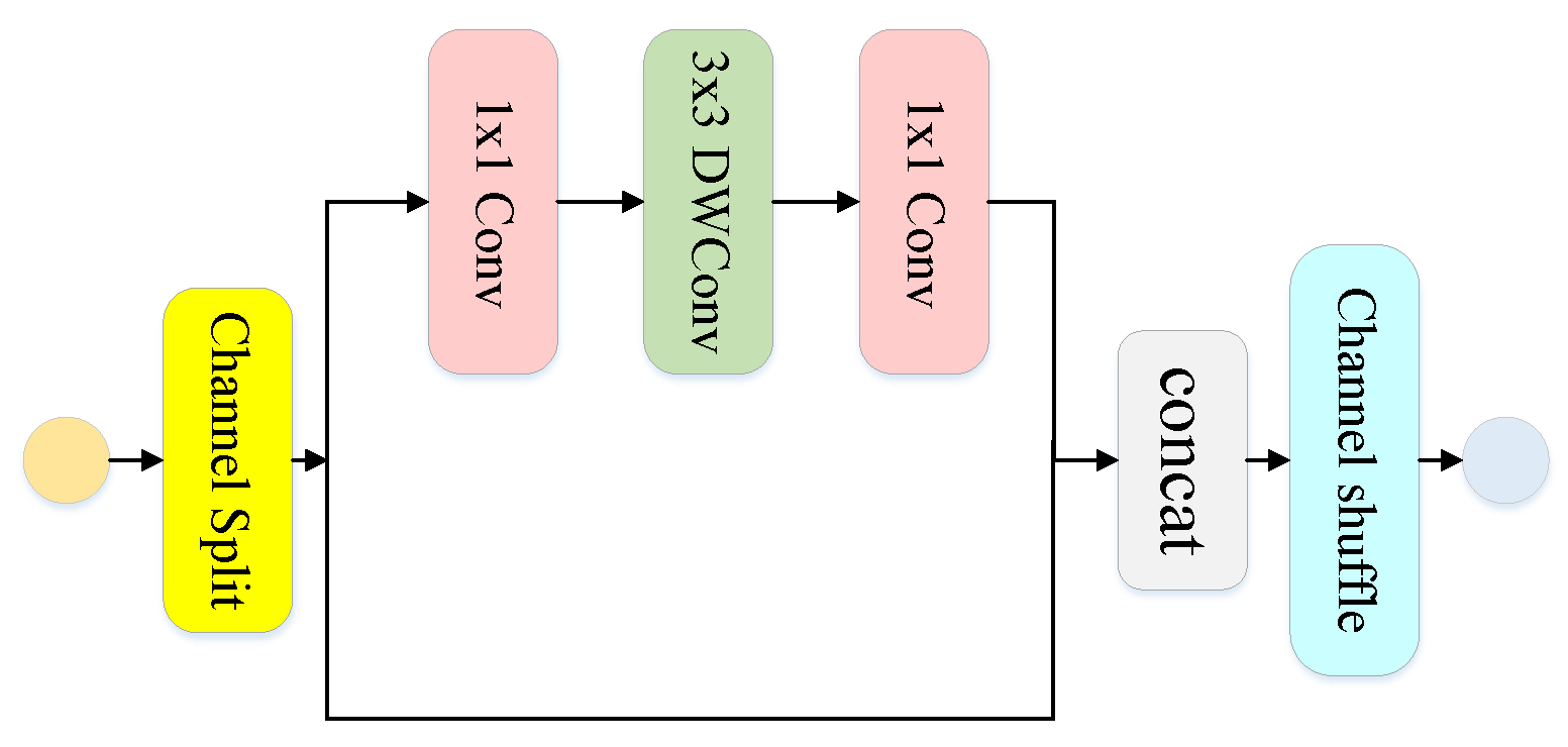
Table 2, the main module used the SHResidual module as the backbone network, and the training parameters of all models were set to the same values. According to the information in the table, the EFAModule was improved by 1.03% because of the module’s ability to recover detailed information and capture boundary information. The branch composed of the DCModule and EFAModule improved by 4.03%. The GDC_branch, which was connected with the DCModule and EFAModule, was able to greatly improve the segmentation effect. This combination paid attention to contextual information, detail features, and boundary information at the same time, which improved the accuracy of the final MSNet by 5.71% (learning rate = 0.001, power = 0.9, weight decay rate = 0.0001, batch = 4, epoch = 300).
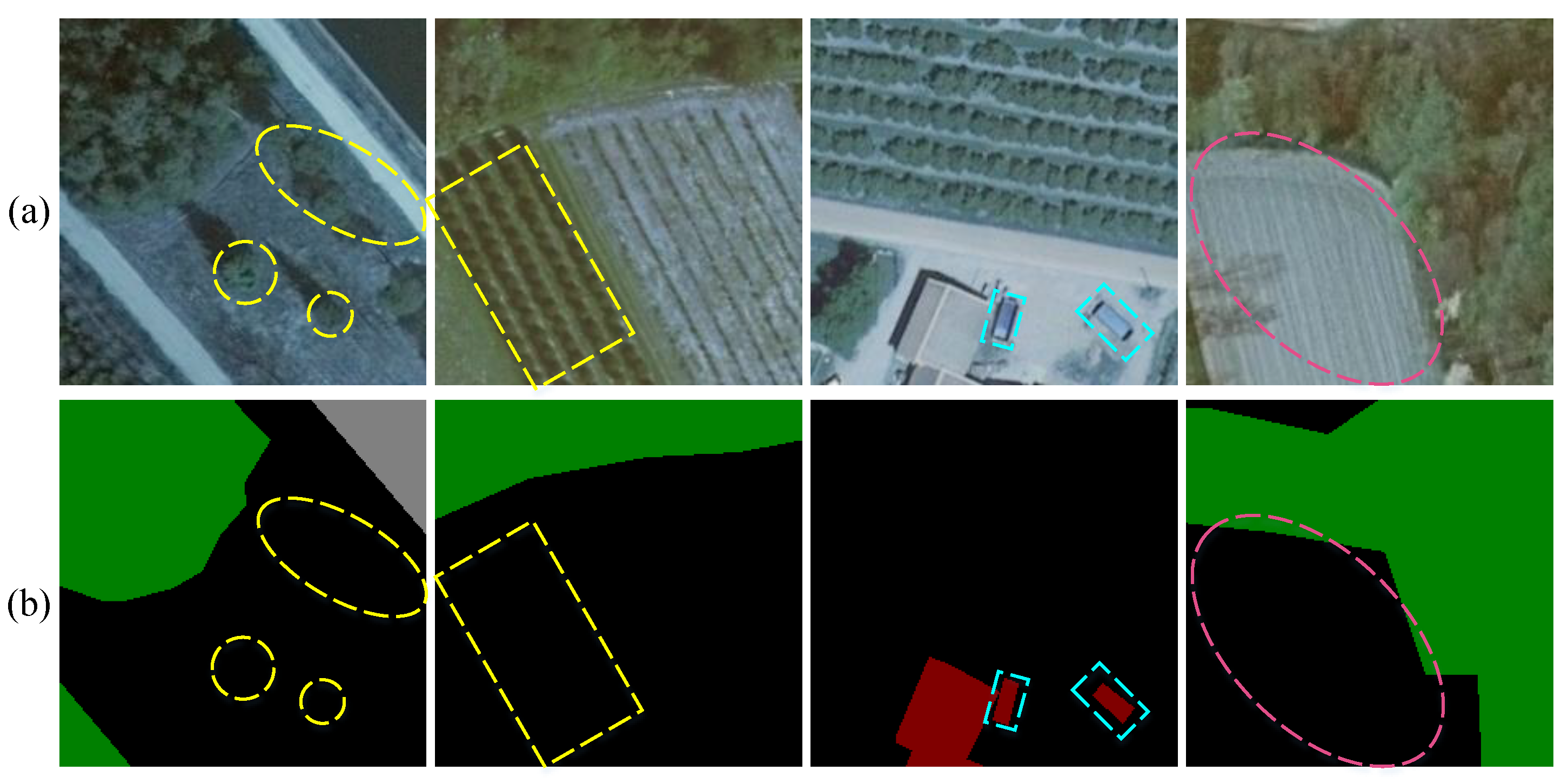
The maps that included the EFAModule obviously avoided many misclassifications and achieved a better edge segmentation effect, which was beneficial in that it was possible to extract logical features and output high-resolution detailed information. In comparison with the SFRModule alone, the combination did not misdetect the underground with respect to the buildings. Obviously, the combination of SFR, LIU, and the EFA basically allowed all of the misclassifications and edge blur to be avoided, which largely improved the segmentation effect. A diagram of the effects in the ablation experiment is shown in
Figure 10.
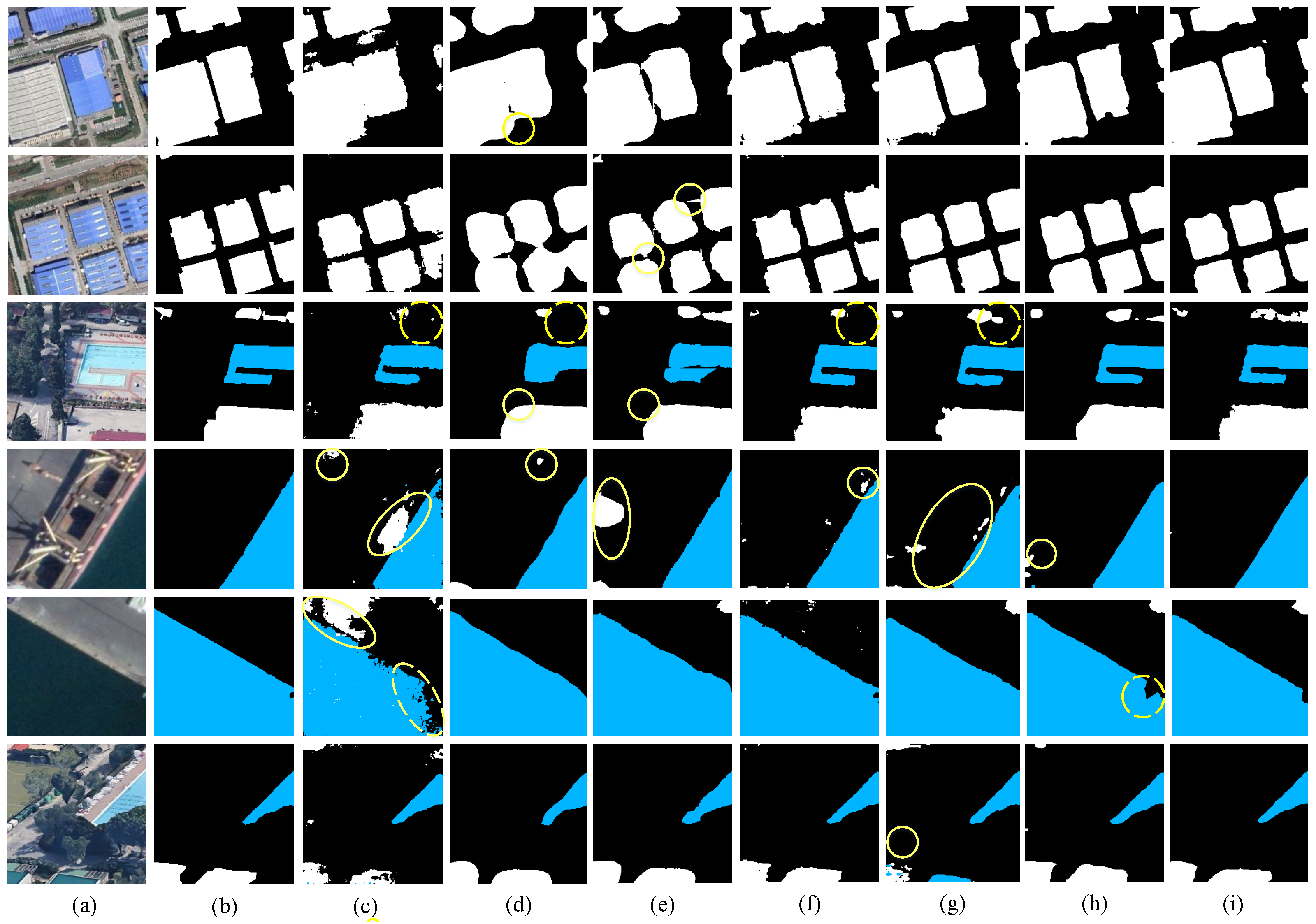
To compare the performance of each model, the models were tested under the same conditions.
Figure 11 shows a chart comparing the effects of MSNet and the other models. In the first and second sets of images, under the influence of vehicles, lawns, and other objects, networks such as FCN and SegNet showed different degrees of misdetection. SegNet mistakenly recognized the background as the buildings. The problem of edge blurring in images assessed with ExtremeC3Net was obvious, but our model achieved accurate segmentation. In the third set of images, the low buildings above the swimming pool were easily recognized as the background, though networks such as SegNet and PSPNet had obvious omissions in their recognition of buildings. In the fourth and fifth groups of images, although there was interference from the boat and the cement on the land by the sea, our model still achieved a more accurate segmentation of the water, whereas the other models misclassified the boat and the cement on the land as buildings, especially SegNet and ExtremeC3Net. In fact, the boat and the cement on the land should have been classified as background. In the sixth set of images, the blue buildings were easy to recognize as water, as they were by ExtremeC3Net, but our model still avoided such mistakes. This was caused by the synchronous learning of intra-class information and inter-class information by the SFRModule; by combining it with the EFAModule, the high-frequency detailed information was restored and the accuracy of the edge segmentation was ensured. Finally, the fusion with LIU caused our model to achieve a great effect. As shown in
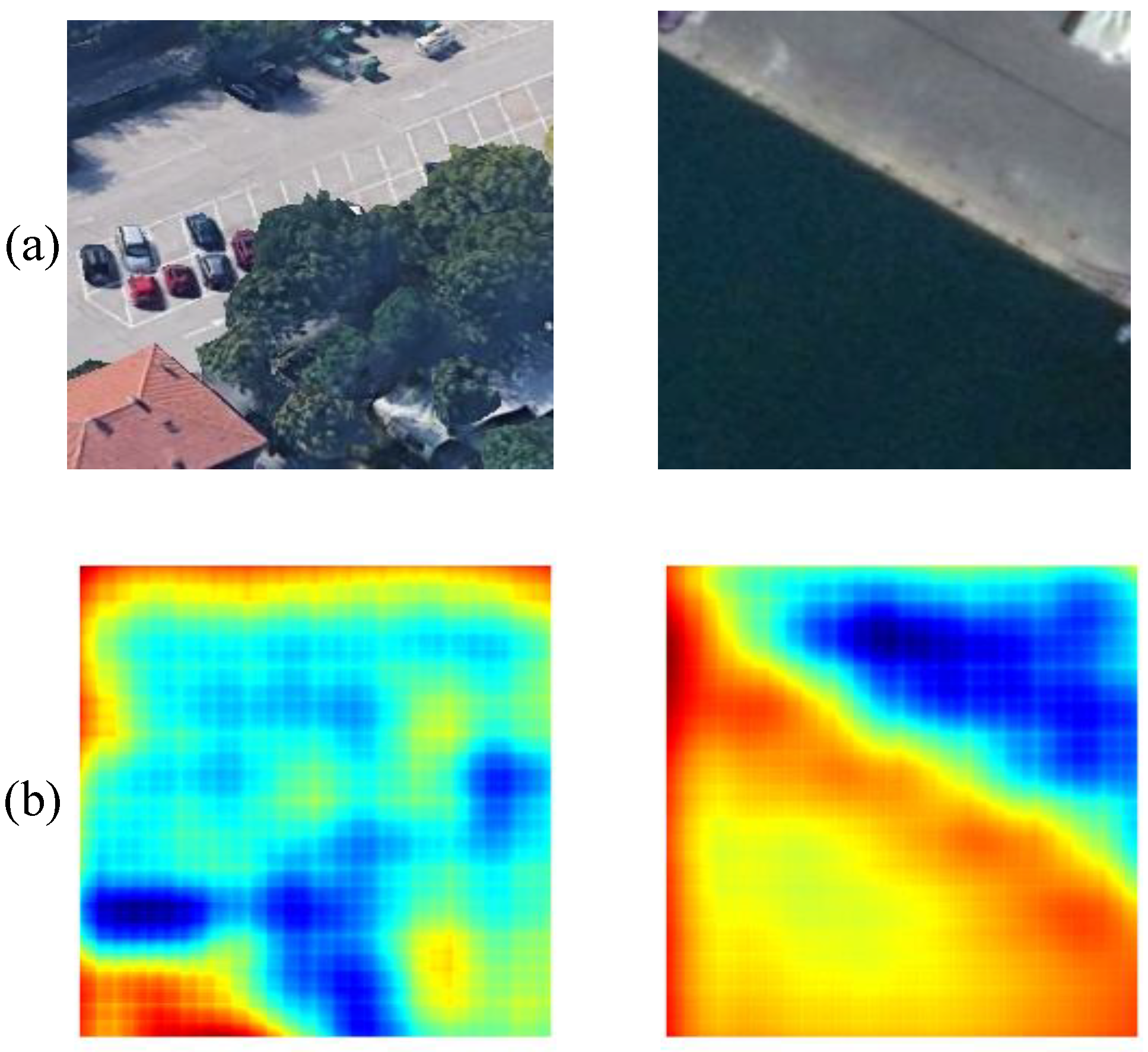
Figure 11, the actual segmentation effect of MSNet was better than that of the other networks (learning rate = 0.001, power = 0.9, weight decay rate = 0.0001, batch = 4, epoch = 300) And the heat map of this data set is shown as
Figure 12.
Table 3 shows the evaluation metrics of each model, and the PA represents the pixel accuracy of each category in the three categories. In comparison with FCN-32s, SegNet, DABNet, UNet [
33], EspNet [
46], ShuffleNetv1 [
20], and the other models, MSNet was able to achieve the best results, which were 1.19% higher than the second best index.
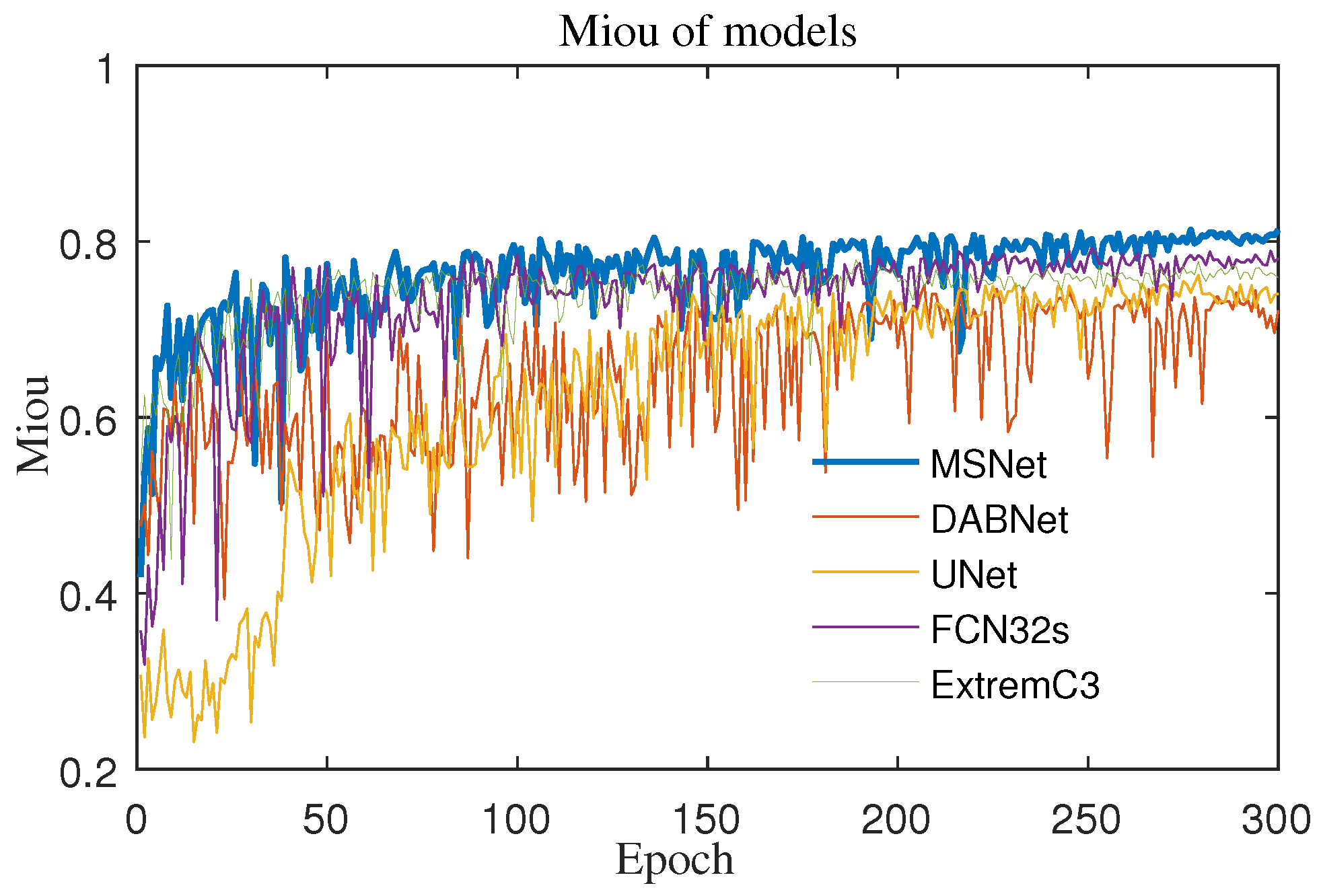
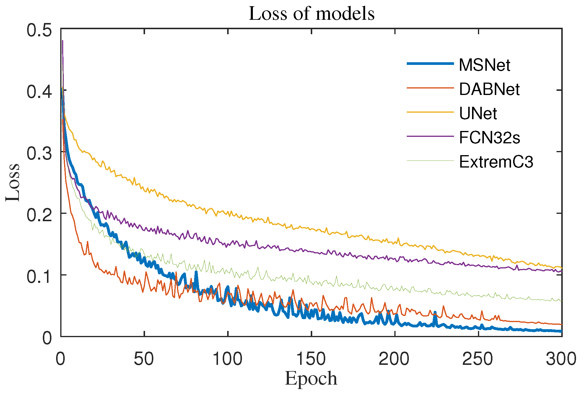
The MIoU curve of the model is shown in
Figure 13 below. In the first 50 generations of ExtremeC3Net [
52], the growth rate was very fast—better than that of MSNet (MFNet) after 100 generations—but the MSNet curve could be steadily maintained above other models. The same was true for the training loss curve (
Figure 14). In the first 50 generations, it was significantly higher than that of DABNet, and it was stable at the bottom of all curves after 100 generations. From the point of view of the convergence speed and long-term effect, MSNet had great superiority.
We provide a “feature space analysis” to show the segmentation of MSNet. In the
Figure 12, red represents the segmentation object and blue represents the background. Through the graphic analysis of the thermal diagram, it could be seen that MSNet’s segmentation of the buildings at the lower-left corner was more accurate in the first image, but the shadows at the upper-left corner were wrongly detected as buildings. For the second image, MSNet was able to accurately detect the overall scope of the water area, but the center of the water area had a false detection.
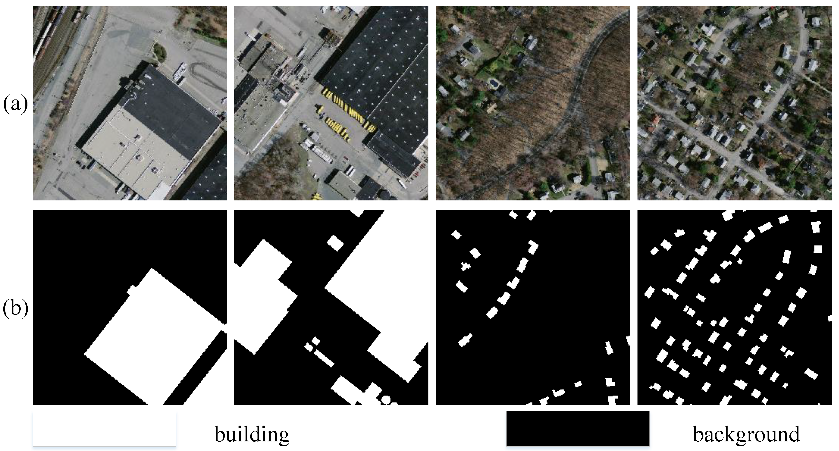
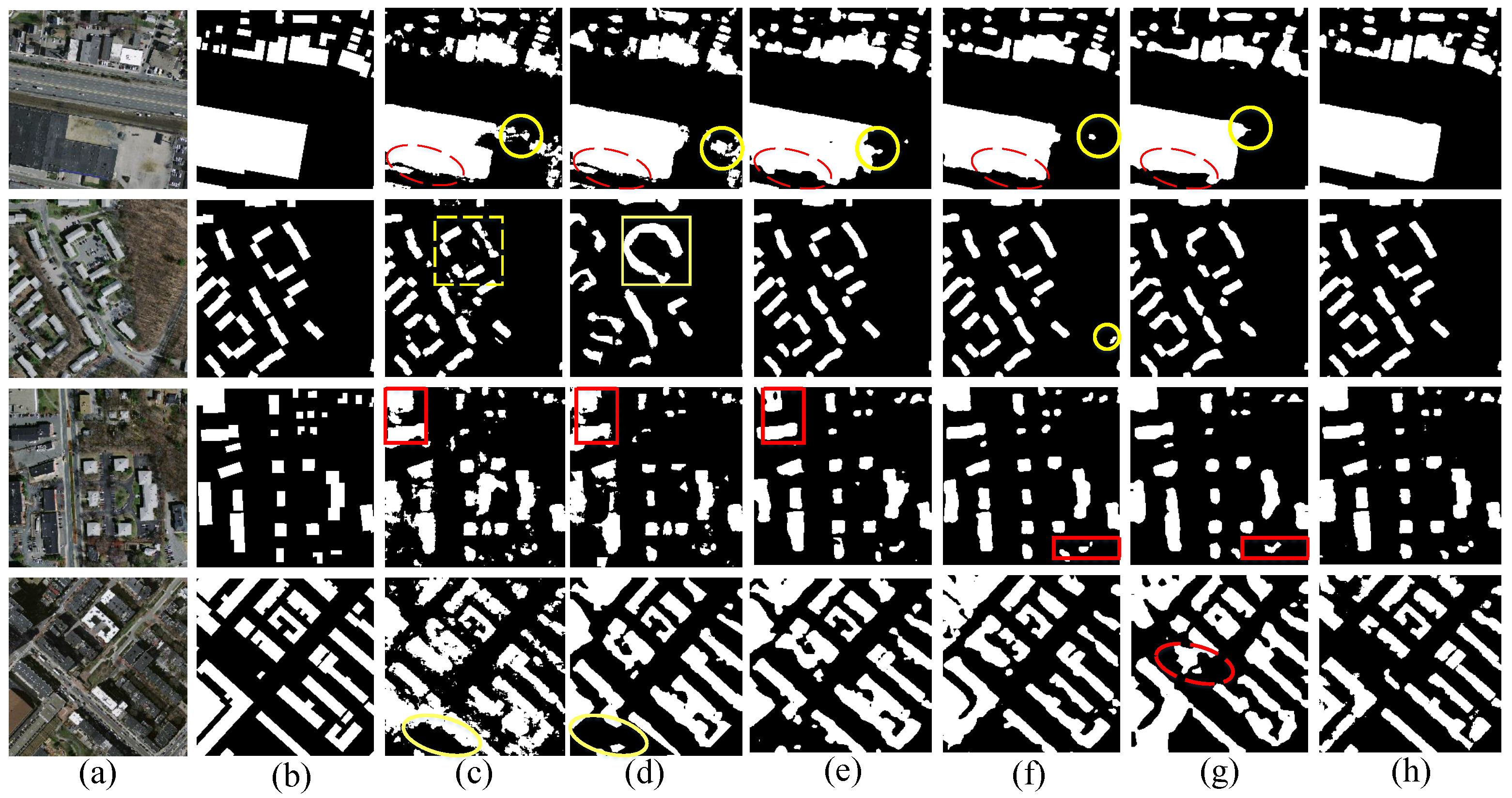
For the sake of verifying the generalization ability of the model, further experiments were carried out on the public land-cover dataset. The dataset consisted of 310 aerial images in the Boston area, each with
pixels and an area of 225 hectares. The entire dataset covered about 34,000 hectares. It was cut into 10,620 small images (
), which were divided into a training set and verification set at a ratio of 7:3 [
45]; this dataset had only the building (white, RGB [0, 0, 0]) and the background (black, RGB [255, 255, 255]) types. Without data enhancement, the settings of the various hyperparameters, except for the batch size of 3, were the same as those in the previous experiment. For the first set of images, it was obvious that MSNet’s edge segmentation effect was much better than those of FCN32s and DeepLabV3Plus. For the second, third, and fourth sets of images, the abilities of PSPNet and DABNet to segment small and dense buildings were relatively poor, but our model had accurate recognition of those buildings, including their edge information and detailed information. In terms of indicators, it was 1.01% better than the second best model and 9.44% better than the lowest model. The experimental results are shown in
Table 4 and
Figure 15 (learning rate = 0.001, power = 0.9, weight decay rates = 0.0001, batch = 4, epoch = 300).
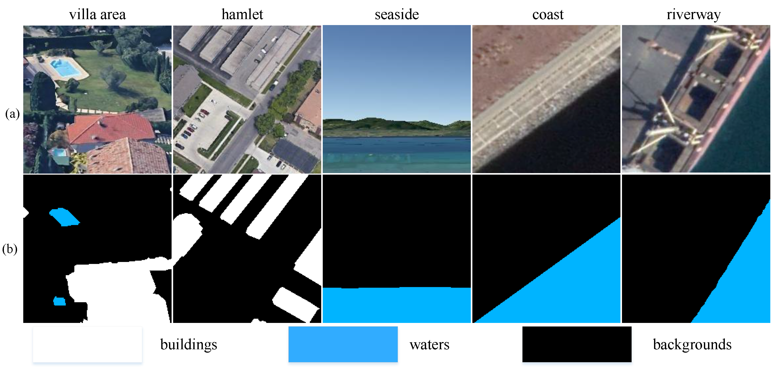
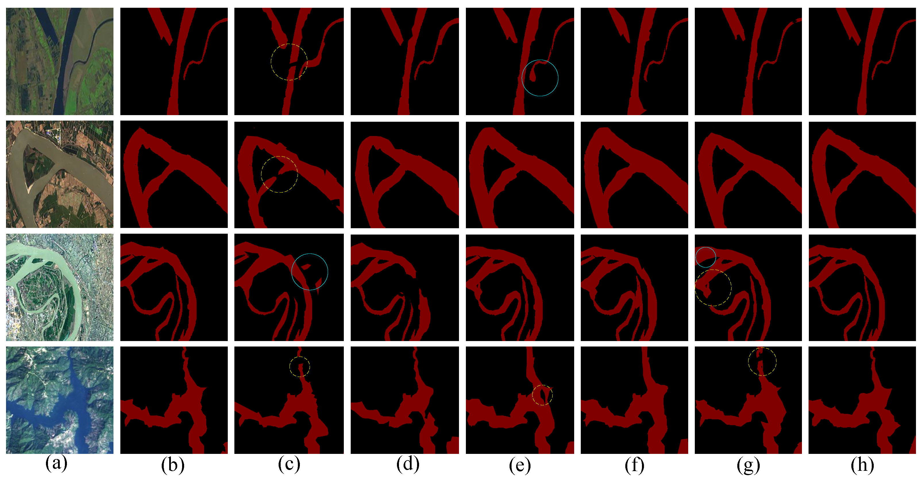
To verify the performance of the model with other categories of datasets, further experiments were carried out on a public water-cover dataset (
Figure 16). The data in this paper came from high-resolution remote sensing images selected from Google Earth, and the number of images in the data was 26,200. In order to make the data more authentic, we used a wide range of distributions, and in terms of river selection, we chose rivers with different widths and colors and small and rugged rivers. On the other hand, we selected complex environments surrounding the rivers, including hills, forests, urban areas, farmlands, and other areas, which could fully test the generalization performance of the model. Some of the images of the river that were collected are shown in
Figure 15. The average size of the Google Earth images was
pixels, and this was cut to
for model training. The training set and test set contained 20,960 and 5240 images, respectively. This dataset had only the building (red, RGB [128, 0, 0]) and the background (black, RGB [255, 255, 255]) types. Without data enhancement, the settings of the various hyperparameters, except for the batch size of 3, were the same as those in the previous experiment. For the first set of images, it was obvious that MSNet’s edge segmentation effect was much better than those of SegNet and DeepLabV3Plus. There were also obvious fractures in SegNet’s effect for the first and second sets of images. For the third and fourth groups of maps, SegNet and DABNet mistakenly detected the grassland and buildings as water areas, and DeeplabV3+ mistakenly detected an intersection of rivers as the background. The edge detection accuracy of PSPNet was relatively low, and it also mistakenly detected a water area as the background. However, MSNet could not only distinguish water areas from grasslands, buildings, and other backgrounds, but could also accurately extract edge information. In terms of indicators, it is 2.82% better than the second better model and 10.4% higher than the worst model. The experimental results are shown in
Table 5 and
Figure 15 (learning rate = 0.001, power = 0.9, weight decay rates = 0.0001, batch = 4, epoch = 300).
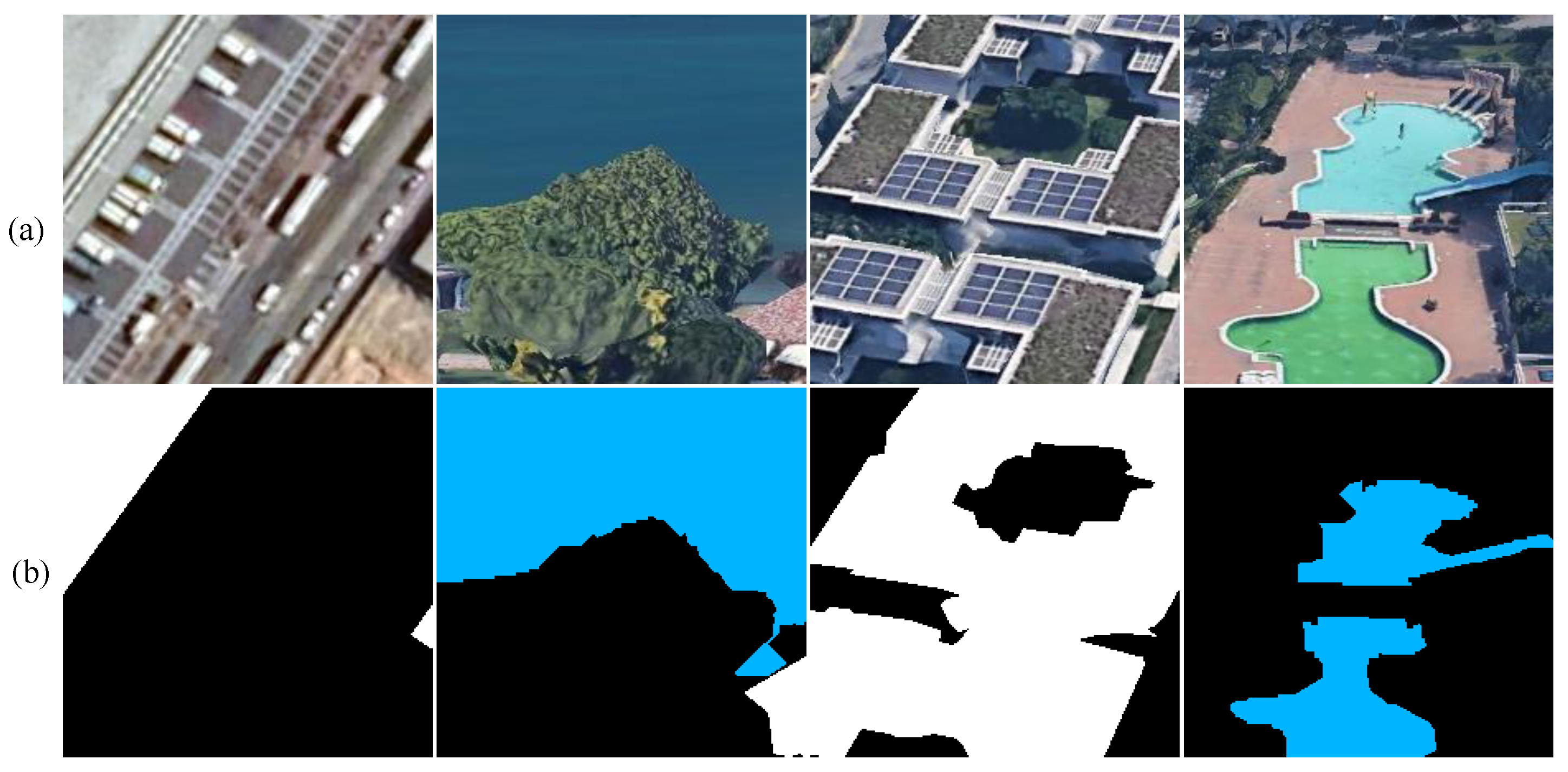
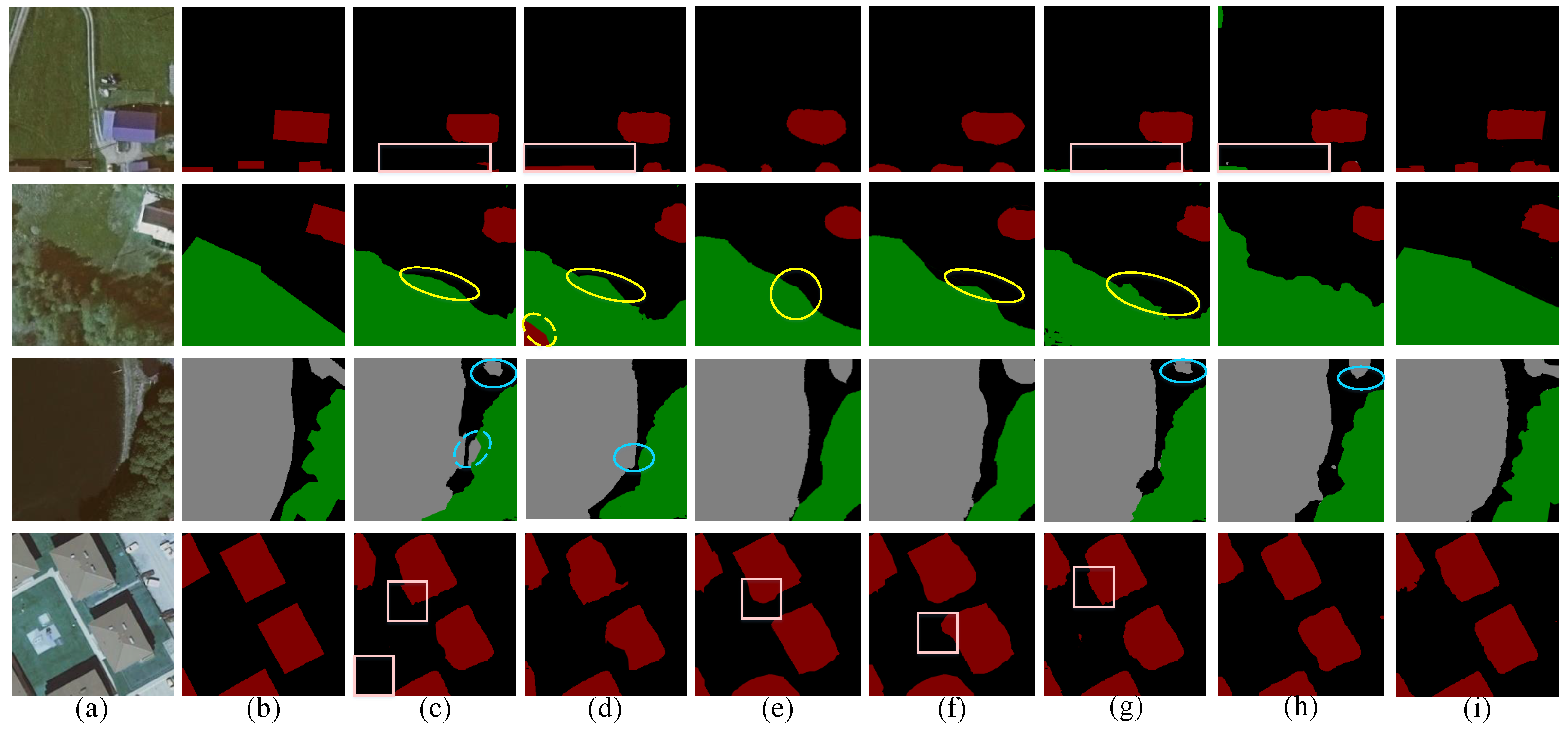
In order to include all objects in the scene, the four-class public dataset introduced above
Figure 15 was selected for a generalization experiment. As shown in
Figure 17, for the first set of images, UNet directly missed all buildings in the lower-left corner. FCN32s and DeepLabV3plus missed the detection to varying degrees. DABNet mistakenly detected buildings as plants. MSNet did not have these problems, as it benefited from SFR’s synchronous learning of intra-class information and inter-class information. For the second set of pictures, SegNet mistakenly classified the plants in the lower-left corner as buildings, and UNet, ExtremeC3Net, and the other networks mistakenly classified the background in the middle of the figure as plants. MSNet did not have this error. For the third and fourth sets of pictures, UNet confused plants with water, and the edge detection of the buildings was relatively fuzzy. The learning of the edge information of DeepLabV3plus and ExtremeC3 was not ideal, and the error was large. However, MSNet basically avoided the problems of edge blur and false recognition, which showed the superiority of the two-way fusion model. So, it can be seen intuitively that MSNet’s MIoU was higher than that of Unet by 14.3% and higher than that of FCN32s by 1.14%, as shown in
Table 6.
The results show that the average intersection ratio and the other indicators of MSNet were higher than those of the other models. Therefore, the generalization and effectiveness of MSNet were proven. MSNet combined a shuffle unit with a skip connection, the channel rearrangement caused the extraction of information to be more well distributed, and the residual structure ensured the accuracy of the extraction of deep semantic information, which paid attention to the logical relationship between information within a class and information between classes. The combination of this branch and the LIU greatly improved the accuracy of segmentation, allowed information to be extracted from a deeper level, and caused better results to be achieved. A comparison of the actual segmentation results is shown in
Figure 15, and the details of the indices are shown in
Table 6. In this experiment, the hyperparameters were set as follows: learning rate = 0.0001, power = 0.9, weight decay rate = 0.0001, batch = 4, epoch = 300.


